The Label Bias Problem
Awni Hannun January 20, 2020
Abstract
Many sequence classification models suffer from thelabel bias prob-lem. Understanding the label bias problem and when a certain model suffers from it is subtle but is essential to understand the design of models like conditional random fields and graph transformer networks.
1
Introduction
Many sequence classification models suffer from thelabel bias problem. Un-derstanding the label bias problem and when a certain model suffers from it is subtle but is essential to understand the design of models like conditional random fields and graph transformer networks.
The label bias problem mostly shows up in discriminative sequence models. At its worst, label bias can cause a model to completely ignore the current observation when predicting the next label. How and why this happens is the subject of this section. How to fix it is the subject of the next section. Suppose we have a task like predicting the parts-of-speech for each word in a sentence. For example, take the sentence “the cat sat” which consists of the tokens [the, cat, sat]. We’d like our model to output the sequence
[ARTICLE, NOUN, VERB].
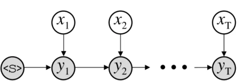
A classic discriminative sequence model for solving this problem is the maxi-mum entropy Markov model (MEMM) [McCallum et al., 2000]. The graphi-cal model for the MEMM is shown in Figure 1. Throughout,X= [x1, . . . , xT]
is the input or observation sequence and Y = [y1, . . . , yT] is the output or
x
1x
2y
1y
2<
s
>
x
Ty
TFigure 1: The graphical model for the maximum entropy Markov model (MEMM).
The MEMM makes two assumptions about the data. First,ytis
condition-ally independent of all previous observations and labels given xt and yt−1.
Second, the observations xt are independent of one another. The first
as-sumption is more central to the model while the second sometimes varies and is easier to relax. These assumptions can be seen from the graphical model. Mathematically, the model is written as
p(Y |X) =
T
Y
t=1
p(yt|xt, yt−1). (1)
The probabilities are computed with a softmax:
p(yt|xt, yt−1) =
es(yt,xt,yt−1)
Pc
i=1es(yi,xt,yt−1)
(2)
wherecis the number of output classes and s(yt, xt, yt−1) is a scoring
func-tion which should give a higher score forytwhich are likely to be the correct
label. Since we normalize over the set of possible output labels at each time step, we say the model is locally normalized and p(yt |xt, yt−1) are the
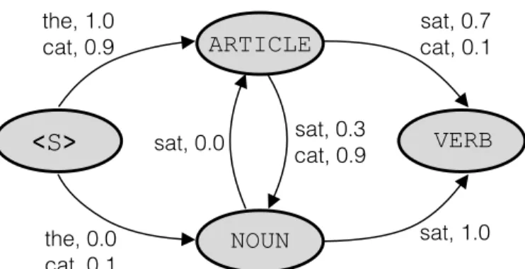
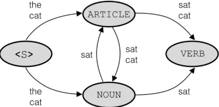
lo-cal probabilities. The distribution p(Y |X) is valid since summing over all possibleY of lengthT equals one, and all the values are non-negative. Let’s return to our example of [the, cat, sat]. We can represent the inference process on this sequence using a graph, as in Figure 2. The states (or nodes) represent the set of possible labels. The transitions (or edges) represent the possible observations along with the associated probabilities p(yt | xt, yt−1).
To compute the probability of [ARTICLE, NOUN, VERB], we just follow the observations along each arc leading to the corresponding label. In this case the probability would be 1.0×0.9×1.0.
<S>
VERB ARTICLE NOUN the, 1.0 cat, 0.9 sat, 0.7 cat, 0.1 sat, 0.3 cat, 0.9 sat, 0.0 sat, 1.0 the, 0.0 cat, 0.1Figure 2: An inference graph for the MEMM with the label set{ARTICLE, NOUN, VERB}. Each arc is labelled with the probability of transitioning to the correspond-ing state given the observation. The sum of the probabilities on arcs leavcorrespond-ing a node for a given observation should sum to one. For simplicity not all observation, score pairs are pictured.
As another example, say we drop the article and just have the sequence
[cat sat]. While it’s not a great sentence, the correct label should be
[NOUN, VERB]. However, if we follow the probabilities we see that the score for[ARTICLE, NOUN]is 0.9×0.3 = 0.27 whereas the score for [NOUN, VERB]
is 0.1×1.0 = 0.1.
The model is not used to seeing cat at the start of a sentence, so the scores leading from the start state are poorly calibrated. What we need is information about how uncertain the model is for a given observation and previous label pair. If the model has rarely seen the observation catfrom the starting node<S>then we want to know that, and it should be included in the scores.
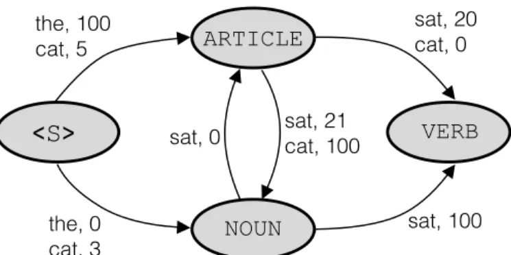
It’s actually possible that the model did at some point implicitly store this uncertainty information. However, by normalizing the outgoing scores for a given observation, we are forcing this information to be discarded. Take a look at theunnormalized inference graph in Figure 3.
The unnormalized inference graph corresponds exactly to the normalized in-ference graph when the scores are exponentiated and normalized. However, we see something interesting here. The outgoing scores for cat from <S>
are small. Recall lower scores are worse. This means the model is much less confident about the observationcat from the start state than the observa-tion the which has a score of 100. This information is completely erased when we normalize. That’s one symptom of the label bias problem.
<S>
VERB ARTICLE NOUN sat, 0 the, 100 cat, 5 sat, 20 cat, 0 sat, 21 cat, 100 sat, 100 the, 0 cat, 3Figure 3: An unnormalized inference graph for the MEMM with the label set
{ARTICLE, NOUN, VERB}. Each arc is labelled with the score of transitioning to the corresponding state given the observation. For simplicity not all observation, score pairs are pictured.
Notice in the unnormalized graph, the score for[ARTICLE, NOUN]is 5+21 = 26 while the score for [NOUN, VERB] is 3 + 100 = 103. The right answer gets a better score in the unnormalized graph! Note, we are adding scores here instead of multiplying them because the unnormalized scores are in log-space. In other wordsp(yt|xt, yt−1)∝es(yt,xt,yt−1).
We can see the label bias problem quantitatively. This observation is due to Denker and Burges [1994]. Suppose our scoring function s(yt, xt, yt−1)
factorizes into the sum of two functionsf(yt, xt, yt−1) andg(xt, yt−1).
Sup-pose further that f(·) mostly cares about how good the predicted label yt
is given the observation xt, whereas g(·) mostly cares about how good the
observation xt is given the previous label yt−1. If we compute the local
probabilities using this factorization, we get: p(yt|xt, yt−1) = ef(yt,xt,yt−1)+g(xt,yt−1) Pc i=1ef(yi,xt,yt−1)+g(xt,yt−1) = e f(yt,xt,yt−1) Pc i=1ef(yi,xt,yt−1) . (3)
The contribution of g(·) in the numerator and denominator cancels. This causes all the information about how likely the observation is given the previous state to be erased.
1.1 Conservation of Score Mass
The label bias problem results from a “conservation of score mass” [Bot-tou, 1991]. Conservation of score mass just says that the outgoing scores
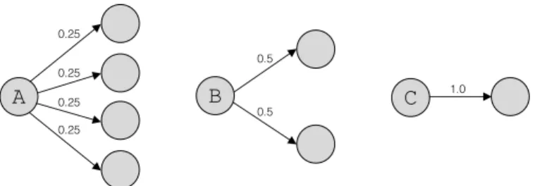
A 0.25 0.25 0.25 0.25 B 0.5 0.5 C 1.0
Figure 4: An example of three states, A,B and C, which have uniform outgoing transition distributions. Label bias will cause the inference procedure to favor paths which go through stateC.
from a state for a given observation are normalized. This means that all of the incoming probability to a state must leave that state. An observation can only dictate how much of the incoming probability to send where. It cannot change the total amount of probability leaving the state. The net result is any inference procedure will bias towards states with fewer outgoing transitions.
Suppose we have three states, A, B and C, shown in Figure 4. State A has four outgoing (nonzero) transitions, state B only has two and state C has just one. Suppose all three states distribute probability mass equally among their successor states: p(yt|xt, yt−1) is uniform.
Neither state A, B nor C are doing anything useful here, so we shouldn’t prefer one over the other. But the inference procedure will bias towards paths which go through stateCoverBand A. Paths which go through Awill be the least preferred. To understand this, suppose that the same amount of probability arrives at the three states. StateAwill decrease the probability mass for any path by a factor of four, whereas state B will only decrease a given path’s score by a factor of two and stateCwon’t penalize any path at all. In every case the observation is ignored, but the state with the fewest outgoing transitions is preferred.
Even if outgoing transitions from statesAand Bdid not ignore their obser-vations, they would still reduce a paths score since the probabilities aren’t likely to be one. This would cause state C to be preferred even though it always ignores it’s observation.
a, 0.5 b, 0.5 a, 0.5 b, 0.5 B (b) a, 0.9 b, 0.1 a, 0.1 b, 0.9 C (c) a, 0.9 b, 0.9 a, 0.1 b, 0.1 A (a)
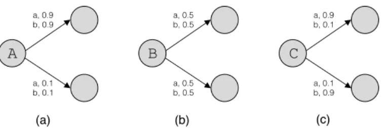
Figure 5: An example of three states,A,BandC, each with two possible outgoing transitions. Each transition is labelled with the observation and probability pair for two observations,aandb.
1.2 Entropy Bias
In a less contrived setting where the distribution p(yt | xt, yt−1) is not the
same for every observation, our model will bias towards states which have a low entropy distribution over next states given the previous state. Note this is distinct from the distribution p(yt|xt, yt−1) which can have low entropy
without directly causing label bias. However, if the conditional distribution p(yt|yt−1) has low entropy then we are potentially in trouble. For example,
in the figure above,p(y|B) has lower entropy thanp(y|A).
Consider the three in Figure 5. In each case there are two possible ob-servations a and b and two possible successor states. We’d like to know which one will introduce the most label bias into the model. To answer that question, we need to make an assumption about the prior proba-bility over observations. Suppose that the prior, p(xt), is uniform (e.g.
p(a) =p(b) = 0.5).
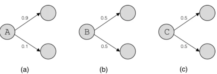
We can calculatep(yt|yt−1) for any state since
p(yt|yt−1) = X i p(yt|xi, yt−1)p(xi) = 1 n X i p(yt|xi, yt−1) (4)
where we used the fact thatp(xt) is uniform and there arenpossible
obser-vations. In our casen = 2. Figure 6 showsp(yt|yt−1) on the corresponding
arc for each example.
Case (a) has the lowest entropy transition distribution whereas case (b) and (c) are equivalent. Intuitively, we expect case (a) to be worse than case (b) since it biases towards the upper path, whereas (b) does not bias towards either. However, case (c) is interesting. In case (c), the observation can
0.5 0.5 B (b) 0.5 0.5 C (c) 0.9 0.1 A (a)
Figure 6: An example of three states,A,BandC, each with two possible outgoing transitions. Each transition is labelled with the probabilityp(yt|yt−1) which are
computed from the probabilities in the figure above.
have a large effect on the outcome. While this effect might be wrong if the probabilities are poorly calibrated, this case doesn’t cause label bias more than case (b) under the assumption of a uniform prior.
1.3 Revising Past Mistakes
Another description of the label bias problem is that it does not allow a model to easily recover from past mistakes. This follows from the conser-vation of score mass perspective. If the outgoing score mass of a path is conserved, then at each transition the mass can only decrease. In the fu-ture, if a path encounters new evidence which makes it very likely to be correct, it cannot increase the path’s score. The most this new evidence can do is to not decrease the path’s score by preserving all of the incoming mass for that path. So the model’s ability to promote a path given new evidence is limited even if we are certain that the new observation makes this path the correct one.
2
Overcoming the Label Bias Problem
As we observed in the [cat, sat] example above, if we don’t normalize scores at each step, then the path scores can retain useful information. This implies that we should avoid locally normalizing probabilities.
One option is that we don’t normalize at all. Instead, when training, we simply tune the model parameters to increase the score
s(X, Y) =
T
X
t=1
s(yt, xt, yt−1) (5)
for every (X, Y) pair in our training set. The problem with this is there is no competition between possible outputs. This can result in the model maximizing s(Y, X) while completely ignoring its inputs. So we need some kind of competition between outputs. If the score of one output goes up, then others should feel pressure to go down.
This can be achieved withglobal normalization. We compute the probability as p(Y |X) = e PT t=1s(yt,xt,yt−1) P Y0∈Y Te PT t=1s(y 0 t,xt,y 0 t−1) (6) where YT is the set of all possible Y of length T. This is exactly a linear chain conditional random field (CRF) [Lafferty et al., 2001]. The graphical model and hence dependency structure is the same as the MEMM in the previous section. The only difference is how we normalize the scores for a given input.
With this normalization scheme, the label bias problem is no longer an issue. In fact when performing inference, we need not normalize at all. The nor-malization term is constant for a givenXand hence the ordering between the possibleY will be preserved without normalizing. What this means is that the inference procedure operates on an unnormalized graph just like the one we saw for the part-of-speech tagging example in the previous section. Because transitions have unnormalized scores, they are free to affect the overall path score anyway they please. If cat is very unlikely to follow
<s> the model can retain that information by keeping the scores for all transitions out of <s> low. Then whenever we see cat following the state
<s>, the path score won’t be affected much since the model is uncertain of what the correct next label is.
This freedom from the label bias problem comes at a cost. Computing the normalization term exactly is more expensive with a CRF than with an MEMM. With an MEMM we normalize locally. Each local normalization costsO(c) where c is the number of classes, and we have to compute T of them, so the total cost is O(cT). With a linear chain CRF, on the other-hand, the total cost using an efficient dynamic programming algorithm called the forward-backward algorithm, isO(c2T) [Sutton et al., 2012]. Ifcis large
this can be a major hit to training time. For more complex structures where there can be longer-range dependencies between the outputs, beam search is usually the only option to approximate the normalization term [Collobert et al., 2019].
3
A Brief History of the Label Bias Problem
The first recorded observation of the label bias problem was by Bottou [1991]. The term “label bias” was coined in the seminal work of Lafferty et al. [2001] introducing conditional random fields. Solving the label bias problem was one of the motivations for developing the CRF. The CRF was one of earliest discriminative sequence models to give a principled solution to the label bias problem.An even earlier sequence model which overcame the label bias problem was the check reading system proposed by Denker and Burges [1994], though they did not use the term label bias. This work motivated the graph transformer networks of Bottou et al. [1997]. More references on graph transformer networks can be found on L´eon Bottou’s webpage on structure learning systems1.
4
A Few Examples
In this section we’ll look at a few examples of models, some of which suffer from label bias and some of which do not.
4.1 Hidden Markov Model
The hidden Markov model (HMM) is a generative model which makes two assumptions about the data generating distribution. First, it assumes that the observationxtis conditionally independent of all otheryandxgiven the
hidden state (i.e. label) at time t, yt. Second, the HMM makes the usual
Markov independence assumption thatytis conditionally independent of all
previousy given yt−1. In equations
x
1x
2y
1y
2<
s
>
x
Ty
TFigure 7: The graphical model for the hidden Markov model (HMM).
<
S
>
VERB ARTICLE NOUN the cat sat cat sat cat sat sat the catFigure 8: An inference graph for the HMM with the label set{ARTICLE, NOUN, VERB}. The scores for the given observation on each arc are not shown.
p(X, Y) =p(y0)
T
Y
t=1
p(xt|yt)p(yt|yt−1). (7)
This is a very different model from the MEMM. It’s generative, not dis-criminative, so we estimate p(X, Y) and not p(Y | X). Interestingly, the only difference between the graphical model for an HMM (Figure 7) and the MEMM is the direction of the arrows between xt and yt.
As a simple rule of thumb, generative models do not suffer from label bias. One way to see this for the HMM specifically is to look at the corresponding inference graph, as in Figure 8.
The scores on each edge associated with an observation are given by p(xt|
yt)p(yt | yt−1). In general the sum of these scores over all possible next
states is not required to be one:
c
X
i=1
More importantly, the sum is not a constant, but can change depending on the observation and the previous state. This implies that we do not have conservation of score mass and hence label bias is not an issue.
4.2 Sequence-to-sequence Models
Sequence-to-sequence models with attention are very commonly used to la-bel sequences. These models are discriminative and compute the probability of an output given an input using the chain rule
p(Y |X) =
T
Y
t=1
p(yt|y<t, X) where p(yt|y<t, X)∝es(yt,y<t,X). (9)
The score functions(·) is computed using a multi-layer neural network with attention.
These models are locally normalized,
c
X
i=1
p(yi|y<t, X) = 1, (10)
hence they can suffer from label bias. Whether or not this is an issue in practice remains to be seen. Some attempts have been made to design globally normalized versions of these models, though none are yet commonly used [Wiseman and Rush, 2016].
4.3 Connectionist Temporal Classification
Connectionist Temporal Classification (CTC) is a discriminative sequence model designed to solve problems where the correspondence between the input and output sequence is unknown [Graves et al., 2006] This includes problems like speech and handwriting recognition among others. See Han-nun [2017] for an in-depth tutorial.
For a given input-output pair (X, Y), CTC allows a set of alignmentsAX,Y. We letA= [a1, . . . , aT]∈ AX,Y be one such alignment. Note,Ahas the same
length asX, namelyT. The probability of a sequence Y given an input X can then be computed as
p(Y |X) = X A∈AX,Y T Y t=1 p(at|X) where p(at|X)∝es(at,X). (11)
Like sequence-to-sequence models with attention, the score function s(·) is usually computed with a multi-layer neural network. Notice that CTC assumes the outputsat are conditionally independent of one another given
the input X.
The CTC model is a special case in that it is both locally normalized and globally normalized. Because of the conditional independence assump-tion, the two are equivalent. At the level of an individual alignment, we have p(A|X) = T Y t=1 est(at,X) Pc i=1est(ai,X) = QT t=1est(at,X) QT t=1 Pc i=1est(ai,X) . (12)
We can rewrite the denominator using the fact that
m Y j=1 n X ij=1 aij = n X i1=1 ai1 . . . n X im=1 aim = m X i1=1 . . . n X im=1 m Y j=1 aij (13) to get p(A|X) = e PT t=1st(at,X) P A0e PT t=1st(a 0 t,X) . (14)
Used on its own, CTC does not suffer from label bias. There are a couple of ways to see this. First, as we described, CTC is globally normalized at the level of an alignment and label bias results from local normalization. Second, the conditional independence assumption made by CTC removes label bias. If the next state prediction does not depend on any previous state, then there is no label bias. The model acts as if the transition probabilities p(yt|yt−1) are uniform and the same for allyt−1. This means the entropies
of these distributions are all the same and maximal.
The model does have conservation of score mass in the sense thatPc
i=1p(yi|
a given path. The model can favor paths which have a certain label at a given time step by giving the corresponding p(yt|X) a value close to one.
This will in turn make all paths which do not predict yt have scores very
close to zero. However, the expressiveness of the model is also limited since it cannot select for paths based on previously predicted labels.
References
L´eon Bottou. Une Approche Th´eorique de l’Apprentissage Connexionniste: Applications `a la Reconnaissance de la Parole. PhD thesis, 1991.
L´eon Bottou, Yoshua Bengio, and Yann Le Cun. Global training of docu-ment processing systems using graph transformer networks. InProceedings of IEEE Computer Society Conference on Computer Vision and Pattern Recognition, pages 489–494. IEEE, 1997.
Ronan Collobert, Awni Hannun, and Gabriel Synnaeve. A fully differen-tiable beam search decoder. 2019.
John S Denker and Christopher CJ Burges. Image segmentation and recog-nition. In Santa Fe Institute Studies in the Sciences of Complexity, vol-ume 20, pages 409–409. Addison-Wesley Publishing Co, 1994.
Alex Graves, Santiago Fern´andez, Faustino Gomez, and J¨urgen Schmid-huber. Connectionist temporal classification: labelling unsegmented se-quence data with recurrent neural networks. In Proceedings of the 23rd international conference on Machine learning, pages 369–376. ACM, 2006. Awni Hannun. Sequence modeling with ctc.Distill, 2017. doi:
10.23915/dis-till.00008. https://distill.pub/2017/ctc.
John Lafferty, Andrew McCallum, and Fernando CN Pereira. Conditional random fields: Probabilistic models for segmenting and labeling sequence data. 2001.
Andrew McCallum, Dayne Freitag, and Fernando CN Pereira. Maximum entropy markov models for information extraction and segmentation. In
International conference on machine learning, pages 591–598, 2000. Charles Sutton, Andrew McCallum, et al. An introduction to conditional
random fields. Foundations and TrendsR in Machine Learning, 4(4):267–
Sam Wiseman and Alexander M Rush. Sequence-to-sequence learning as beam-search optimization. arXiv preprint arXiv:1606.02960, 2016.