8
CLASSIFICATION OF ACUTE LEUKEMIA
BASED ON DNA MICROARRAY GENE
EXPRESSIONS USING PARTIAL LEAST
SQUARES
Danh V. Nguyen1 and David M. Rocke1,2
1Center for Image Processing and Integrated Computing and 2Department of Applied Science,
University of California, Davis, CA 95616
Abstract: Analysis of microarray data, when presented with raw gene expression intensity data, often take two main steps when analyzing the data. First pre-process the data by rescaling and standardizing so that overall intensities for each array are equivalent. Second, apply statistical methodologies to answer scientific questions of interest. In this paper, for the data pre-processing step, we introduce a thresholding algorithm for rescaling each array. Step 2 involves statistical classification and dimension reduction methodologies. For this we introduce the method of partial least squares (PLS) and apply it to the leukemia microarray data set of Golub et al. (1999). We also discuss the use of principal components analysis (PCA), quadratic discriminant analysis (QDA) and logistic discrimination (LD). Finally, we discuss other potential applications of PLS in analyzing gene expression data that address prediction of a target gene, prediction of the reaction in cell lines, assessment of patient survival, and generalisations in predicting multiple classes.
Key words: Dimension reduction, Logistic Discrimination, Prediction, Quadratic discriminant analysis
INTRODUCTION
DNA microarray technology has revolutionised biological and medicinal research. The use of DNA microarrays allows simultaneous monitoring of the expressions of thousands of genes. In a short period of time researchers have gathered a wealth of gene expression data from microarrays (such as high density oligonucleotide arrays and cDNA arrays). Prediction,
classification, and clustering techniques are being used for analysis and interpretation of the data. For instance, molecular classification of acute leukemia [Golub et al., 1999], cluster analysis of tumor and normal colon tissues [Alon et al., 1999], clustering and classification of human cancer cell lines [Ross et al., 2000] and diffuse large B-cell lymphoma (DLBCL) [Alizadeh et al., 2000], human mammary epithelial cells and breast cancer [Perou et al., 1999, 2000], and skin cancer melanoma [Bittner et al., 2000] are some examples. These techniques have also helped to identify previously undetected subtypes of cancer [Golub et al., 1999; Alizadeh et al., 2000; Bittner et al., 2000; Perou et al., 2000]. The problem of “prediction” may come in various forms of applications as well; the prediction of patient survival duration with germinal centre B-like DLBCL compared to those with activated B-like DLBCL (gene expression subgroups) using Kaplan-Meier survival curves [Ross et al., 2000] or the prediction of a target gene expression are examples.
Gene expression data from DNA microarrays are characterized by many measured variables (genes) on only a few observations (experiments) although both the number of experiments and genes per experiment are growing rapidly. The number of genes on a single array are usually in the thousands, so the number of variables, p, easily exceeds the number of observations N. Although the number of measured genes is large there may only be a few underlying gene components that account for much of the data variation; for instance, only a few linear combinations of a subset of genes account for nearly all of the response variation. Under similar data structure in the field of chemometrics, the method of PLS (Partial Least Square) has been found to be very useful.
PLS has been useful as a predictive modelling regression method in the field of chemometrics. A typical example, in spectroscopy, is to predict the chemical composition of a compound based on observed signals for a particular wavelength, where the number of wavelengths (variables) is much larger than the number of available samples. Examples of PLS applications in chemometrics can be found in the Journal of Chemometrics (John Wiley) and Chemometrics and Intelligent Laboratory Systems (Elsevier). For an introduction to PLS regression the reader is referred to a tutorial paper by Geladi and Kowalski (1986). The use of PLS in calibration can be found in Martens and Naes (1989). Some theoretical aspects and data-analytical properties of PLS have been studied by chemometricians and statisticians [de Jong, 1993; Frank and Friedman, 1993; Goutis, 1996; Helland, 1988; Helland and Almoy, 1994; Hoskuldsson, 1988; Lorber et al., 1997; Phatak, et al., 1992; Stone and Brooks, 1990]. An interpretation of PLS based on sequences of simple linear regression can be found in Garwaithe (1994).
The method of PLS is also useful for various prediction problems based on gene expression data. We briefly introduce the method here and give details in the section on methods. For simplicity we restrict to the case where the response variable Y is univariate. For instance, the response variable can be the expression values of a single “target” gene of interest, however, if one is interested in predicting the expression values of several genes (i.e., a “block” of genes) simultaneously PLS applies as well. Multiple linear regression (MLR) is perhaps the most popular method used to predict a response variable Y based on a set of predictor variables X1, X2,..., Xp. It is
well known that when there are more predictors than there are samples (p >
N) the MLR model will fit the data perfectly, but the model will not predict
new samples well. A common approach to deal with this problem is to first reduce the dimension of the data by constructing a few summary “components” and then use this reduced set of constructed components to predict the response Y. An example of this approach is principal components regression (PCR) [Massey, 1965; Jolliffe, 1986]. Here, principle component analysis (PCA) is used to reduce the high dimensional data to only a few gene components, which explain as much of the observed total gene expression variation as possible (subject to orthogonality and norming constraints). This is achieved without regards to the response (leukemia class) variation. Gene components constructed this way are called principal components (PCs).
In contrast to PCA, PLS components are chosen so that the sample covariance between the response and a linear combination of the p predictors is maximum. The latter criterion for PLS is more sensible since there is no a priori reason why constructed components having large predictor variation (gene expression variation) should be strongly related to the response variable (leukemia classes). Certainly a component with small predictor variance could be a better predictor of the response classes. The ability of the dimension reduction method to summarize the covariation between gene expressions and leukemia classes may yield better prediction results. We will demonstrate this contrast between PLS and PCA using the leukemia data.
This paper is organized was follows. In the Methods section we describe the thresholding algorithm for array rescaling and the details of the dimension reduction method of PLS and PCA. After rescaling and dimension reduction, we considered logistic and quadratic discrimination between the leukemia classes. Results and comparison to Golub et al. (1999) are given in the section on Results. We conclude and discuss the potential applications of PLS in gene expression analysis in the sections on Conclusions and Discussions respectively.
METHODS
A Thresholding Algorithm for Rescaling Gene Expressions
Pre-processing of gene array data is common for various reasons. The main reason is the non-uniform noises associated with array technologies observed from one array (sample) to another. Thus, array rescaling (or normalization) is important since subsequent analysis results are meaningful if the overall intensities for each array are equivalent. The use of thresholding is especially common in data pre-processing. For instance, discarding negative measurements (which occurs when a spot background intensity measurement exceeds the signal intensity) or very low signal to noise measurements. Although negative measurements (due to imperfect measurement technology) should not be used in the analysis of the genes, this information can be used to estimate the amount of noise present in each array.In this section we describe a thresholding algorithm which finds a “cutoff'” point for each array (hence, accounting for different levels of noise specific to a given arrays). Genes with expression levels below the cutoff point may be considered unreliable. Also, information from the algorithm is used to estimate the amount of noise present in a particular array. Gene expression levels are then rescaled so that overall intensities for each array are equivalent based on the estimate of the average noise for each array. The algorithm is derived from a two-component error model for gene expression arrays. Due to limited space, the reader is referred to Rocke and Durbin (2000) for details of this model.
We now describe the thresholding algorithm. Let the original gene expression values for the ith array be x1, x2,..., xp and i=1, 2, ... , N is the
number of arrays. For brevity of notation we denote the collection of expression values for array i by {xj, j=1, p}={ xi1, xi2,..., xip} and assume that
these values are sorted. The algorithm begins with an initial set, A(0), consisting of noise values (negative measurements) and low signal to noise measurements (small intensity minus background). The median of A(0), say
m0, gives an initial estimate of the amount of noise specific to the given
array. Similarly, the usual sample standard deviation of A(0), say s0, gives
an initial estimate of the dispersion of the noise measurements in the given array. Thus, expression values close to m0 have high noise relative to signal
intensity. The algorithm then updates the original noise set, A(0), by adding to this set all expression values close to m0. That is, enlarge the initial set
consisting of noise measurements by adding to it expression measurements with high noise relative to signal intensity. How close to the initial estimate of array-specific noise, m0, should a particular expression measurement be in
order for it to be included in the noise set? One can, for instance, include all expression measurements within two (or three) standard deviations (s0) of
the initial array-specific noise estimate, m0. Thus, expression values below a
cutoff threshold of u0 = m0 + c⋅s0 would be added to the initial noise set A(0),
where c is the number of standard deviation away from the median noise estimate m0. However, rather than using the usual sample standard
deviation, which is highly effected by outliers, we used a robust measure of dispersion given by s0 = MAD0 / 0.675, where MAD0=median {| xj – m0 |,
j=1, n0} is the median absolute deviation about the median. Note that for the
same reason we have also used the median, rather than the mean as a measure of location, to estimate the array-specific noise.
Thus, the updated noise set now consists of all the initial noise values in A(0) and all expression values less than the cutoff threshold of u0 = m0 +
c⋅s0. Call this enlarged noise set A(1). A revised or updated estimate of the
amount of noise present in the given array is the median of the updated noise set A(1), denoted m1. Similarly, the revised robust estimate of the dispersion
of the updated noise set is s1 = MAD1 / 0.675. The updated noise set, A(1),is
again revised (updated) to include all expression values that are determined to be high in noise relative to signal intensity, namely all expression values less than u1 = m1 + c⋅s1. This updating process continues until the noise set
A(k) no longer changes. That is, the algorithm stops when the noise set A(k)
(for the ith array) converges. Denote this set by A(ni). Thus, at convergence,
the set A(ni) consists of the smallest ni values from array i. Convergence of
the algorithm is not guaranteed and in rare instances we have observed that the algorithm fluctuates between two values. If these are not too different the midpoint can be taken, for instance.
Estimate of the mean or median array-specific noise can now be obtained by taking the sample mean or median of the set A(ni), for array i. (Any
appropriate statistics based on A(ni)may be used.) Similarly, values in A(ni)
can also be used to estimate the variation of noise within an array, hence providing a way for calculating a confidence interval for a gene expression value (when no replicated gene measurements are available). In most instances the algorithm converges in less than 15 iterations. The steps of the algorithm are given below.
Thresholding Algorithm Parameters: q and c
1. Select q% of the lowest expression values. Denote this initial set of values by A(0) = {xj,j=1, n0}.
2. Calculate the median of the initial set, m0= median{A(0)}.
3. Calculate the median of the absolute deviations about the median,
4. Calculate the cutoff point, u0 = m0 + c· s0, where s0 = MAD0/0.6745 and c
=2, 2.5, or 3 (is the number of median absolute deviation above the median).
5. Determine the new set defined by A(1) = {all xj < u0}.
6. Repeat steps 2 through 5 (for each new set A(k)) and stop when nk = nk-1
(convergence). At convergence denote the set of noise values by A(nI)
(with size nI) and the cutoff point by uI for I =1,…, N.
7. Repeat steps 1 through 6 for each array, I =1,…,N.
As mentioned earlier, one application of the thresholding algorithm is to use the information from the algorithm to rescale the expression levels in each array so that overall intensities are equivalent across all arrays. We now describe this application. Suppose that the mean of A(ni), m(i) = ni-1 j xij (i=1, …, N; j=1, …, ni) is used to estimate the average noise from array i.
One may consider a (1) multiplicative rescaling: xij xij ai or a (2)
subtractive rescaling: xij xij - bi, where ai = M(i)/m(i), bi = m(i) and M(i) is
the overall mean of the ith array. Using strategy (1) to rescale an array with high average noise would result in smaller (rescaled) expression values relative to expression values of another array with lower average noise (and similar overall average expression). Even baseline or control arrays are susceptible to errors since measurements come from the same system; hence, the algorithm can be applied there as well. We have suggested only two obvious strategies for rescaling the gene expression values and we focus on (2) in this paper. Comparisons to strategy (1) or to other types of transformations based on information from the algorithm can be examined in future studies.
As discussed above, the information from the algorithm used to rescale each array is given by the set of values A(ni), i=1, 2, …, 72, obtained from
the algorithm. For example, strategy (1) and (2) described above are two ways of using the information in A(ni) to rescale each array. However, to
obtain A(ni) (i.e., to start the algorithm) the user needs to specify two
parameters, q (the starting value) and c (the number of standard deviations away from the median noise estimate).
Some natural questions arise regarding the parameters (q and c) of the algorithm. For instance, one may specify that 10% (q=10) of the expression values of the ith array be used to form the initial set A0. Will the noise set at
convergence, A(ni), be the same if we change q, i.e., change the initial set A(0)? The set A(ni) at convergence is insensitive to the starting value q when applied to the leukemia data. Golub et al. considered molecular classification of acute leukemia based on a 38 sample training data set and a 34 sample test data set. Samples were obtained from bone marrow and peripheral blood of acute leukemia patients. RNA was hybridized to
high-density oligonucleotide microarrays (Affymetrix) with probes for 6,817 human genes. The thresholding algorithm was applied to each of the 72 arrays with different starting percentages (q) of 1%, 5%, 10%, 20% and 30% (with c=3). The resulting cutoff points at convergence were the same (for the various q) and only a few differ by negligible amounts.
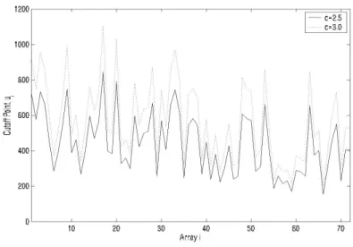
An implicit assumption in developing the thresholding algorithm is that small expression values are the noise values; however, “small” is relative to the array. That is, the noise level is array-specific. The question is how small is small (for each array)? The answer is the cutoff u at convergence, which separates noise values from “real” expressed values. This depends on the parameter c, the number of median absolute deviation above the median. Increasing c corresponds to a more stringent standard, since expression values must be larger to be excluded from the noise set. Since the resulting cutoff point does not depend on q, we set q=10% and ran the thresholding algorithm for c=2.5 and 3. The results are given in Figure 1. The pattern of
ui for c=3.0 and ui for c=2.5 is similar (Figure 1). Also evident from Figure
1 is that the estimate of array-specific noise varies a lot from one array to another. Therefore, it may not be optimal to use a single threshold value across all arrays and the thresholding algorithm avoids this.
Figure 1. Cut off point for c = 2.0 and 3.0.
Although the example given here consists of high-density oligonucleotide arrays, the thresholding algorithm can be applied to cDNA arrays as well. Assume that after background subtraction we have intensity measurements
for the red-fluorescent dye Cy5 and another for the green-fluorescent dye Cy3 for ith array. One strategy is to apply the above procedure to each set of dye measurements separately. After separate rescaling based on separate noise estimates for each channel, one can proceed to analyze the log(Cy5/Cy3) (positive) measurements. The reason for the separate applications of the thresholding algorithm to the sets of measurements from different channels is that the level of noise may be channel-specific.
DIMENSION REDUCTION: PARTIAL LEAST SQUARES
After array rescaling we examined dimension reduction methods to reduce the high p-dimensional gene space to a lower dimensional gene component space which can predict leukemia classes well. Some aspects of PLS are similar to principal component analysis (PCA), so we briefly review PCA. PCA is well known and is a commonly used dimension reduction method. Let X denote a data matrix of N rows, where each row consists of p gene expression values from a particular microarray experiment. (Thus, there are N samples or experiments.) Since the data dimension p is too large for many conventional statistical tools to be applied, PCA attempts to reduce this high gene dimension, p, to a much lower dimension, say K (K < N). This is achieved by extracting K gene components which are linear combinations of the original p genes. The components are extracted sequentially by maximizing the objective criterion, var(Xc), subject to orthogonality and norming constraints on the unit weight vector c. Very roughly, the constructed components summarized as much of the information (variation) of the original p genes, irrespective of response (leukemia) class information.Note that maximizing the variance of the linear combination of the genes, namely var(Xc), may not necessarily yield components predictive of leukemia classes. For this reason, a different objective criterion for dimension reduction (i.e., for selecting gene components) may be more appropriate for prediction of leukemia classes, for instance. The criterion for selecting gene components in PLS is to sequentially maximize the
covariance between the leukemia classes and a linear combination of the p
genes (also subject to orthogonality and norming constraints). That is, find the gene component weights, w, such that cov(Xw, y) is maximum, where y is the response vector of leukemia classes. We note that in PCA, the leukemia class information (y) was not used in constructing the gene components.
Based on the different objective criterion of PCA and PLS (namely var(Xc) and cov(Xw, y)) it is reasonable to suspect that if the original p
genes are predictive of the leukemia classes, then the constructed components from PCA would likely be good predictors of leukemia classes. Therefore, prediction results should be similar to that based on PLS gene components. Otherwise, PLS should perform better than PCA in predicting leukemia classes. The results based on the leukemia data given in the next section will support that this is indeed the case.
After dimension reduction by PLS (or PCA), the high dimension of p is reduced to a lower dimension of K gene components. We constructed K=3 gene components and predicted the leukemia classes based on the 3 components. (One can choose K, for example, by cross-validation. This was done but the final results did not change much so we choose the simpler model with K=3.) Since the reduced gene dimension is now low, conventional classification methods such as logistic discrimination and QDA (Quadratic Discriminant Analysis) can be applied. For an introduction to classical discrimination and classification the reader is referred to Flury (1997), Johnson and Wichern (1993), Mardia et al. (1979), and Press (1982). Details of LD (Logistic Discrimination) using PLS components including simulation results can be found in [Nguyen and Rocke, 2001].
RESULTS
Classification Based on 50 Predictive Genes
Although PLS can handle the number of genes, p, as large as expected in the human genome, experience indicates that prediction results are much improved when a subset of predictive genes are selected for the actual prediction or classification [Nguyen and Rocke, 2001]. This approach is reasonable since only a subset of the genes (probes) deposited on the array for investigation is predictive of the biological classes. For this reason and also for comparison purposes we first analyse the same p=50 genes obtained by Golub et al. (1999).
We constructed 3 gene components using PLS and PCA based on p=50 genes. Classification of the leukemia classes using the constructed gene components in logistic discrimination and quadratic discriminant analysis are compared. In this analysis we used the same set of 50 genes reported by Golub et al. as predictive of acute leukemia classes. That is, Golub et al. defined P(G, Y) = (m1 – m2)/(s1 + s2) as a measure of “correlation” (or
“distance”) between gene Gj and the class indicator variable Y, where mk and sk, k = 1, 2, are the sample means and standard deviations of the log of the expression levels of gene j in class 1 and 2 respectively. Twenty-five genes closest to class 1 and another twenty-five genes closest to class 2 were
selected to form a set of 50 “informative” genes. These are the selected predictors. Based on these 50 genes we carried out the following analysis steps:
1. Apply the thresholding algorithm to each array for (multiplicative) rescaling.
2. After rescaling, select the same 50 genes as in Golub et al. 3. Construct PLS components and PCs based only on the original 38
training samples.
4. Construct test components based on training component information. 5. Predict leukemia classes by (1) LD and (2) QDA using leave-one-out
cross-validation (CV) for the 38 training samples and then make out-of-sample predictions for the 34 test out-of-samples based on the constructed components from training information.
Leave-one-out CV predictions of the 38 training samples using QDA and LD with PLS gene components resulted in 100% correct and 36/38 for PCs. Based only on the training components, out-of-sample predictions for the 34 test samples were made. LD with PLS gene components resulted in one misclassification. Five test samples with low “prediction strength” (PS, defined in Golub et al.), samples # 54, 57, 60, 67, and 71 (with PS=0.23, 0.22, 0.06, 0.15, and 0.30), and one misclassified by Golub et al. were correctly classified with estimated conditional class probabilities of 0.97, 1.00, 0.98, 0.89, and 1.00. The second misclassified sample (# 66) by Golub et al. was the single misclassification by LD using PLS gene components. (This was the same sample misclassified by all CAMDA’00 conference participants.) LD using PCs did not predict the test sample well (with 7 incorrect). However, QDA using PLS components or PCs both had three misclassifications in the test samples.
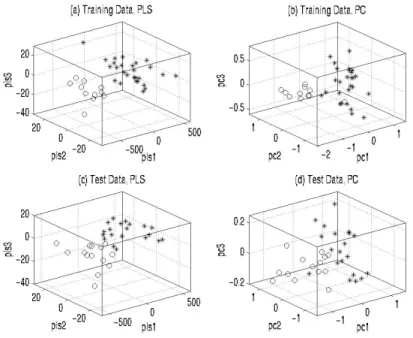
Figures 2(a)-(d) shows how the three constructed PLS gene components and PCs separate the leukemia classes in the training and test data. It can be seen that PLS components separate the leukemia classes better than PCs.
Assessment of Constructed Components for Classification
To assess the performances of (1) the various component construction methods and (2) the classification methods (LD and QDA), re-randomization is necessary. (Re-randomization was not considered by Golub et al. so a comparison here is not possible.) We considered a re-randomization scheme with equal splitting of the 72 samples into 36 training samples and the remaining 36 into test samples. The analyses above were repeated for 50 re-randomizations and the results indicate that the prediction based on the 50
Figure 2. Separability of leukemia samples in the training and test data sets by three gene
components extracted by PLS and PCA.
genes is stable--it is unlikely that the results depend on the original data configuration of 38 training/34 test samples split. The average percentages of correct classification over 50 re-randomizations are given in Table 1. Note that for each of the 50 randomizations (data sets), the prediction for the 36 training samples is based on leave-one-out CV and prediction for the remaining 36 test samples are based on out-of-sample prediction. Based on the 50 re-randomizations, PLS gene components performed at least as well or better than PCs on the training data for all (50/50) re-randomizations. This is based on leave-one-out CV. For the out-of-sample prediction of the test samples, PLS predicted at least as well or better than PCs in 42/50 re-randomizations.
Table 1. Average percentage correct in 50 re-randomizations.
LD LD QDA QDA
PLS PC PLS PC
Training Data 99.56 96.44 99.56 97.00
A Condition When PCs Fail to Predict Well
Attempts have been made to study the settings where PLS will predict well relative to other prediction methods, however, the conditions under which PLS predicts well have not been fully characterized in the statistics or chemometrics literature. The leukemia data set of Golub et al. provides an example of a condition under which PLS performs well relative to PCA. In the analyses given above, although the results for PLS components were better than that for PCs, the results for PCs were competitive nonetheless. Examining the objective criterion of PLS and PCA, we noted in section 2 that it would be reasonable to expect prediction based on PCs to be similar to that from PLS if the original genes are highly predictive of leukemia classes. This is the case of the analyses based on the 50 predictive genes. However, to see when PCs fail to predict well, while PLS components succeeded, we consider their prediction ability based only on expressed genes, but not expressed differentially for leukemia classes. This test condition is based on the simple fact that an expressed gene does not necessarily qualify as a good predictor of leukemia classes. For instance, consider a gene highly expressed across all samples, ALL and AML. In this case, the gene will not discriminate between ALL and AML well.
We define a gene to be expressed if the measure expression value is above the threshold value u determined from the thresholding algorithm (with parameter q=10% and c=3.0) as described in section 2. After rescaling, subset of p genes were retained for analysis. We analyzed five (nested) sets of genes defined as expressed on (A) at least one array (p=1,554), (B) 25% (p=1,076), (C) 50% (p=864), (D) 75% (p=662) and (E) 100% (p=246) of the arrays. As before, we applied PLS and PCA to extract gene components from these five data sets based on the 38 training samples. Predictions of the 38 training samples were based on leave-one-out CV and predictions of the 34 test samples were based on the training components only. This leads to a drastic decrease in performance of PCs relative to PLS. (Results not given here. For details, see Nguyen and Rocke (2001).)
To assess whether the observed decrease in performance of PCs relative to PLS gene components is coincidental, we considered a re-randomization study as in the analysis of the 50 informative genes. PCs did much worse relative to PLS gene components in the re-randomizations as well. The result here is not surprising since PCA aims to summarize only the variation of the
p genes. These p genes are above the threshold and therefore considered
expressed. However, only a subset of p expressed genes are predictive of leukemia classes. Why then does PLS components still perform well in this mixture of expressed genes, both predictive and non-predictive of leukemia classes? This is most likely attributed to the choice of objective criterion
used, namely covariation between the leukemia classes and (the linear combination of) the p genes. Since PLS components are obtained from maximizing cov(Xw, y) it is more able to assign pattern of weights to the genes which are predictive of leukemia classes. Details of the re-randomization study can be found in Nguyen and Rocke (2001).
CONCLUSIONS
In this paper we have presented a thresholding algorithm for estimating the array-specific noise and outlined rescaling procedure based on information from the thresholding algorithm. The algorithm is robust to outlying observations and is not affected by starting values (q). For example, we have applied the algorithm to the leukemia data set of Golub et al. We also described the use of the thresholding algorithm for cDNA arrays. After array rescaling, we introduced the use of PLS as a dimension reduction method for the analysis of gene expression data and illustrated the method’s effectiveness in predicting leukemia classes. Specifically, we have provided examples on the use of PLS gene components for classifying leukemia classes by quadratic and logistic discriminant analysis. The classification results are favorable when compared to the original results of Golub et al., as well as those based on PCs. These results hold under re-randomization studies as well. Finally, we have described a condition under which PLS components are superior to PCs for prediction purposes.
DISCUSSION
Easy Data Set?
It is now well known (CAMDA’00 conference) that the leukemia data set is an easy data set. That is, the leukemia classes are easily separable with the exception of one sample in the test data set. Nonetheless, the data set exhibits interesting characteristics that led to an elucidation of PLS and PCA for the analysis of microarray data. However, we have found similar successes with PLS in other data sets as well. Additional examples of cancer classifications, including normal versus ovarian tumor, diffuse large B-cell lymphoma versus B-cell chronic lymphocytic leukemia, normal versus colon tumor, and non-small-cell-lung-carcinoma versus renal samples, using PLS gene components can be found in Nguyen and Rocke (2001). Furthermore,
the method performs well under a simulation model for gene expression data [Nguyen and Rocke 2000, 2001b, 2001c].
Potential Applications of PLS to Microarray Data
Much published work in the analysis of gene expression data focuses on clustering genes. One motivation for the use of clustering is that “similar” gene expressions that are clustered together have similar functions, hence providing clues to gene functions. In addition to the wide use of clustering, we will discuss some other applications for microarray data in this section. Another area of interest (currently not as popular as clustering genes) may be the prediction of the expression of a target gene. Quantifying the predicted gene expression values such that they are compatible with some clinical outcomes is one use of this PLS prediction. Another use involves gene expressions measured over time. PLS prediction can be used to predict a target gene (or a cluster of target genes) over time. The goal of such an analysis may be to see which genes are related to the target gene and how this relationship varies with time.
Assessing the relationship between cellular reaction to drug therapy and their gene expression pattern is another application. For example, Scherf et al. (2000) assessed growth inhibition from tracking changes in total cellular protein (in cell lines) after drug treatment. The response of cell lines to each drug treatment can be considered as the response variables. Associated with the cell lines are their gene expressions. Since the expression patterns are from those of untreated cell lines, Scherf et al. focused on the relationship between gene expression patterns of the cell lines and their sensitivity to drug therapy. This relationship can be studied via a direct application of univariate or multivariate PLS, which can handle the high dimensionality of the data.
Another example, in cancer research, is the prediction of patient survival based on gene expressions. However, here some of the observed times are censored. Based on a simulation model of gene expression data, Nguyen and Rocke (2000c) studied various dimension reduction strategies involving PLS and PCA in the context of survival data with gene expressions as covariates. The results based on PLS are favorable based on this preliminary simulation study.
Finally, since many classification problems involve more than two classes, such as the classification of various types of tumors (leukemia, breast, renal, central nervous system, etc.), generalization to more than two classes is needed. Preliminary study of multivariate PLS for predicting multiple classes under a simulation model for gene expression data indicates that the method is useful [Nguyen and Rocke, 2000b].
PLS Algorithm and Computing Feasibility
One clear advantage of PLS over other dimension reduction method, such as PCA, is its computational feasibility. PLS components can be constructed in a few seconds, despite the high dimension p. Other dimension reduction methods, such as PCA, are much more computationally intensive when p is in the thousands. The PLS algorithm can be found, for instance, in Helland (1988), Hoskuldsson (1988), or Martens and Naes (1989).
ACKNOWLEDGMENTS
The research reported in this paper was supported by grants from the National Science Foundation (ACI96-19020, and DMS 98-70172), the National Institute of Environmental Health Sciences, National Institutes of Health (P43ES04699) and the National Cancer Institute (CA-90301). We thank the editors for comments that improved the presentation and content of the paper.
REFERENCES
Alon et al. (1999), “Patterns of Gene Expression Revealed by Clustering Analysis of Tumor and Normal Colon Tissues Probed by Oligonucleotide Arrays,” Proceedings of the
National Academy of Sciences, 96, 6745-6750.
Alizadeh et al. (2000), “Distinct Types of Diffuse Large B--Cell Lymphoma Identified by Gene Expression Profiling,” Nature, 403, 503-511.
Bittner et al. (2000), “Molecular Classification of Cutaneous Malignant Melanoma by Gene Expression Profiling,” Nature, 406, 536-540.
de Jong, S. (1993), “SIMPLS: An Alternative Approach to Partial Least Squares Regression,”
Chemometrics and Intelligent Laboratory Systems, 18, 251-263.
Dudoit, S., Fridlyand, J., Speed, T.P. (2000), “Comparison of Discrimination Methods for the Classification of Tumors Using Gene Expression Data,” Technical Report # 576, Department of Statistics, U. C. Berkeley.
Flury, B. (1997), A First Course in Multivariate Analysis. Springer-Verlag, New York. Frank, I.E., and Friedman, J.H. (1993), “A Statistical View of Some Chemometric Regression
Tools” (with discussion), Technometrics, 35, 109-148.
Garthwaite, P.H. (1994), “An Interpretation of Partial Least Squares,” Journal of the
American Statistical Association, 89, 122-127.
Geladi, P., and Kowalski, B.R. (1986), “Partial Least Squares Regression: Tutorial,”
Analytica Chimica Acta, 185, 1-17.
Golub et al. (1999), “Molecular Classification of Cancer: Class Discovery and Class Prediction by Gene Expression Monitoring,” Science, 286, 531-537.
Hand, J.D. (1981), Discrimination and Classification. John Wiley Sons, Chichester, England. Hand, J.D. (1997), Construction and Assessment of Classification Rules. John Wiley Sons,
Helland, I.S. (1988), “On the Structure of Partial Least Squares,” Communications in
Statistics-Simulation and Computation, 17, 581-607.
Helland, S., and Almoy, T. (1994), “Comparison of Prediction Methods When Only a Few Components are Relevant,” Journal of the American Statistical Association, 89, 583-591. Hoskuldsson, A. (1988), “PLS Regression Methods,” Journal of Chemometrics, 2, 211-228. Johnson, R.A. and Wichern, D.W. (1992), Applied Multivariate Analysis. Prentice-Hall, New
Jersey, 4th edition.
Jolliffe, I.T. (1986), Principal Component Analysis. Springer-Verlag, New York.
Lorber, A., Wangen, L.E., and Kowalski, B.R. (1997), “A Theoretical Foundation for the PLS Algorithm,” Journal of Chemometrics, 1, 19-31.
Mardia, K.V., Kent, J.T., and Bibby, J..M. (1979), Multivariate Analysis. Academic Press, London.
Martens, H. and Naes, T. (1989), Multivariate Calibration, John Wiley Sons, New York. Massey, W.F. (1965), “Principal Components Regression in Exploratory Statistical
Research,” Journal of the American Statistical Association, 60, 234-246.
Nguyen, D.V. and Rocke, D.M. (2000), “Classification in High Dimension with Application to DNA Microarray Data,” manuscript.
Nguyen, D.V. and Rocke, D.M. (2001), “Tumor Classification by Partial Least Squares Using Microarray Gene Expression Data,” to appear in Bioinformatics.
Nguyen, D.V. and Rocke, D.M. (2001b), “Partial Least Squares Proportional Hazard Regression for Application to DNA Microarray Data,” manuscript.
Nguyen, D.V. and Rocke, D.M. (2001c), “Multi-Class Cancer Classification Via Partial Least Squares Using Gene Expression Profiles,” manuscript.
Perou et al. (2000), “Molecular Portrait of Human Breast Tumors,” Nature, 406, 747-752. Perou et al. (1999), “Distinctive Gene Expression Patterns in Human Mammary Epithelial
Cells and Breast Cancer,” Proceedings of the National Academiy of Sciences, USA, 96, 9112-9217.
Phatak, A., and Reilly, P.M., and Penlidis, A. (1992), “The Geometry of 2-Block Partial Least Squares,” Communications in Statistics-Theory and Methods, 21, 1517-1553.
Press, S.J. (1982), Applied Multivariate Analysis: Using Bayesian and Frequentist Methods of
Inference. Robert E. Krieger Publishing Company Inc., Malabar, Florida, 2nd edition.
Rocke, D.M. and Durbin, B. (2000), “A Model for Measurement Error for Gene Expression Arrays,” to appear in Journal of Computational Biology.
Ross et al. (2000), “Systematic Variation in Gene Expression Patterns in Human Cancer Cell Lines,” Nature Genetics, 24, 227-235.
Scherf et al. (2000), “A Gene Expression Database for the Molecular Pharmacology of Cancer,” Nature Genetics, 24, 236-244.
Stone, M., and Brooks, R. J. (1990), “Continuum Regression: Cross-validated Sequentially Constructed Prediction Embracing Ordinary Least Squares, Partial Least Squares, and Principal Components Regression” (with discussion), Journal of the Royal Statistical