ISSN: 2502-4752, DOI: 10.11591/ijeecs.v17.i2.pp1117-1126 1117
Rainfall-runoff modelling using adaptive neuro-fuzzy
inference system
Nurul Najihah Che Razali1, Ngahzaifa Ab. Ghani2, Syifak Izhar Hisham3,
Shahreen Kasim4, Nuryono Satya Widodo5, Tole Sutikno6
1,2,3Faculty of Computer Systems & Software Engineering (FSKKP), Universiti Malaysia Pahang, Malaysia 4Faculty of Computer Science & Information Technology, Universiti Tun Hussein Onn Malaysia, Malaysia
5,6Faculty of Industrial Technology, Universitas Ahmad Dahlan, Yogyakarta, Indonesia
Article Info ABSTRACT
Article history: Received Jul 9, 2019 Revised Oct 2, 2019 Accepted Oct 13, 2019
This paper discusses the working mechanism of ANFIS, the flow of research, the implementation and evaluation of ANFIS models, and discusses the pros and cons of each option of input parameters applied, in order to solve the problem of rainfall-runoff forecasting. The rainfall-runoff modelling considers time-series data of rainfall amount (in mm) and water discharge amount (in m3/s). For model parameters, the models apply three triangle membership functions for each input. Meanwhile, the accuracy of the data is measured using the Root Mean Square Error (RMSE). Models with good performance in training have low values of RMSE. Hence, the 4-input model data is the best model to measure prediction accurately with the value of RMSE as 22.157. It is proven that ANFIS has the potential to be used for flood forecasting generally, or rainfall-runoff modelling specifically.
Keywords: Rainfall-runoff ANFIS
Artificial intelligence Forecasting
Copyright © 2020 Institute of Advanced Engineering and Science. All rights reserved.
Corresponding Author: Nurul Najihah Che Razali,
Faculty of Computer Systems & Software Engineering (FSKKP), Universiti Malaysia Pahang,
Lebuhraya Tun Razak, 26300, Kuantan, Pahang Darul Makmur, Malaysia. Email: [email protected]
1. INTRODUCTION
Nowadays, the flood is a common natural disaster in Malaysia, which happens almost every year during the monsoon season. Normally, the factors of flood occurrences such as heavy monsoon rainfall, strong convection rain storms, poor drainage, and other local factors. Each season, flood is major, critical and unpredictable problem. This leads to a significant loss of lives, damage to crops, livestock, property, and public infrastructure.
In Kuantan, population of flood victims with 2,976 people from 841 families were looking for a place to take shelter at 17 relief centres in November, 2018 [1]. As in previous years, Kuantan constant to be the worst hit district in Pahang based on the Welfare Department’s official flood portal. In the meantime, other districts in Pahang also involved with flood. There were 1,392 victims from 349 families in Pekan, 141 people from 35 families in Bera, 110 people from 31 families in Maran and five victims from three families in Temerloh [1]. Early of this year, according to the Drainage and Irrigation Department (DID) website, it showed Sungai Lepar Station at Gelugor Bridge (30.34 metres) and Sungai Belat Station at Sri Damai (5.83 metres) had exceeded the level of danger point. While, Sungai Pahang Station at Paloh Hinai (9.78m), Sungai Tembeling at Kuala Tahan (67.73 metres), Sungai Pahang at Sungai Yap (51.95m) and Sungai Kuantan at Pasir Kemudi (7.84m) showed warning-level evaluations [2].
Since the early 1990s, artificial intelligence has been widely explored as modelling tools. One of the well-known models is Adaptive Neuro-Fuzzy Inference System or ANFIS. ANFIS is a kind of artificial neural network that is based on Takagi-Sugeno fuzzy inference system. Prediction for rainfall is not easy. It must
measure many things such as space and time scale. Researchers consider rainfall as a stochastic process [3-6]. There are some works by researchers produced output for forecasting using ANFIS [7]. The measurement parameters for rainfall forecasting are weather prediction [8], wind speed [9], river flow estimation [10], and simulation for daily temperature [11]. In this work, a model based on ANFIS shall be developed based on time-series data of rainfall amount (in mm) and water discharge amount (in m3/s). The working mechanism of ANFIS is further explained in Section 2 (2.2).
2. RESEARCH METHOD
2.1. The process of ANFIS Modelling for Rainfall-Runoff
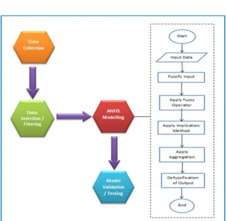
In order to implement and evaluate the accuracy of ANFIS model, this research is done according to these research activities – data collection, data selection, ANFIS implementation, and model validation. This is summarized in the flow chart in Figure 1.
Figure 1. Process flow of ANFIS modelling for rainfall-runoff
Dataset was collected from the Department of Irrigation and Drainage Malaysia. The collected dataset is of seven years, namely from 2009 to 2014. This set of data is selected mainly because of the extreme values from 2013, the most recent big flood in Kuantan. Then, the dataset must be selected and filtered before it can be used to implement ANFIS. This is to avoid false result and minimize errors. After the filtering process, the data is trained with ANFIS in order to produce the trained ANFIS model. Finally, the model output is then tested and compared with the observed values.
2.2. The Working Mechanism of ANFIS
In ANFIS, there are six processes to produce data to get an accuracy output using values as providing from Hydrology Department. Figure 2 shows how ANFIS works (based on MATLAB Fuzzy Logic Toolbox). The rainfall runoff data Kuantan is put to proceed to the next process. The steps are explained in Figure 2.
Figure 2. The working mechanism of ANFIS
STEP 1: FUZZIFY INPUT
Input is fuzzified using trimf (Triangle Membership Function) known as the process of defining the membership degree by using the membership function of each variable.
STEP 2: APPLY FUZZY OPERATOR
After fuzzified input is processed, the rules are identified for each membership degree. In rules, it must have an operator (AND, OR, NOT) if antecedents are more than one. The operation ‘AND’ is applied in a combination of two antecedents to produce weight.
STEP 3: APPLY IMPLICATION METHOD
The output from step 2, which is the weight for each rule, is used to apply the implication method to produce normalized weight. Then, each rule will get its own normalized weight once the implication method has been applied wisely.
STEP 4: APPLY AGGREGATION
As a result of the implication method application in Step 3, each rule (Rule 1, Rule 2, Rule 3 and Rule 4) has its own weighted values with the normalized weight. Hence, there are four weighted values done.
STEP 5: DEFUZZICATION OF OUTPUT
The output of the previous process (Step 4) is the combined membership functions from all rules. Therefore, in the defuzzification of the output process, all weighted rules are combined in order to produce final outputs.
2.3. How ANFIS Process Data
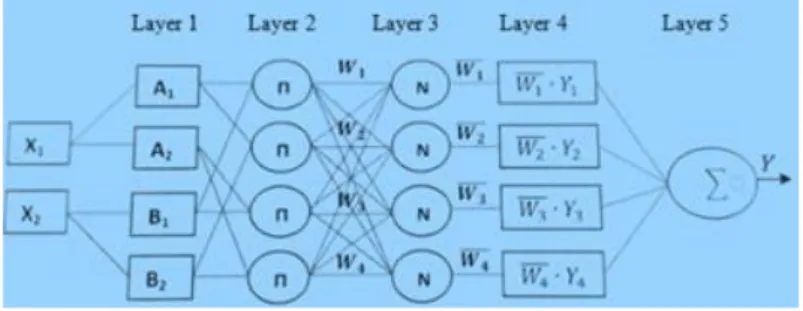
Figure 3. ANFIS architecture for a two-input model [11]
Let the example dataset is obtained by the equation [12]: 𝑌 = 1
𝑋1+ 𝑋2
2 (1)
where X is parameter for trimf, and Y is rainfall runoff parameter.
Where 𝑋1= 6 and 𝑋2= 0.4761 as inputs and Y is 0.39338 as output. In step 1, let the type of
membership function applies trimf (triangular membership function), this triangular shape membership function is a function of the input vector based on three parameters a, b and c as listed it Table 1. The membership degree, or weight (w), is calculated using equations as [3]
𝐼𝑓 𝑋𝑖 ≤ 𝑎 𝑡ℎ𝑒𝑛 𝑤𝑖= 0 (2) 𝐼𝑓 𝑎 ≤ 𝑋𝑖 ≤ 𝑏 𝑡ℎ𝑒𝑛 𝑤𝑖= 𝑋𝑖−𝑎 𝑏−𝑎 (3) 𝐼𝑓 𝑏 ≤ 𝑋𝑖 ≤ 𝑐 𝑡ℎ𝑒𝑛 𝑤𝑖= 𝑐−𝑋𝑖 𝑐−𝑏 (4) 𝐼𝑓 𝑋𝑖 ≥ 𝑐 𝑡ℎ𝑒𝑛 𝑤𝑖= 0 (5)
where a, b, c are rainfall parameters and w is water discharge parameter.
After identifying the equations as required, replaced all input values in the equations as: 𝐴1, 𝑐−𝑋1 𝑐−𝑏 = (10.01−6) (10.01−0.9539)= 0.4428 𝐴2, 𝑋1−𝑎 𝑏−𝑎 = (6−0.9998) (9.9540−0.9998)= 0.5584 𝐵1, 𝑐−𝑋1 𝑐−𝑏 = (0.9388−0.4761) (0.9388−0.2948)= 0.7185 𝐵2, 𝑋1−𝑎 𝑏−𝑎 = (0.4761+0.1849) (1.1030+0.1849)= 0.5132
From the calculation above, we produce shapes which contribute in obtaining membership degree as provided in Table 1.
Table 1. Parameters for Trimf for X1=6 and X2=0.4761
a b c w
A1(mf for X1) −8 0.9539 10.01 0.4428
A2(mf for X1) 0.9998 9.9540 19 0.5584
B1(mf for X2) −0.9316 0.2948 0.9388 0.7185
B2(mf for X2) −0.1849 1.1030 1.939 0.5132
In layer 2, the membership degrees of both X1 and X2are combined with the fuzzy operator AND
A1 and B2. The AND operator is equivalent to multiplication operation. Therefore, the outputs of layer 2 are
obtained by multiplying the weight as equations below.
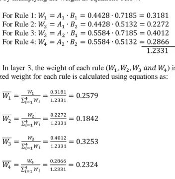
For Rule 1: 𝑊1 = 𝐴1∙ 𝐵1= 0.4428 ∙ 0.7185 = 0.3181
For Rule 2: 𝑊2 = 𝐴1∙ 𝐵2 = 0.4428 ∙ 0.5132 = 0.2272
For Rule 3: 𝑊3 = 𝐴2∙ 𝐵1 = 0.5584 ∙ 0.7185 = 0.4012
For Rule 4: 𝑊4= 𝐴2∙ 𝐵2= 0.5584 ∙ 0.5132 = 0.2866
1.2331
In layer 3, the weight of each rule (𝑊1, 𝑊2, 𝑊3 𝑎𝑛𝑑 𝑊4) is normalized to the sum of the weight. The
normalized weight for each rule is calculated using equations as: 𝑊1 ̅̅̅̅ = 𝑊1 ∑4𝑖=1𝑊𝑖 =0.3181 1.2331= 0.2579 (6) 𝑊2 ̅̅̅̅ = 𝑊2 ∑4𝑖=1𝑊𝑖= 0.2272 1.2331= 0.1842 (7) 𝑊3 ̅̅̅̅ = 𝑊3 ∑4𝑖=1𝑊𝑖 =0.4012 1.2331= 0.3253 (8) 𝑊4 ̅̅̅̅ = 𝑊4 ∑4𝑖=1𝑊𝑖= 0.2866 1.2331= 0.2324 (9)
In layer 4, the normalized weight for each rule is multiplied with a linear function associated with the rule to get the sub-output. The calculation is done as in equations below. The process is equivalent to the process of ‘aggregation of the consequents’ in the fuzzy inference system.
𝜃𝑅𝑢𝑙𝑒 1: 𝑊̅̅̅̅ ∙ 𝑌1 1= 0.2579 ∙ 0.8447 = 0.2178 (10)
𝜃𝑅𝑢𝑙𝑒 2: 𝑊̅̅̅̅ ∙ 𝑌2 2= 0.1842 ∙ 1.012 = 0.1864 (11)
𝜃𝑅𝑢𝑙𝑒 3: 𝑊̅̅̅̅ ∙ 𝑌3 3= 0.3253 ∙ (−0.09979) = −0.0324 (12)
𝜃𝑅𝑢𝑙𝑒 4: 𝑊̅̅̅̅ ∙ 𝑌4 4= 0.2324 ∙ (−0.0925) = −0.0214 (13)
Finally, in layer 5, the defuzzification process is done when all sub-outputs are combined to get one final crisp output as below.
𝑌 = 𝜃𝑅𝑢𝑙𝑒 1+ 𝜃𝑅𝑢𝑙𝑒 2+ 𝜃𝑅𝑢𝑙𝑒 3+ 𝜃𝑅𝑢𝑙𝑒 4 = 0.3504
2.4. Modelling of Dataset
In the set of data have two variables are used, water discharge (Q) and rainfall (R). In this modelling, it experiments the variables by set or group. Table 2 shows, there are four sets of data that have been modelled using ANFIS. After filtering the dataset, the data is ready to be loaded by ANFIS toolbox. The sets of data are as in Table 2.
Table 2. Modelling of the Dataset
Dataset Input Output
One Input R(t) Q(t)
Two Input R(t).Q(t-1) Q(t)
Three Input R(t).R(t-1).Q(t-1) Q(t)
Four Input R(t).R(t-1).R(t-2).Q(t-1) Q(t)
The unit of measurement of dataset for water discharge (Q) is m3/s and for rainfall (R) mlare used. R(t) is current day for rainfall, R(t-1) is known as a previous day for rainfall and R(t-2) represent for previous two days. Additionally, Q(t) is current day for water discharge, also known as output, Q(t-1) represents the previous day for water discharge.
3. RESULTS & DISCUSSION
3.1. The result of Dataset with Scatter Plot
The final results of prediction have been explained in this section, it provides four figures to describe the results of four datasets that have been modelled. Each figure has observed data as x-axis versus predicted data as y-axis. It shows R squared (R2), also known as the coefficient of determination, which is a statistical measure of how close the data to fit the regression line. In this case, the value of R2 is not directly a measure of how good the modelled values are, but instead a measure of how good a predictor might be constructed from the modelled values.
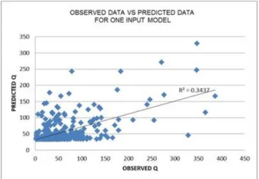
Figure 4 shows observed data versus predicted data for one input model, that scattered plot appearances very complex and get overfitted. The value of R2 = 0.3437, which is the smallest value compared to other models. Nevertheless, it does not mean the smallest value is the best model.
Figure 4. Observed data versus predicted data for 1-input model
Figure 5 shows ANFIS model on 2-input dataset, which the scattered plots are not complex and less overfitted. Besides, the coefficient of determination is R2 = 0.7311indicates that this model has higher value rather than R-squaredin 1-input data model.
Figure 5. Observed data versus predicted data for 2-input model
Figure 6 shows the scatterplots of R-squared for 3-input data model respectively. From the graph, R2 = 0.7924 where the value is higher than Figure 4 and Figure 5. This graph shows that the model has poor overfitted plots which mean it is a good model because the plots are near to the outliers.
Figure 6. Observed data versus predicted data for 3-input model
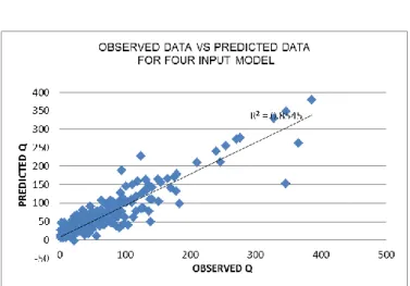
By comparing the scatter plots between models, Figure 7 is chosen as the best design because the overfittings of the model are not obvious. The coefficient of determination (R2) shows the 4-input model is has the highest value which is 0.88545. Even though this model is less over-fitted and has the highest R-squared, it is not described as having perfect accuracy of prediction. The accuracy will be measured by Root Mean Square Error (RMSE) which will be explained for next section.
Figure 7. Observed data versus predicted data for 4-input model
3.2. The Best Output with Root Mean Square Error
In this section, four models are defined based on the performance of models on both training and testing datasets already considered about over-fitted, R-squared and line of regression. While the R-squared is a relative measure, the RMSE is an absolute measure of prediction accuracy.
RMSE is the square root of the variance of the residuals. It indicates how close the observed data points are to the model’s predicted values. Lower values of RMSE indicate better accuracy. RMSE is a good measure of how accurately the model predicts the response and is the most important criterion for fit if the main purpose of the model is prediction [13].
Table 3 shows data of four models with R-squared values and values of RMSE as mainly have been defined.
Table 3. Comparisons of Root Mean Square Error and R Squared
Dataset / Measurement One Input Two Input Three Input Four Input
R² 0.3437 0.7311 0.7924 0.8545
RMSE = √1
𝑛∑ (𝑦𝑖− 𝑦̂𝑖) 𝑛
𝑖=1 ² (9)
where yi = expected values, ŷi= observed values and n=sample values, that has produced values RMSE for each model. The model with the lowest value of RMSE has the best performance. Based on Table 3, the 4-input model has the lowest RMSE value thus it is the best model to measure an accuracy in prediction, with less over fitted plots and the highest value of R-squared.
3.3. Comparison of ANFIS Model with Conventional Methods
In this section, an ANFIS model is compared with the conventional method. A selected of the conventional method in this experiment is Multiple Linear Regression (MLR) which the tool was applied by Waikato Environment for Knowledge Analysis (Weka). The Weka tool is a collection of machine learning algorithms for data mining tasks [13].
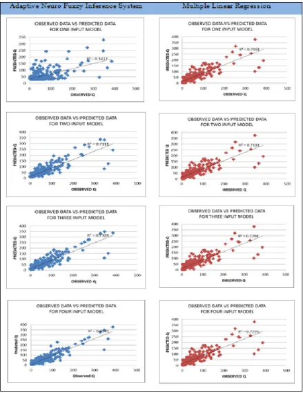
Figure 8 shows the comparison of results by the scattered plots of ANFIS model and MLR method. The accuracy can be described through the plot pattern which less overfitting brings the best result. The result from ANFIS looks better based on scattered plot and the plot location to the regression line. However, the figure also shows R Squared values of MLR method are all above 0.7.
Figure 8. Comparison between ANFIS and MLR
Table 4 shows the comparison of final result of ANFIS model and the MLR method. The Table 4 (a) and (b) consist of R Squared values and RMSE values of all datasets. The table shows a model trained with the same dataset for both methods. As can be seen in the table, the highest RMSE is 46.9650 for 1-input dataset
on ANFIS model but 1-input of MLR model is 42.6782. Therefore, the MLR model is appropriate for a simple problem or having less attributes.
Nonetheless, the 4-input dataset of ANFIS model records as 22.1570, which the lowest value of RMSE indicate better fit [14]. Definitely, ANFIS is appropriate for the complex problem while MLR is proved that it can apply better for one input as known as MLR is a simpler algorithm.
Table 4. Comparison of the Result ANFIS Model (a) and MLR Method (b) Method a ANFIS
Dataset / Measurement One Input Two Input Three Input Four Input
R² 0.3437 0.7311 0.7924 0.8545
RMSE 46.9650 29.4180 26.3290 22.1570
Method b MLR
Dataset / Measurement One Input Two Input Three Input Four Input
R² 0.7191 0.7191 0.7298 0.7295
RMSE 42.6782 30.0675 30.0415 30.2075
4. CONCLUSION
Rainfall is natural climate phenomena whose prediction is challenging and demanding. In the field of modeling and classification framework, there are many studies that use the Neuro-Fuzzy Approach and. The models have been developed for monthly precipitation forecasts using ANFIS [15-21].
The models that have been study in this paper are using adaptive neuro-fuzzy inference system with weather radar data to prove accuracy of prediction. It used object-based approach using the fuzzy logic, as well as segmentation technique and a feature extraction procedure has been developed [22]. For this reason, rainfall data and water discharge data are important to prediction of flood in Pahang. ANFIS is the most popular with other techniques because it has efficient function to get the output of experiment in study cases.
The ANFIS model is trained using rainfall-runoff data of Kuantan catchment. The accuracy of the models is measured using RMSE and R Squared. The good values of these two measures have been obtained from the 4-input model indicating that this is the best input combination for the rainfall-runoff model of Kuantan catchment. The result also shows that ANFIS has the potential to be used for flood forecasting generally, or rainfall-runoff modelling specifically.
5. OTHER RECOMMENDATIONS
Based on the findings of major flood in Pahang, it can be explored for another area in Pahang to measure the accuracy, for example, Temerloh, Raub, Maran, Cameron Highland and Jerantut. In short, it can measure the accuracy as long as the usability comes out in the techniques. In ANFIS, there are several membership functions. For this project, the triangle membership function was applied and other membership functions can be used, such as Gaussian membership function, Generalized Bell membership function, ‘Pi’ membership function, sigmoidal membership function and Trapezoidal membership function. The Gaussian memberships function in ANFIS is also commonly used in data predictions.
REFERENCES
[1] Fair weather improves Pahang flood situation, New Straits Times, 09 November, 2018. [2] Floods worsen in Pahang, over 1,800 evacuated, The Sun Daily, 03 January, 2018.
[3] P.K. Kundu, D.A. Marks, J.E. Travis, Statistical intercomparison of idealized rainfall measurements using a stochastic fractional dynamics model, J. Geophys. Res.-Atmos. 119, 10,139–110,159, 2014.
[4] N. Ramesh, R. Thayakaran, C. Onof, Multi-site doubly stochastic Poisson process models for fine-scale rainfall,
Stoch. Env. Res. Risk A., 27, 1383–1396, 2013.
[5] M.Schleiss, S.Chamoun, A.Berne, Stochastic simulation of intermittent rainfall using the concept of “dry drift”.
Water Resour. Res. 50, 2329–2349., 2014.
[6] R.Hashim, C.Roy, S.Motamedi, S.Shamshirband, D.Petković, M.Gocic & S.C.Lee, Selection of meteorological parameters affecting rainfall estimation using neuro-fuzzy computing methodology. Atmospheric Research, 171, 21– 30., 2016.
[7] A.Danladi, M.Stephen, B.M.Aliyu, G.K.Gaya, N.W. Silikwa & Y.Machael, Assessing the influence of weather parameters on rainfall to forecast river discharge based on short-term. Alexandria Engineering Journal, 0–5., 2017. [8] C. Fernando, J. Nickel, Average hourly wind speed forecasting with ANFIS, in: 11th Americas Conference on wind
Engineering – San Jaun Puerto Rico, 2009.
[9] Y.W. Khun, A study on soft computing approach in weather forecasting. Masters thesis, Universiti Teknologi Malaysia., 2010.
[10] O.E. Jaafer, S.A. Akrami, Adaptive neuro-fuzzy inference system based model for rainfall forecasting in Klang River, Malaysia, Int. J. Phys. Sci. 6 (12) 2875–2888., 2011.
[11] J. Yen, R. Langari, Fuzzy Logic, Intelligence, Control, and Information, Prentice Hall, 1999.
[12] N.A. Ghani, An evaluation of the potential of adaptive neuro-fuzzy inference system in hydrological modelling and prediction. PhD thesis, University of Nottingham., 2012.
[13] Z.Markov & I.Russell, An Introduction To The Weka Data Mining System. 2005. [14] K.G. Martin, Assessing The Fit Of Regression Models. 2005
[15] Pradip, Kyada & Kumar, Pravendra & M. A., Sojitra. Rainfall Forecasting Using Artificial Neural Network (Ann) And Adaptive Neuro-Fuzzy Inference System (Anfis) Models. International Journal of Agriculture Sciences. 10. 6153-6159, 2018.
[16] Aldrian E. and Djamil Y. S. Makara Journal of Science, 13,7-14, 2008.
[17] Bacanli U.G., Firat M. and Dikbas F. Stochastic Environmental Research and Risk Assessment, 23,1143-1154, 2009. [18] Tektas M. Environmental Research Engineering and Management, 51,5-10, 2010.
[19] Jeong C., Shin J., Kim T. and Heo J.H. Water Resource Management, 26(15),4467-4483, 2012.
[20] Darmawan, M. F., Jamahir, N. I., Saedudin, R. R., & Kasim, S. (2018). Comparison between ANN and Multiple Linear Regression Models for Prediction of Warranty Cost. International Journal of Integrated Engineering, 10(6). [21] Yahya, N. A., Samsudin, R., Darmawan, I., Shabri, A., & Kasim, S. (2018). Group Method of Data Handling with
Artificial Bee Colony in Combining Forecasts. International Journal of Integrated Engineering, 10(6).
[22] L.Pulvirenti, F.Marzano, N. Pierdicca, S.Mori & M.Chini (n.d.). Discrimination of Water Surfaces, Heavy Rainfall, and Wet Snow Using COSMO-SkyMed Observations of Severe Weather Events. IEEE Trans. Geosci. Remote Sensing IEEE Transactions on Geoscience and Remote Sensing, 858-869., 2014.