Integrating Deep Semantic Segmentation
into 3D Point Cloud Registration
Anestis Zaganidis
Li Sun
Tom Duckett
Grzegorz Cielniak
Abstract— Point cloud registration is the task of aligning 3D scans of the same environment captured from different poses. When semantic information is available for the points, it can be used as a prior in the search for correspondences to improve registration. Semantic-assisted Normal Distributions Transform (SE-NDT) is a new registration algorithm that reduces the complexity of the problem by using the semantic information to partition the point cloud into a set of normal distributions, which are then registered separately. In this paper we extend the NDT registration pipeline by usingPointNet, a deep neural network for segmentation and classification of point clouds, to learn and predict per-point semantic labels. We also present the Iterative Closest Point (ICP) equivalent of the algorithm, a special case of Multichannel Generalized ICP. We evaluate the performance of SE-NDT against the state of the art in point cloud registration on the publicly available classification data setSemantic3d.net. We also test the trained classifier and algorithms on dynamic scenes, using a sequence from the public datasetKITTI. The experiments demonstrate the improvement of the registration in terms of robustness, precision and speed, across a range of initial registration errors, thanks to the inclusion of semantic information.
I. INTRODUCTION
Point cloud registration is the alignment of 3D scans of an environment, consisting of points, that are captured from different locations. Common applications of scan registration are the construction of a 3D model of an object, a map of an environment, or the recovery of the pose transform of the sensor for self-localization. Algorithms that address the problem of registration approach it as an optimization problem of minimizing a distance metric between the scans, with respect to the 6-DOF transform. Popular techniques in-clude Generalized Iterative Closest Point (GICP) [1] and 3D Normal Distributions Transform (NDT) [2], [3]. These meth-ods can perform sufficiently well for autonomous robotic applications in enclosed spaces such as indoor environments, but their performance degrades in open environments with limited geometric structure.
In our previous work, we proposed the Semantic-assisted Normal Distributions Transform (SE-NDT) [4], a registration method that uses normal distribution transforms but also con-siders per-point semantic information that might be available to aid the registration process. An increasing number of robotic systems employ semantic segmentation algorithms for various purposes, for example, to detect traversable
Lincoln Centre for Autonomous Systems (LCAS), University of Lincoln,
This work has received funding from the European Unions Horizon 2020 research and innovation programme under grant agreement No 732737 (ILIAD).
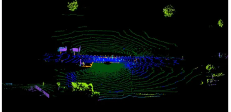
Fig. 1. An indicative point cloud from theSemantic3d.netdataset (’sg27 station 1’) as labeled by PointNet RGB.
terrain, buildings, trees, crops, etc. The output of those systems can be used, without additional cost, to improve localization or 3D model construction. However, we only provided a “proof of concept” for the algorithm by testing one continuous geometric measure of smoothness, which was used to partition the point cloud into two categories,edgeand planepoints.
In this work, we present a complete semantic registration pipeline, using PointNet [5] as the source of semantic labels. We train the semantic classifier on the manually labeled data setSemantic3d.net[6]. We also present the conceptual equivalent of our algorithm for GICP, referred to as SE-GICP. We evaluate the extended registration methods in comparison with GICP and NDT using the predicted semantic labels for scenes unseen before by the classifier. As only one, but detailed, scan is available per scene, we split each scan into several point clouds that simulate multi-scan data according to the specifications of a consumer Lidar sensor.
We compare SE-NDT, NDT, GICP and Fast Global Reg-istration [7] on the resulting data set and on KITTI [8] and demonstrate that SE-NDT outperforms the other methods in speed, robustness and precision.
II. RELATED WORK
Iterative Closest Point (ICP) is perhaps the most widely used scan registration method. The method was proposed in [9], and several extensions and generations have been pre-sented. In [10] the authors introduce probabilistic association in ICP, where instead of matching point-to-point, they use a
t-distribution to model the distances to a set of target points and assign a weight to each association. ICP iteratively finds point correspondences between point clouds and minimizes a distance cost function. A registration method that uses
semantic information to improve ICP was presented in [11] where the semantic categories used were floor points, ceiling points, wall points and artifact points. The authors noted a reduction in registration convergence time with no loss of quality, attributed to the raised probability of picking correct correspondences.
Fast Point Feature Histograms (FPFH) were introduced in [12] to provide initial alignment and possible corre-spondences to ICP. Even though the method does not use semantic information in the strict sense, the handling of the added information is similar. Fast Global Registration [7] (FGR) uses FPFH to find correspondences in feature space, that are further filtered to reduce incorrect matches. The algorithm can cope with noisy correspondences and therefore does not need to re-estimate them during optimization. The registration does not use an initial estimate, and an extension provides multi-scan registration.
The Normal Distributions Transform (NDT) is a method for 2D registration proposed in [2] that transforms the point clouds into sets of normal distributions, and iteratively finds point-to-distribution correspondences and minimizes a distance cost function. The method was extended to 3D in [3], and in [13] to use distribution-to-distribution correspon-dences and cost function.
Several approaches that integrate non-geometric informa-tion into NDT registrainforma-tion have been presented. In [14] two variations of NDT were presented that use colour information to improve registration. The method penalizes matches of non-corresponding colour with an additional error function and models the colour as additional dimensions on the Normal Distributions (6D). Another approach to improve NDT by using colour was presented by [15], where the con-tribution of every discon-tribution-to-discon-tribution correspondence is dependent on the colour similarity. The use of features instead of the full point cloud was exhibited by [16].
Semantic-assisted Normal Distributions Transform regis-tration (SE-NDT) [4], a method we introduced in our previ-ous work, uses semantic information to segment the point cloud and constructs the Normal Distributions Transform for each segment independently. Distribution-to-distribution correspondences are then only searched among the NDTs constructed from the same type of semantic label. Previously, we used a continuous geometric measure of smoothness as the source of semantic information, to segment the point cloud into two categories edge and plane. In this work, we introduce the use of real semantics, resulting from a classifier, by using PointNet [5], a deep-learning framework to learn semantic labels from data. In this paper, we examine the registration procedure by using the manually labeled data setSemantic3d.net[6].
III. REFERENCE REGISTRATION METHODS
A. Generalized ICP
The Generalized Iterative Closest Point (GICP) is a method introduced in [1] that unifies the point-to-point [9] and point-to-plane [17] iterative closest point algorithms and introduces plane-to-plane registration.
GICP approximates the transformation that aligns two point clouds by minimizing a distance function between point correspondences. To register a cloud M to a cloud
F the algorithm finds for each v ∈ M the closest point
uv ∈ F. The Euclidean distance measure is used. Point
correspondences above a maximum distance threshold are rejected. The transform T which aligns the two clouds is then obtained by minimizing the function
f(T) = X
v∈M
(uv−T v)(Cu+T CvTT)−1(uv−T v)T.
(1)
Cu and Cv are the covariance matrices of the assumed
surface containing the point. The assumed surface has the minimum variance in the direction of the normal, so the covariance can be represented in the form
Ci=Ri 0 0 0 1 0 0 0 1 R T i (2)
withRthe rotation that makesthe magnitude of the normal (whereis a very small constant). The procedure is repeated iteratively until a termination criterion is met, usually where the error is below a threshold or the number of iterations exceeds a limit.
B. 3D-NDT
Normal Distributions Transform (NDT) is a method for the representation of the environment and registration of data, proposed by Biber and Straßer [2] for 2D scan registration, and later extended for the registration of three-dimensional data by Magnusson et al. [3]. As opposed to other methods which use either a full point cloud or feature points to perform the registration, 3D-NDT assumes a local Gaussian distribution of points and uses the probability density func-tion as their representafunc-tion. Space is segmented into voxels, and for each voxel a Gaussian model is fitted to the data. In the point-to-distribution (P2D) variant, the registration of a new scan then becomes a problem of fitting its points to the distribution, which is solved as a least-squares problem.
The distribution-to-distribution variant of NDT [13], [18] consists of the following steps to register a point cloudM
to a point cloudF. At its first step, the algorithm discretizes the space into voxels. Let Si be the set of points v of F
in voxeli. A Gaussian distribution of points is assumed for every voxel, resulting in the sets of distributions GF,GM.
The mean vector µi and the covariance matrixCi for each
distribution are estimated according to µi= 1 |Si| X v∈Si v, (3) Ci= 1 |Si| −1 X v∈Si (v−µi) (v−µi) T . (4)
The probability density function at voxeli is then given by
pi(x) = 1 q (2π)3|Ci| exp −(x−µi) TC−1 i (x−µi) 2 . (5)
Let T be the 6-DOF transformation matrix from M to
F, with R and t the rotation and translation components respectively. The distance between two transforms i, j is defined as dist(i, j) =−d1exp −d2 2 µ T ij R TC iR+Cj −1 µij (6) and the transformation fromMtoF is found by minimizing
f(T) =
|GM|,|GF|
X
i=1,j=1
dist(i, j), (7)
where µij = Rµi+t−µj and d1, d2 are regularization factors. Newton optimization is used to obtain the transfor-mationTwith analytically computed derivatives.
The procedure is repeated iteratively until a termination criterion is met, usually where the error is below a threshold or the number of iterations exceeds a limit. An important parameter is the size of the voxel, or resolution of the grid. The registration can be performed with transitioning from coarser to finer resolutions, and vice versa, among iterations.
IV. SEMANTIC REGISTRATION
A. Semantic-assisted NDT
Semantic-assisted Normal Distributions Transform (SE-NDT) [4] is a registration method where the point cloud is partitioned according to per-point semantic labels, and sets of Normal Distributions Transforms are estimated and registered for each partition independently. The algorithm assumes that every point in the point cloud has one semantic label. The preliminary version of the algorithm contained a method for assignment of semantic labels according to a continuous geometric measure (smoothness), similar to [11], but here a more general formulation with an arbitrary set of
N semantic categories is considered.
To register a point cloud M to a point cloud F, the following steps apply. First, the point clouds are segmented into disjoint sets according to their labels,Mn being the set
of points with labelnthat belong toM. Then, for each point cloud segment the following procedure is followed separately to construct the sets of distributionsGn
F andGMn, wherenthe
semantic label. The space is discretized into voxels. LetSibe
the set of points vof F in voxel i. A Gaussian distribution of points is assumed for each voxel. For each distribution the mean vectorµi and covariance matrixCi are estimated
according to Equations 3, 4. The probability density function at voxeliis then given by Equation 5.
The resulting normal distribution sets Gn
M and G n F can
then be used instead of the full point clouds to estimate the transform that aligns M and F. Let T be the 6-DOF transformation matrix from M to F, with R and t
the rotation and translation components respectively. The distance between two transformsi, jis given by Equation 6 and the transformation fromMtoF is found by minimizing
f(T) =X ∀n |Gn M|,|G n F| X i=1,j=1 dist(i, j), (8)
wheredist(i, j)eq. 6. Newton optimization is used to obtain the transformationTwith analytically computed derivatives. We highlight that Equation 8 only considers normal dis-tribution correspondences of the same semantic type. The procedure is repeated iteratively until a termination criterion is met, usually when the error is below a threshold or the number of iterations exceeds a limit. An important parameter of SE-NDT is the size of the voxels or resolution of the grid. B. Semantic-Assisted GICP
Following the same principle we can use semantic infor-mation in Generalized ICP. The method differs from GICP in the calculation of nearest neighbours, where only neighbours of the same semantic category are considered. This also affects the normal estimation, for which nearest neighbours are used. To accelerate execution, one KD-tree is constructed per semantic category.
SE-GICP has significant similarity to [11], where the labels of the points are used to find more accurate corre-spondences. The dissimilarity to our method is that we use Generalized ICP (plane-to-plane) instead of ICP, taking into consideration the local neighbourhood of the points, and we use a deep neural network to generate the semantic labels, as opposed to the hand-crafted classifier of floor, ceiling and wall classes in [11], which would be out of context for an outdoor scene.
SE-GICP can be derived from Multichannel GICP [19], although they are not equivalent. Multichannel GICP is a method for consideringn additional sources of information in GICP (descriptors), for example colour. One n + 3 dimensional KD-tree is used to find nearest neighbours, weighting each dimension equally. After the estimation of the surface normal using the covariance of the neighbours (Cn),
the point and its neighbours are flattened in the direction of the normal. The points are assigned weights according to a Gaussian kernel that represent the similarity of their descriptor to that of the query point. The covariance of the descriptor sensor (or the uncertainty of the classifier in our case) is used as a parameter of the kernel. A new weighted covariance (Cw) is estimated for the points. Then, instead of
using the archetypal covariance from Equation 2, the method uses the normalized covariance:
Ci=Ri 0 0 C−n1/2CwC− 1/2 n RTi. (9)
In contrast to Multichannel GICP, in our problem the descrip-tors are binary and mutually exclusive, if we consider every class as a descriptor. Therefore, the weight will be one only for points of the same class, and zero in all other cases. There are two possible methods to integrate the change into Mul-tichannel ICP. One is to change the kernel, then Cn would
become the covariance of the neighbourhood of the point, regardless of class, andCwthe covariance of the neighbours
of the same class. This will result in lower covariances close to edges between segments belonging to different classes, with a possible benefit in registration precision. The other is to change the measure used for the estimation of distance
between points, so that points from different classes have infinite distance in the descriptor space. This will convert Equation 9 to Equation 2. The later interpretation is what we used for SE-GICP, due to its simplicity and the potentially increased speed resulting from the use of multiple KD-trees. C. Semantic extraction - PointNet
To provide semantic information to the investigated reg-istration algorithms, we employ PointNet, a state-of-the-art deep learning architecture specifically designed to seg-ment and classify 3D point clouds [5]. PointNet is a fully connected neural network which can be learned end-to-end from raw 3D points to its semantic labels. The original network consists of a set of input and transform layers resulting in local point features, which are then aggregated by max pooling into a global signature. The local and global features are concatenated by a segmentation network which outputs per point scores corresponding to a set of output classes. We adopt the network’s original architecture for use with sparse and structured 3D lidar scans. Firstly, we abandon the input and feature transform layers, which are only required for unstructured 3D input. In our case, the input scan is discretised into voxels of side 10m, which are then fed directly into the pooling layer together with the relative coordinates within each cube. Secondly, we incorporate additional input dimensions including ‘intensity’, corresponding to the reflectance readings available in most modern lidar sensors, and colour, which might be available through a registered vision camera. To train the network, the procedures introduced in [5] are followed.
In our work, we trained two types of classifiers: one using only geometry and reflectance, referred to asPointNet, and the other one with geometry, reflectance and colour, referred to asPointNet RGB, corresponding to setups with an external colour camera.
V. DATASET
A. Simulated Data
In order to test the method, a labeled point cloud data set is needed. We use theSemantic3d.net [6], a large-scale point cloud classification benchmark. The data set contains 30 labeled scans, from rural and urban scenes, in total of 4 billion points. The point clouds are manually labeled into 8 semantic categories:
1) man made terrain (pavements), 2) natural terrain (grass),
3) high vegetation (trees and bushes),
4) low vegetation (flowers or bushes smaller than2 m), 5) buildings,
6) remaining hardscape (fountains, banks etc.), 7) scanning artifacts,
8) cars and trucks.
As the data was captured with a static high resolution lidar sensor, and only one scan is available for each location, we artificially split each scene into50point clouds through ray tracing to imitate data from a lidar with 64 beams (Velodyne HDL-64E). During the splitting procedure, if a
TABLE I
Semantic3d.netDATASET DIVIDED INTO TRAINING AND TESTING SETS.
training testing
bildstein station 5 bildstein station 1
domfountain station 2 bildstein station 3
domfountain station 3 domfountain station 1
sg27 station 2 neugasse station 1
sg27 station 5 sg27 station 1
sg27 station 9 sg27 station 4
untermaederbrunnen station 3 sg28 station 4
untermaederbrunnen station 1
point can belong to a cloud it is assigned to that cloud and not checked further, ensuring that every cloud has unique points. The resulting point clouds have horizontal angular resolution of0.1o and vertical resolution of0.42o, therefore
containing up to230400points each. We chose to simulate a 64 beam lidar as a cloud with lower resolution would be more challenging for the classifier. Preliminary tests with a VLP-16 configuration show that the network architecture used does not result in a classifier of comparable accuracy.
Each of the generated point clouds is centered on a different hypothetical sensor pose, or viewpoint. The hypo-thetical pose of the sensor is selected randomly for each cloud, with translation in x, y uniformly distributed in a radius of 3 m, translation in z normally distributed with variance of0.1 m2, angle with respect to thezaxis uniformly distributed in the interval(0,2π] rad and angle with respect to thex-axis normally distributed with variance0.1 rad2. The resulting point clouds are then transformed to the origin, so that the pose vector of the viewpoint is at (0,0,0,0,0,0), representing (Translation X, Y, Z, Roll, Pitch, Yaw).
To train PointNet we split the set according to the scene, so as not to use the same scene for training and testing (see Table I). For both training and testing we use the simulated point clouds. The testing set contains scenes from outdoor environments, with the sg sets being of particular interest as they have low geometric structure (i.e. large segments of natural terrain and vegetation).
For the evaluation of the registration algorithms, we pick pairs of point clouds with linearly increasing distance, to cover initial translation displacement of the point clouds from 0.15m to 3.01m. The values were selected to cover the potential range of registration difficulty in the case of mobile robots, with the assumption that a robot equipped with a lidar of frequency up to 1 Hz would not travel with speed over10 km/h. We test the algorithms against both the PointNet andPointNet RGBmodels. A limitation of testing on the synthesized data is that the overlap between scans is high compared to real data.
B. Real Data
After the initial training of the classifier the methods can be tested on a real world dataset originating from a similar sensor. We use the KITTI dataset [8] for this purpose. The data set consists of 22 sequences of scans, captured by a Velodyne HDL64. To capture the strengths
and limitations of each algorithm we test on sequence 01, which is recorded on a motorway, with instances that lack geometric structure, others where our classifier does not provide any useful classes, and instances where no useful geometric or semantic information is present. Furthermore, the sequence contains instances where parallel moving traffic is the prominent feature. Figure 6 shows the paths estimated by different algorithms. As the data set contains no ground truth labels and only intensity information, we use the labels from PointNet.
VI. PARAMETERS
Both NDT and SE-NDT use the same regularization factors d1 = 1, d2 = 0.05. The iterations are limited to 5 per resolution for both methods. In the distribution matching step of NDT and SE-NDT, the 8 nearest neigh-bours are considered, instead of the whole set. The reso-lutions chosen are (100,20,100,4,1,2,1) m for SE-NDT and (60,30,20,10,1,6,1) m for NDT, which were determined by the following procedure. On a small test set, all resolutions are tested in the range of 10–100 m in 10 m increments and in 1–9 m in 1 m increments. Iteratively, the resolution with the lowest registration error is added to the stack of resolutions which are applied. When there is no significant reduction of the angular error, translation error is used as the performance criterion. As both algorithms are sensitive to these parameters, it is crucial to use a few clouds generated from the particular sensor to fine-tune them. Transition from fine to coarse resolutions have been noted to reduce the convergence to local minima.
For GICP variants we set = 0.001 and the number of iterations to100, and the convergence criterion is when the change in translation is less than0.001m. The covariance of the 20 nearest neighbours of the point is used to estimate the normal using PCA. All points are used without down-sampling. Correspondences with distance over 50 meters are discarded. The search for nearest neighbours is implemented using a KD-tree.
For FGR the 90 nearest neighbours are used for the estimation of the normals, the normals of the 110 nearest neighbours are used to estimate the FPFH, the distance threshold for genuine correspondence is 0.1, the number of iterations is 64, the tuple test threshold is 0.99, and the maximum number of tuples is 5000. The implementation was taken from1.
For KITTI, the parameters of SE-NDT and FGR were further optimized using examples from the sequences 00 and 04 of the dataset that were not used in the test. We validated that the performance was higher than with the original parameters. For SE-NDT the resolutions are set to (4,0.8) m with one nearest neighbour and one iteration per resolution. For FGR, the neighbours for normal estimation are set to 200, the neighbours for FPFH are set to 240 and the number of tuples is limited to 500. The parameters for NDT are taken from our previous work [4].
1https://github.com/IntelVCL/FastGlobalRegistration 1 2 3 4 5 6 7 8 1 2 3 4 5 6 7 8 Predicted classes Real classes 4.0 0.6 3.3 3.0 11.2 8.7 13.5 1.9 5.5 23.9 0.5 7.0 0.3 0.2 0.0 0.3 4.6 3.4 2.1 0.3 0.4 0.2 1.7 5.8 4.2 5.2 0.3 1.4 0.6 0.4 2.4 1.6 15.8 21.2 12.8 0.8 0.6 7.0 6.9 3.4 5.7 17.0 0.2 0.0 0.2 4.5 0.5 5.0 8.6 0.0 0.0 0.0 0.1 0.2 1.9 0.7 96.2 92.8 78.5 55.2 84.9 51.8 62.9 46.1 (a) 1 2 3 4 5 6 7 8 1 2 3 4 5 6 7 8 Real classes 29.9 1.4 8.1 4.0 14.2 9.4 18.7 5.1 5.6 8.0 1.7 16.2 0.4 2.0 0.0 0.9 3.7 5.6 2.0 0.6 1.0 0.4 1.0 5.3 5.4 9.0 0.6 2.2 0.5 0.9 5.3 10.5 13.4 35.2 14.1 0.5 1.4 12.7 5.8 2.6 8.3 15.7 0.0 0.0 0.1 0.2 0.2 3.2 5.1 0.1 0.1 0.0 0.6 0.2 2.0 1.8 93.3 65.8 69.6 63.3 80.3 40.0 43.7 41.2 0 10 20 30 40 50 60 70 80 90 100 (b)
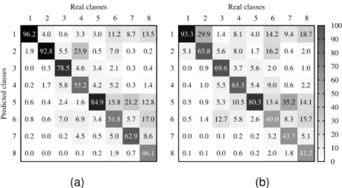
Fig. 2. Confusion matrix of the classification models. (a) PointNet RGB, (b) PointNet. (percent, shade indicates value)
VII. RESULTS
A. Evaluation methodology
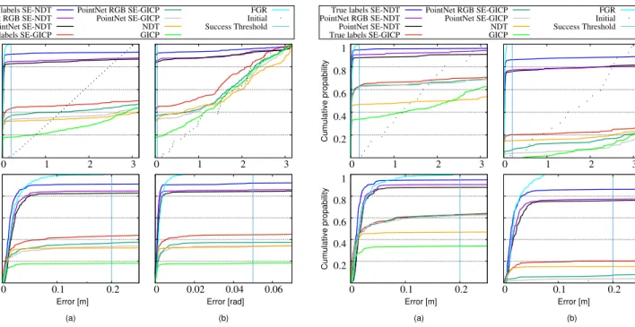
To evaluate the results we use the same methodology as in [20] and [4]. The cumulative distribution function (CDF) plots are interpreted as the probability (vertical axis) that the registration error is lower than the corresponding value on the horizontal axis. The initial perturbations of the data set are also included in Figures 3 and 4, showing the distribution of initial translation error, which could also be interpreted as the performance of a registration method that always returns the identity matrix as the transform. The higher the method’s precision, the closer its curve approaches the vertical axis. The higher the method’s robustness, the larger is the area enclosed between its curve and the initial perturbation curve. To consider a registration successful, both the translation and the rotation error have to be within some limits. We define a registration as successful when the translation error is below0.2m, the rotation error below 0.05rad and when at least one of them is lower than the initial perturbation. We definerobustnessas the percentage of successful registration for the whole dataset, andprecisionas the average translation error on a given percentile of the CDF of errors, so thatP(N) corresponds to the error on the Nth percent.
B. Semantics
The classifier using the RGB model had overall accuracy 86.4 %, while the geometry classifier had79.3 %. Examining the confusion matrices (Figure 2) we notice that the geometry model did not perform as well, especially for natural terrain, hardscape and artifacts (2,6and7). However, consistent mis-classification, e.g. classification of scanning artifacts (7) as buildings (5), should have minimal impact on the registration result, permitting the use of a weaker classifier.
C. Simulated data comparison
The cumulative distributions of translation error for each method are presented in Figure 3a. The top plots cover the entire range of the distribution of the initial error, while the plots on the bottom are zoomed-in to the range of error that a registration is considered successful. We observe that both SE-NDT and SE-GICP outperform their non-semantic versions. This is evident both when classifier or ground truth
Cumulative propability
True labels SE-NDT PointNet RGB SE-NDT PointNet SE-NDT True labels SE-GICP
PointNet RGB SE-GICP PointNet SE-GICP NDT GICP FGR Initial Success Threshold 0.2 0.4 0.6 0.8 1 0 1 2 3 0 1 2 3 (a) Cumulative propability Error [m] 0.2 0.4 0.6 0.8 1 0 0.1 0.2 (b) Error [rad] 0 0.02 0.04 0.06
Fig. 3. Cumulative distributions of registration errors. (a)Translation. (b) Rotation. Top: entire range of initial error. Bottom: zoomed in detail to the range of error considered successful.
labels are used. Fast Global Registration successfully regis-ters all pairs, outperforming in robustness all the methods. The cumulative distribution of orientation error (Figure 3b) follows the same trend.
Table II presents the analytical results of robustness for each algorithm. The first three rows (True, PointNet RGB, PointNet) correspond to the semantic-assisted versions of the algorithms SE-NDT and SE-GICP, while the last row refers to the “standard” D2D-NDT and GICP. The tests show that SE-NDT is over 2 times more robust than SE-GICP. The same holds for SE-GICP and “standard” GICP, while the robustness of “standard” NDT is comparable to SE-GICP.
The precision of the algorithms is compared onP(15), as at this level all methods have successful registrations (GICP fails at P(18)). The results, presented in Table III, indicate that the introduction of semantics improves significantly the precision of both the NDT and GICP versions of the algorithm, with the precision increasing with the accuracy of the semantic labels.
Regarding the execution speed, the reported times are the total CPU time consumed by each method on a single IntelR i7-4700MQ core, although the wall time was 8
times lower due to parallelization. Table IV presents the average execution time for each method. The values in the table do not include the execution time of the classifier. Our implementation classified 200.000 points per second (0.8 second per cloud) on a Nvidia GTX-1080, therefore adding on average1.59 secondsper registration. It should be noted that in real applications, and the KITTI experiments, for each registration only one point cloud goes through the classifier, as the previous one is already classified. In [5] the authors report an execution time of one second for one
Cumulative propability
True labels SE-NDT PointNet RGB SE-NDT PointNet SE-NDT True labels SE-GICP
PointNet RGB SE-GICP PointNet SE-GICP NDT GICP FGR Initial Success Threshold 0.2 0.4 0.6 0.8 1 0 1 2 3 0 1 2 3 (a) Cumulative propability Error [m] 0.2 0.4 0.6 0.8 1 0 0.1 0.2 (b) Error [m] 0 0.1 0.2
Fig. 4. Translation error with different segments of the dataset. (a) Low initial rotation error. (b) High initial rotation error. Top: entire range of initial error. Bottom: zoomed in detail to the range of error considered successful.
million points. Since our method is a lightweight variation of PointNet, using fewer parameters, it can be further optimized to achieve similar performance (0.2 secondper cloud). The increased speed of semantic-assisted GICP can be attributed to the reduced search space for correspondences, as well as convergence before the maximum number of iterations.
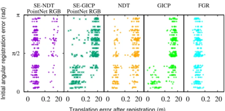
We further examine the performance of the algorithms by comparing the translation error after registration to the initial rotation error. As translation errors above 0.2m are beyond our concern, since they are defined as failed regis-trations, we present this comparison in logarithmic scale in Figure 5. The ideal registration algorithm would have all the points concentrated on a vertical line at0 m. This figure is informative regarding the resilience of the algorithms with regards to the initial rotation error. As expected, Fast Global registration is invariant to the initial error as the initial estimate is not used in the optimization. GICP fails com-pletely when initial rotation error is high, while SE-NDT’s performance is the least affected among the local methods. To further demonstrate this relation, we split the data set into two equal sets according to the initial rotation error. Figure 4a shows the cumulative distribution of translation error after registration for the set with the least50%of initial rotation error. Figure 4b shows the cumulative distribution of translation error after registration for the set with the upper 50% of initial rotation error. We notice a very high discrepancy between the plots on the SE-GICP, GICP and NDT algorithms, while the effect on SE-NDT and FGR is minimal. The difference in the performance of FGR can be attributed to random variation.
0
π/2
π
0 0.2 20
Initial angular registration error (rad)
Translation error after registration (m)
SE-NDT PointNet RGB 0 0.2 20 SE-GICP PointNet RGB 0 0.2 20 NDT 0 0.2 20 GICP 0 0.2 20 FGR
Fig. 5. Translation registration error against initial rotation error.
TABLE II
ROBUSTNESS*OF THE COMPARED METHODS.
Label source SE-NDT SE-GICP FGR
Ground Truth 91 % 44 %
PointNet RGB 85 % 37 %
PointNet 84 % 34 %
No semantics 32 % 18 % 100 %
*Successful in translation and rotation.
tions for SE-NDT showed that there is a trade-off between speed, robustness and precision. For example, if registration speed and robustness are required, in a dataset with high initial errors, the last three (finer) resolutions can be removed, reducing the execution time to0.54 s, with71 %robustness and6.1 cmprecision for the PointNet classifier. Conversely, if the expected initial registration error was low, the first four resolutions could be removed.
We are led to the conclusion that when compared to local registration methods, SE-NDT is more precise and has high invariance to the initial rotation error, approaching the performance of global registration with the advantage of being an order of magnitude faster. For both NDT and GICP, the introduction of semantics reduces the search space for correspondences and the registration is more likely to converge even with high initial error, in sorter time and with higher precision. Furthermore, SE-NDT can be customized, depending on the required application, by picking appropri-ate resolutions.
TABLE III
PRECISION OF THE COMPARED METHODS.
Label source SE-NDT SE-GICP FGR
Ground Truth 0.29 cm 0.31 cm PointNet RGB 0.38 cm 0.60 cm PointNet 0.40 cm 0.62 cm
No semantics 0.74 cm 1.60 cm 0.73 cm Precision at the 15thpercentile of the translation error CDF.
TABLE IV
AVERAGE EXECUTION TIME PER REGISTRATION.
Labels source SE-NDT SE-GICP FGR
Ground Truth 1.63 s 35.96 s
PointNet RGB +1.59 s* 2.33 s 39.52 s PointNet +1.59 s* 2.41 s 39.77 s
No semantics 2.83 s 55.00 s 33.65 s
*Classifier execution time for two clouds.
D. Real data comparison.
We notice that Fast Global Registration exhibits very high accuracy on the first part of the sequence, where the scans are rich in geometric information. However, the performance degrades rapidly when the vehicle enters the motorway, due to the geometric nature of FPFH, and the aliasing of the environment. Figure 7a shows an example of a point cloud with low geometric information, where FGR starts to fail, corresponding to Figure 6a. FGR recovers briefly before the end of the motorway, due to points belonging to buildings.
For the semantic-based algorithms, we removed the points belonging to dynamic classes (vehicles, scanning artifacts). We observed that the classifier had very high false negative rates for those classes, but low false positives, so for every point that belongs to a dynamic class we classify the neigh-bours within a radius of0.5 meteras dynamic. The selection of the radius was based on the approximate scale of a vehicle, and was not fine-tuned. This step is performed to increase the accuracy for this particular class, as we noticed that dynamic objects were the primary cause of registration failure.
SE-NDT was successful in registering the instances where there was low structure, traffic moving parallel to the vehicle, and instances with low semantic information. However, it fails when those conditions are combined. Figure 7b shows an example of a point cloud with low geometric and semantic information, where SE-NDT fails, corresponding to Fig-ure 6b. The version of SE-NDT using edge/surface classifi-cation that we presented in [4] did not fail on those instances as it could capture meaningful semantics on the motorway, but had lower precision at the beginning and ending of the sequence. The edge class was able to capture the vertical poles of the road-side barriers, giving meaningful semantics on those cases. Comparable robustness was noticed for SE-GICP, with the difference that it performed better in cases of low semantics and low geometry (Figure 7b). We can conclude that the performance of SE-NDT is dependent on the ability of the classifier to capture the prominent features of the environment in the direction of geometric aliasing.
VIII. CONCLUSION
In this work we presented a complete pipeline for semantic assisted registration of point clouds. We present two new algorithms, SE-NDT based on the Normal Distributions Transform, and SE-GICP, based on Multichannel General-ized Iterative Closest Point. We used a modified version of PointNet to learn real semantic labels from data, and
Y [m] X [m] SE-NDT SE-GICP GICP NDT FGR Edge SE-NDT Ground truth -800 -400 0 400 0 400 800 1200 1600 (a) (b)
Fig. 6. Path estimated for KITTI sequence 01.
(a)
(b)
Fig. 7. Example of KITTI clouds. (a) Low geometry, (b) Low geometry and low semantics.
test the registration algorithms using the predicted labels on the Semantic3d.net and on the KITTI data set. We demonstrate the ability of SE-NDT to recover from high initial errors, which far exceeds the requirements of mobile robot systems, and at the same time increases precision compared to NDT and GICP. This makes the algorithm applicable to environments with limited structure, where the lack of geometric information can be compensated by the introduction of semantics, given that the classifier captures information relevant to the environment. In future work, we will investigate the use of the PointNet point feature vector before the output layer as input to the semantic registration, instead of the final labels, and test against the probabilistic versions of the algorithms.
REFERENCES
[1] A. Segal, D. Haehnel, and S. Thrun, “Generalized-ICP,” in
Proceed-ings of Robotics: Science and Systems, Seattle, USA, June 2009.
[2] P. Biber and W. Strasser, “The normal distributions transform: a new approach to laser scan matching,” inProc. IEEE/RSJ Int. Conf.
Intelligent Robots and Syst., vol. 3, Oct 2003, pp. 2743–2748.
[3] M. Magnusson, A. Lilienthal, and T. Duckett, “Scan registration for autonomous mining vehicles using 3D-NDT,”J. Field Robotics, vol. 24, no. 10, pp. 803–827, 2007.
[4] A. Zaganidis, M. Magnusson, T. Duckett, and G. Cielniak, “Semantic-assisted 3d normal distributions transform for scan registration in environments with limited structure,” in2017 IEEE/RSJ Int. Conf. on
Intelligent Robots and Syst. IEEE, 2017.
[5] C. R. Qi, H. Su, K. Mo, and L. J. Guibas, “Pointnet: Deep learning on point sets for 3d classification and segmentation,”Proc. Computer
Vision and Pattern Recognition (CVPR), IEEE, vol. 1, no. 2, p. 4,
2017.
[6] T. Hackel, N. Savinov, L. Ladicky, J. D. Wegner, K. Schindler, and M. Pollefeys, “Semantic3d.net: A new large-scale point cloud classification benchmark,”ISPRS Annals of Photogrammetry, Remote
Sensing and Spatial Information Sciences, vol. IV-1/W1, 04 2017.
[7] Q.-Y. Zhou, J. Park, and V. Koltun, “Fast global registration,” in
European Conference on Computer Vision. Springer, 2016, pp. 766–
782.
[8] A. Geiger, P. Lenz, and R. Urtasun, “Are we ready for autonomous driving? the KITTI vision benchmark suite,” in Proc. IEEE Conf.
Comput. Vision and Pattern Recognition, 2012, pp. 3354–3361.
[9] P. Besl and N. McKay, “A Method for Registration of 3-D Shapes,”
IEEE Trans. on Pattern Analysis and Machine Intell., vol. 14, no. 2,
pp. 239–256, Feb 1992.
[10] G. Agamennoni, S. Fontana, R. Y. Siegwart, and D. G. Sorrenti, “Point clouds registration with probabilistic data association,” in2016 IEEE/RSJ International Conference on Intelligent Robots and Systems
(IROS), Oct 2016, pp. 4092–4098.
[11] A. N¨uchter, O. Wulf, K. Lingemann, J. Hertzberg, B. Wagner, and H. Surmann, “3D mapping with semantic knowledge,” inRobot Soccer
World Cup. Springer, 2005, pp. 335–346.
[12] R. B. Rusu, N. Blodow, and M. Beetz, “Fast point feature histograms (FPFH) for 3d registration,” in2009 IEEE Int. Conf. on Robotics and
Automation, May 2009, pp. 3212–3217.
[13] T. Stoyanov, M. Magnusson, and A. J. Lilienthal, “Point set registra-tion through minimizaregistra-tion of the L2 distance between 3D-NDT mod-els,” inProc. IEEE Int. Conf. Robotics and Automation, Minnesota, USA, 2012, pp. 5196–5201.
[14] B. Huhle, M. Magnusson, W. Strasser, and A. J. Lilienthal, “Regis-tration of colored 3D point clouds with a Kernel-based extension to the normal distributions transform,” inProc. IEEE Int. Conf. Robotics
and Automation, May 2008, pp. 4025–4030.
[15] J. Servos and S. L. Waslander, “Using RGB information to improve NDT distribution generation and registration convergence,” in
Pro-ceedings of Int. Conf. on Intelligent Unmanned Syst., vol. 10, 2014.
[16] T. Schmiedel, E. Einhorn, and H. M. Gross, “IRON: A fast interest point descriptor for robust NDT-map matching and its application to robot localization,” inProc. IEEE/RSJ Int. Conf. Intelligent Robots
and Syst., Sept 2015, pp. 3144–3151.
[17] Y. Chen and G. Medioni, “Object modeling by registration of multiple range images,” in Proc. IEEE Int. Conf. Robotics and Automation, vol. 3, Apr 1991, pp. 2724–2729.
[18] M. Magnusson, N. Vaskevicius, T. Stoyanov, K. Pathak, and A. Birk, “Beyond points: Evaluating recent 3D scan-matching algorithms,” in
Proc. IEEE Int. Conf. Robotics and Automation, 2015, pp. 3631–3637.
[19] J. Servos and S. L. Waslander, “Multi channel generalized-icp,” in 2014 IEEE International Conference on Robotics and Automation
(ICRA), May 2014, pp. 3644–3649.
[20] F. Pomerleau, F. Colas, R. Siegwart, and S. Magnenat, “Comparing ICP variants on real-world data sets: Open-source library and exper-imental protocol,”Autonomous Robots, vol. 34, no. 3, pp. 133–148, 2013.