UC Berkeley
UC Berkeley Electronic Theses and Dissertations
Title
Learning to Generalize via Self-Supervised Prediction Permalink https://escholarship.org/uc/item/01p3020h Author Pathak, Deepak Publication Date 2019 Peer reviewed|Thesis/dissertation
eScholarship.org Powered by the California Digital Library University of California
by Deepak Pathak
A dissertation submitted in partial satisfaction of the requirements for the degree of
Doctor of Philosophy in Computer Science in the Graduate Division of the
University of California, Berkeley
Committee in charge: Professor Trevor Darrell, Chair Professor Alexei A. Efros, Chair
Professor Jitendra Malik Professor Alison Gopnik
Learning to Generalize via Self-Supervised Prediction
Copyright 2019 by Deepak Pathak
Abstract
Learning to Generalize via Self-Supervised Prediction by
Deepak Pathak
Doctor of Philosophy in Computer Science University of California, Berkeley
Professor Trevor Darrell, Chair Professor Alexei A. Efros, Chair
Generalization, i.e., the ability to adapt to novel scenarios, is the hallmark of human intelligence. While we have systems that excel at recognizing objects, cleaning floors, playing complex games and occasionally beating humans, they are incredibly specific in that they only perform the tasks they are trained for and are miserable at generalization. Could optimizing towards fixed external goals be hindering the generalization instead of aiding it? In this thesis, we present our initial efforts toward endowing artificial agents with a human-like ability to generalize in diverse scenarios. The main insight is to first allow the agent to learn general-purpose skills in a completely self-directed manner, without optimizing for any external goal.
To be able to learn on its own, the claim is that an artificial agent must be embodied in the world, develop an understanding of its sensory input (e.g., image stream) and simultaneously learn to map this understanding to its motor outputs (e.g., torques) in anunsupervised manner. All these considerations lead to two fundamental questions: how to learn rich representations of the world similar to what humans learn?; and how to re-use such a representation of past knowledge to incrementally adapt and learn more about the world similar tohow humans do? We believe prediction is the key to this answer. We propose generic mechanisms that employ prediction as a self-supervisory signal in allowing the agents to learn sensory representations as well as motor control. These two abilities equip an embodied agent with a basic set of general-purpose skills which are then later repurposed to perform complex tasks.
We discuss how this framework can be instantiated to develop curiosity-driven agents (virtual as well as real) that can learn to play games, learn to walk, and learn to perform real-world object manipulation without any rewards or supervision. These self-directed robotic agents, after exploring the environment, can generalize to find their way in office environments, tie knots using rope, rearrange object configuration, and compose their skills in a modular fashion.
i
Contents
List of Figures vi
List of Tables viii
Acknowledgments ix
1 Introduction 1
1.1 Background . . . 1
1.2 Current Dominant Paradigms for Generalization . . . 3
1.2.1 Generalization by Data . . . 3
1.2.2 Generalization by Regularization/Design . . . 3
1.2.3 Generalization by Meta/Transfer Learning . . . 4
1.2.4 Generalization by Domain Adaptation . . . 4
1.2.5 Generalization by End-to-End Reinforcement . . . 4
1.3 Proposed Solution . . . 5
1.3.1 Learning to Generalize via Self-Supervised Prediction . . . 6
I
Self-Supervised Representation Learning
8
2 Learning Representation via Context Prediction 9 2.1 Context encoders for image generation . . . 112.1.1 Encoder-decoder pipeline . . . 11 2.1.2 Loss function . . . 13 2.2 Implementation details . . . 15 2.3 Evaluation . . . 16 2.3.1 Semantic Inpainting . . . 17 2.3.2 Feature Learning . . . 17 2.4 Related work . . . 19
3 Discovering Objects by Observation and Interaction 22 3.1 Evaluating Feature Representations . . . 24
iii
3.2.1 Training a ConvNet to Segment Objects . . . 25
3.2.2 Experiments . . . 25
3.3 Learning Features by Watching Objects Move . . . 28
3.3.1 Unsupervised Motion Segmentation . . . 28
3.3.2 Learning to Segment from Noisy Labels . . . 29
3.4 Evaluating the Learned Representation . . . 31
3.4.1 Transfer to Object Detection . . . 31
3.4.2 Low-shot Transfer . . . 33
3.4.3 Impact of Amount of Training Data . . . 33
3.4.4 Transfer to Other Tasks . . . 33
3.5 Object-centric Representation via Interaction . . . 34
3.5.1 Experimental Setup . . . 36
3.5.2 Instance Segmentation by Interaction . . . 37
3.5.3 Results and Evaluations . . . 38
3.6 Related Work . . . 39
3.7 Discussion . . . 40
II
Learning to Act via Self-Supervised Exploration
41
4 Curiosity-driven Exploration by Self-supervised Prediction 42 4.1 Curiosity-Driven Exploration . . . 454.1.1 Prediction error as curiosity reward . . . 46
4.1.2 Self-supervised prediction for exploration . . . 46
4.2 Experiments . . . 48
4.2.1 Experimental Setup . . . 48
4.2.2 Sparse Extrinsic Reward Setting . . . 49
4.2.3 No Reward Setting . . . 51
4.2.4 Generalization to Novel Scenarios . . . 52
4.3 Large-Scale Study of Curiosity-Driven Learning . . . 54
4.3.1 Feature spaces for forward dynamics . . . 55
4.3.2 Practical considerations in training with only curiosity . . . 57
4.3.3 ‘Death is not the end’: infinite horizon . . . 58
4.4 Large-Scale Experiments . . . 58
4.4.1 Curiosity-driven learning without extrinsic rewards . . . 58
4.4.2 Generalization across novel levels in Super Mario Bros. . . 62
4.4.3 Curiosity with Sparse External Reward . . . 63
4.5 Related Work . . . 64
4.6 Discussion . . . 66
5 Self-Supervised Exploration via Disagreement 68 5.1 Exploration via Disagreement . . . 70
5.1.1 Disagreement as Intrinsic Reward . . . 70
5.1.2 Exploration in Stochastic Environments . . . 71
5.1.3 Differentiable Exploration for Policy Optimization . . . 72
5.2 Implementation Details and Baselines . . . 73
5.3 Experiments . . . 74
5.3.1 Sanity Check in Non-Stochastic Environments . . . 74
5.3.2 Exploration in Stochastic Environments . . . 75
5.3.3 Differentiable Exploration in Structured Envs . . . 76
5.4 Discussion . . . 79
III
From Skills to Goal-Directed Expertise
80
6 Zero-Shot Visual Imitation 81 6.1 Learning to Imitate without Expert Supervision . . . 836.1.1 Learning the Goal-conditioned Skill Policy (GSP) . . . 84
6.1.2 Forward Consistency Loss . . . 84
6.1.3 Goal Recognizer . . . 86
6.2 Experiments . . . 88
6.2.1 Rope Manipulation . . . 89
6.2.2 Navigation in Indoor Office Environments . . . 90
6.2.3 3D Navigation in VizDoom . . . 92
6.3 Related Work . . . 93
6.4 Discussion . . . 95
IV
Generalization via Modularity
96
7 Learning to Control Modular Self-Assembling Morphologies 97 7.1 Environment and Agents . . . 987.2 Learning to Control Self-Assemblies . . . 100
7.2.1 Co-evolution: Linking/Unlinking as an Action . . . 101
7.2.2 Modularity: Self-Assembly as a Graph of Limbs . . . 101
7.2.3 Dynamic Graph Networks (DGN) . . . 102
7.3 Experiments . . . 103
7.3.1 Learning to Self-Assemble . . . 104
7.3.2 Zero-Shot Generalization to Number of Limbs . . . 106
7.3.3 Zero-Shot Generalization to Novel Environments . . . 106
7.4 Related Work . . . 107
7.5 Discussion . . . 108
v
A Experimental Details for Curiosity-driven Exploration 111
A.1 Implementation Details . . . 111 A.2 Additional Results . . . 112
B Experimental Details for Zero-Shot Imitation 114
B.1 Rope Manipuation . . . 114 B.2 Navigation in Indoor Office Environments . . . 114 B.3 3D Navigation in VizDoom . . . 115
C Experimental Details for Dynamic Graph Networks 117
C.1 Implementation and Training details . . . 117 C.2 Fixed-Graph Baseline vs. Number of Limbs . . . 117 C.3 Pseudo Code for DGN Algorithm . . . 118
List of Figures
1.1 Generalization of ImageNet trained model to YouTube video frames . . . 2
2.1 Qualitative illustration of context prediction task . . . 10
2.2 The architecutre of Context Encoder . . . 11
2.3 Semantic inpainting results for context encoder . . . 12
2.4 Inpainting regions for context prediction . . . 14
2.5 Comparison with content-aware fill (photoshop) . . . 15
2.6 Semantic inpainting using different methods . . . 16
2.7 Arbitrary region inpainting via context encoder . . . 17
2.8 Nearest Neighbors in Context Encoder feature space . . . 18
3.1 Motion-based grouping as supervisory signal . . . 23
3.2 Overview of learning features by watching objects move . . . 24
3.3 Representation trained on manually-annotated segments from COCO . . . 26
3.4 Variation of VOC object detection accuracy wrt noise . . . 26
3.5 Degraded masks to measure the impact of learned segmentation quality . . . 27
3.6 Our model learns from as well as refines the noisy training data . . . 28
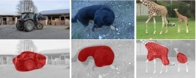
3.7 Examples of segmentations produced by our model on held out images . . . 30
3.8 Variation of representation quality with amount of data . . . 32
3.9 Results on classification and segmentation tasks . . . 33
3.10 Overview of learning segmentation by interaction . . . 35
3.11 Quantitative evaluation of the segmentation model on the held-out set . . . 37
4.1 Discovering how to play Super Mario Bros without rewards . . . 43
4.2 Overview of Intrinsic Curiosity Module . . . 45
4.3 Samples from VizDoom 3-D environment . . . 48
4.4 Quantitative results of curiosity-driven exploration on VizDoom . . . 49
4.5 Robustness of ICM to uncontrollable distractors . . . 50
4.6 Reward-free exploration in VizDoom . . . 52
4.7 Generalization evaluation of pre-trained curiosity agent . . . 54
4.8 Snapshot of the 54 environments investigated . . . 55
vii
4.10 Large-scale comparisons on Mario and Pong . . . 61
4.11 Mario generalization experiments . . . 63
4.12 Unity 3D navigation experiments . . . 63
4.13 Noisy TV with remote experiment in Unity . . . 67
5.1 Self-Supervised Exploration via Disagreement . . . 69
5.2 Sanity Check in Non-Stochastic Environments . . . 74
5.3 Toy example to show usefulness of disagreement . . . 76
5.4 3D Navigation in Unity . . . 76
5.5 Stochastic Atari Games . . . 77
5.6 Disagreement-based exploration with or without the differentiability . . . 77
5.7 Object interaction rate wrt the number of samples . . . 78
6.1 Different architecture for goal-conditioned policy . . . 82
6.2 Qualitative visualization of rope manipulation results . . . 87
6.3 Quantitative results for rope manipulation . . . 88
6.4 Visualization of the TurtleBot navigation trajectory . . . 89
6.5 Trajectory of TurtleBot following a multi-step demonstration . . . 91
7.1 Learning to control self-assemblies via dynamic graph networks . . . 98
7.2 Illustration of locomotion and standing up enviroments . . . 99
7.3 Co-evolution of morphology w/ control during training . . . 102
7.4 Learning plots for self-assembling agents . . . 104
8.1 Deploying curiosity on a custom designed low-cost arm . . . 110
A.1 Pure curiosity-driven exploration in Atari . . . 113
List of Tables
2.1 Semantic inpainting accuracy for Paris StreetView dataset . . . 16
2.2 Quantitative comparison of representation learning methods . . . 19
3.1 Object detection on VOC’12 with various pretrained ConvNets . . . 31
3.2 Quantitative comparison of segmentation by interaction with baselines . . . 38
4.1 Quantitative evaluation in Super Mario Bros. . . 53
4.2 Categorization of different feature spaces considered . . . 56
6.1 Quantitative evaluation of various methods for navigation . . . 90
6.2 Quantitative evaluation of TurtleBot’s performance in multi-step case . . . 92
6.3 Quantitative evaluation in VizDoom . . . 94
7.1 Zero-Shot generalization to number of limbs . . . 105
7.2 Zero-Shot generalization to novel environments . . . 105
A.1 Curiosity with extrinsic reward in Atari . . . 113
B.1 Detailed quantitative evaluation of TurtleBot for maze and loop tasks . . . 115
ix
Acknowledgments
It just so happens that I have to take credit as the sole author of this dissertation. In reality, this is a purely collaborative effort, from working alongside my advisors, mentors, colleagues, friends, and family. A number of people have continually supported and guided me, throughout my Ph.D., which in turn has made this dissertation a reality.
I would like to start off by expressing sincere gratitude to my dear Ph.D. advisors, Trevor Darrell, and Alyosha Efros, for taking me in as their advisee. Ever since my admissions interview with Trevor, I was certain that I wanted to join his research group, and feel grateful for the opportunity to have been a part of it. Trevor shielded me from any external hiccups and allowed me to primarily focus on research. No matter what the issue was, I could always count on him to help me find a way out of it. One of the biggest strengths Trevor has instilled in me is to not give up. Many of my paper submissions would not have been possible if he did not consistently have my back, always helping and encouraging. Trevor also taught me how to collect my ever wandering thoughts into a potentially cool idea. Despite being responsible for leading such a large research group, Trevor has this unique ability to take extremely good care of each of his students. I am thankful for his continued support and guidance as I embark on my academic journey ahead.
As I officially graduate and the time to leave UC Berkeley comes closer, I wonder if Alyosha’s imprint on me will ever leave me. I hope it does not. In his own words, I carry a good discriminator model in my mind. His guidance and thinking style has imprinted on me forever. I used to be an engineer, but it is because of Alyosha that I can (even remotely) now consider myself a scientist in disguise. Looking at the big picture, constantly questioning fundamentals, how to write in a concise and punchy manner, being selfless in every circumstance, being bold yet reasonable, and thinking long-term, are some of the invaluable gems I received by working with him. I owe it to him, for showing me the Science in Computer Science. I was and still, am fascinated by the stories of how huge scientific discoveries were made. I use to think that the era was over, but Alyosha gave me hope that maybe it has not. From long late-night discussions, to even longer arguments during hikes, I think I have spent way more personal hours with my advisor than any other Ph.D. student in the current era. Of course, we were not as productive in the short term, but I know it helped me gather knowledge, which will someday, in turn, help me become a scientist! I could go on and on and fill pages had I begun writing this in time, but again, “if you do it at the last minute, it only takes a minute” – something I wish I can unlearn!
I am also extremely grateful to have Jitendra Malik and Alison Gopnik as my thesis committee members. The ideology proposed in this dissertation is heavily motivated by their research principles. I learned from Jitendra about the importance of scientific rigor, pursuing big ideas and being well-read. He is a walking encyclopedia, and the gold standard for all of us to aim for. Much of my memories of the UC Berkeley culture revolve around the trio of Jitendra, Trevor, and Alyosha, participating actively in Monday morning reading groups.
I would like to also thank Pieter Abbeel and Sergey Levine for their precise critique of my ideas. My maneuvering into the Reinforcement Learning (RL) world would not have been possible without them. I would like to especially thank Pieter for helping with my faculty applications and taking the time out for frequent meetings to discuss research ideas.
Working with Abhinav Gupta at Pittsburgh was one of the best times in my Ph.D. I learned a lot from him, about research and mentoring students, in those few months. His research style has had a great impact on me. I am excited about having him as my colleague and mentor at CMU.
I have also been greatly influenced by the research journeys of Yann Lecun and Geoff Hinton as they helped make deep learning what it is today. Having been fortunate enough to meet with Yann in person when I was in my first year of Ph.D., I was amazed by his humility. The few discussions I have had with him over the years have acted as great motivation for me to aspire to do great research. I am also thankful to Miro Dud´ık with whom I interned at Microsoft Research (MSR), New York, during my third year of undergraduate studies. If I had not met him, I would have never applied for a Ph.D. program. I also thank Vinay Namboodiri for being a great mentor.
I am extremely lucky to have also worked with Philipp Krhenbhl. Thank you for teaching me optimization, how to think concretely about research ideas, trusting intuitions, being confident, and the importance of being mathematically rigorous. My internship with Ross Girshick, Bharath Hariharan and Piotr Doll´ar further inculcated in me the extreme value of rigorous experimentation and not discarding any hypothesis without concrete evidence. I also had a great time collaborating with Phillip Isola on our crazy, over a year-long project – during which I learned a lot from him.
I would like to also thank Pulkit Agrawal - who grew from being my academic senior to a great friend over the years. We did many projects together, and brainstormed some of the coolest ideas – some made it in writing and some eventually will. I am thankful for his help on numerous accounts, including my job talk preparation. However, the biggest thing that I owe him for is a piece of valuable advice he gave me once - to listen to and get feedback from everyone but decide on your own. He taught me how not to get discouraged by criticism.
My memories of SDH7 will not be complete without Judy Hoffman, Ning Zhang, Jeff Donahue, Jon Long, Evan Shelhamer, Lisa Hendricks, Eric Tzeng, and Samaneh Azadi. Evan has this unique ability to come up with the most amazing titles and brewing the strongest coffee – two things I have bugged him a lot for – thanks for bearing with me! I am also thankful to Jun-Yan and Richard for being great friends and peers. Futile attempts at continuing to go to the gym with Jun-Yan, Richard and Tae are one of the most comical memories of my graduate life. Jun-Yan and I used to often stay until quite late in the lab and
xi
I thank him for dropping me home several times. We have spent countless hours discussing research and brainstorming several other not-so-important topics. I am really excited to have him as my colleague at CMU. I thank Shubham for always helping me debug my ideas and showing me corner cases which I would have missed otherwise. Thanks to Saurabh for being a great academic senior and entertaining my endless research questions. Thanks to Somil for teaching me controls.
Special thank you to all the postdocs - Jiashi Feng, Marcus Rohrbach, Sergio Guadarrama, Anja Rohrbach, Jo˜ao Carreira, Andrew Owens, Dinesh Jayaraman, Angjoo Kanazawa, and David Fouhey. Thank you, David, for adding humor to our lab and Angjoo for preventing the labs from being awfully quiet.
My time at UC Berkeley would not have been the same without my awesome academic and research peers. I feel privileged that I overlapped with one of the most amazing student cohorts at UC Berkeley. I am extremely thankful to Carl Doersch, Shiry Ginosar, Tinghui Zhou, Yang Gao, Taesung Park, Dequan Wang, Alan Jabri, Ashish Kumar, Eliza Kosoy, Rachit Dubey, Coline Devin, Ronghang Hu, Huazhe Xu, Jasmine, Sasha, Erin Grant, Avi Singh, Chelsea Finn, Vitchy Pong and Kelvin Xu.
Finally, I would like to thank the amazing masters and undergraduate students whom I was fortunate to work with. I especially thank Parsa for being patient with me all these years. I am very lucky to have worked with Chris, Fred, Dian, Michael, Dhiraj, Pratyusha and WenXuan.
Hanging out with Abhishek, Somil, Shubham, Tejas, Varun, and Vivek has often helped me not to get homesick. 1735 Cedar St. has been my defacto mailing address at Berkeley. I would like to also thank Weicheng Kuo and Ke Li - my first friends at UC Berkeley. My first few years would not have been so much fun if it did not involve attending classes, working on assignments, and having lunch with them – a very special mention to them for agreeing to countless visits to Urban Turban!
I am extremely grateful to Nikita for being on my side, keeping me sane and for being my core strength all these years – thank you for entertaining my numerous last-minute requests for proofreading! I would also like to thank my sister Divya for her love, support and for keeping me attached to the home. Finally, I would like to thank my parents Durga Pathak and Madhwa Nand Pathak. I would not have been fortunate enough to be the first engineer and first doctorate in our entire family tree had it not been for their support. I wonder if I can ever match the hard work they put in to provide myself and Divya with the opportunities that have made us reach where we are today. I am always humbled by remembering the roots of their journey. I sincerely believe that they made progress worthy of two generations in one, by allowing me to match shoulders with the most modern and developed society. I dedicate this thesis to them for their uncountable sacrifices, boundless support, and unconditional love.
Thanks to Facebook, Nvidia, and Snapchat for awarding me their graduate fellowships and supporting my research.
Chapter 1
Introduction
Consider an American college student embarking on her first trip abroad. She lands in Paris and, incredibly, she can still navigate the streets of this new city, spot cars and traffic signs, enter stores, etc., even though all of those look quite different in France than in the States. We as humans are naturally able to re-use our past experiences to adapt to novel scenarios. This ability to generalize makes us who we are. Generalization is the hallmark of human intelligence. While we have algorithms that excel at learning to translate languages, play complex games and even beat humans at it, they are miserable at generalization. For instance, a classification model that achieves super-human performance on the famous ImageNet dataset fails dramatically when deployed on a wearable camera in the real world. A robot that is an expert in the intricate task of putting a car engine together will fail at an apparently ‘simple’ task of putting plates into a dishwasher. Indeed, as noted by Moravec: the hard things are easy, and the easy things are hard.
1.1
Background
Since the inception of early ideas proposed by Alan Turing 70 years ago [246], AI has come a long way in building expert specialist systems. We have systems that can master the complex game of Go [226], classify images [95,128], find objects in them [94], recognize speech [89], generate audio [168], translate languages [265], play table tennis [157] and perform many mundane industrial tasks. However, in contrast to humans, our current machine learning algorithms are incredibly narrow in performing the tasks they are trained for. A system that is champion in Go cannot translate languages. Needless to say, our current systems are missing the common-sense possessed by humans. However, the problem is more fundamental and rooted in the way we approach artificial intelligence.
Consider the following case study. Classification challenge on ImageNet [205] has led to the development of the methods that can classify images with superhuman accuracy (over 85%). This has been the flagship benchmark result and a crown jewel in the success of deep neural networks. However, these models completely fail to generalize when tested on
CHAPTER 1. INTRODUCTION 2
Figure 1.1: Sample outputs of ResNet-50 model trained on ImageNet when tested on frames of a video from YouTube. Left are representative samples of Labrador class from ImageNet, and right are the examples of false predictions generated by the model on video frames.
real-world videos, and the accuracy dramatically falls to less than one third than that in ImageNet. As shown in Figure 1.1, one such model, ResNet-50 [95], misclassifies Labrador as detects classes like Ray (fish), Cobra (snake) and Flatworm (also see [204] for examples). Why is that the case? ImageNet contains images that have objects at the center of the image, taken from a good angle with photographer bias – the conditions which do not prevail in the general videos and have arbitrary changes in pose, motion blur, etc.
The reason is rather unsurprising, but questions a fundamental assumption in machine learning. Most of the ML approaches assume that the distribution at test time will be the same as seen during training. This could be true for passively collected datasets or simulated environments, but it does not hold in the real world. We cannot hope to capture all the possibilities, which one could ever encounter in the future, in a training dataset collected once ahead of time.
Interestingly, this issue is not specific to recent approaches, it rather dates back to the inception of AI. As the story goes, ARPA (now called DARPA) organized a challenge for classifying the presence of a tank in images in the early 1960s. They released a dataset of images with and without tanks. AI researchers at the time trained the classifiers (perhaps Perceptron) and achieved high accuracy on the dataset. However, the models failed to generalize to the tanks in the real world. It turns out that the non-tank images in the dataset were of forests in cloudy days, and tank images were captured in sunny days. Thus, instead of understanding tanks, the model found a shortcut by simplifying thresholding brightness intensities. Whether apocryphal or not 1, this cautionary tale very accurately captures a problem that is still unsolved by all means.
1The oldest reference we could find is Kanal and Randall, 1964 [115]. Although, the true version of this
1.2
Current Dominant Paradigms for Generalization
One of the reasons for assuming the train and test distribution be same is that it is easy to handle mathematically. In contrast, the scenarios with changing the task or data distribution are difficult to define precisely. Indeed, if the new data or tasks the model is supposed to generalize to are too far from the training ones, there might not be any overlap of reusable knowledge to generalize. It has to be rather a smooth continuum of changing distribution where this notion of similar enough is really hard to capture mathematically. To scale our AI systems beyond the lab environments to real-world setups, our models must learn to generalize across changing data as well as task distributions. There have been several ways to try to address this challenge, however, they all have come up short as we discuss below:1.2.1
Generalization by Data
One way to force generalization is to use lots of data. The hope is that, given huge labeled data, the model would have seen almost all possibilities such that generalization at test time reduces to just an interpolation problem. To concretize it, consider that we would like to train a function f(x) that takes an input xand outputs label y from datasetDtrain = {x, y}.
The argument is that as |Dtrain| →inf, generalization would become trivial. This is of course
practically impossible to do for all possible tasks, however, it is worth analyzing scientifically. For instance, in our tank example, it would mean that we need to collect images of tanks in rainy days, cloudy days, and all possible scenarios. Would that be enough? Unlikely because our world is continuously changing, and by the time we are done recording the current snapshots, the model of a tank would have changed. Hence, just scaling data and compute is implausible as a solution to building agents that can function in our ever-changing, real, complex world.
1.2.2
Generalization by Regularization/Design
One of the major reasons for failure to generalize is that the model ends up overfitting to spurious correlations instead of desired properties. The high-level goal in this paradigm is to restrict the space of possible instantiations of our function f such that unwanted correlations are avoided by construction. Classic approaches like L2/L1/elastic-regularizations [91] apply broadly to almost all statistical methods. The less obvious ones are the constraints that one could use by exploiting the domain structure. For instance, the structure of convolution has been immensely successful in neural networks for dealing with raw images [134]. Other examples include residual connections for training bigger networks [95], modularity in learned components to incorporate structure in language and images, etc. [8] etc. However, these constraints or structure help by reducing the probability of spurious correlations, but not enough. In our tank classification example, these design choices will help with overfitting but still won’t be able to avoid the shortcut of modeling brightness.
CHAPTER 1. INTRODUCTION 4
1.2.3
Generalization by Meta/Transfer Learning
Instead of training the models to optimize for low error rate on the training set, one could directly optimize for generalization to unseen examples. The idea is captured by the family of algorithms called meta learning [18,160,214,244] or transfer learning [33]. The standard approach of optimizing for best performance on the training set is rephrased to optimizing for a solution on training set such that it achieves good performance on some held-out data. Hence, instead of training on a single fixed training set, the models are trained on a family of tasks to generalize from one to another (see [65] for a detailed discussion). This paradigm is certainly optimizing for the correct behavior and perhaps the model will learn less spurious features. However, it still relies on a large amount of supervised labeled examples in the meta-training phase. More importantly, to optimize transfer across tasks/dataset directly, the tasks/datasets in the family has to be closely tied in practice. In such a case, the main challenge again reduces to the original core problem, i.e., how to generalize beyond the (close) family of tasks/datasets seen during training.
1.2.4
Generalization by Domain Adaptation
Domain adaption follows an alternative approach to generalizing the learned model to test distribution. The idea is to rather transform the data at test time such that its distribution becomes similar to training [27,43,96,207]. The most common approach is to transform the data such that discrepancy is minimized between training and test data without explicitly requiring labels for test examples (see [101] for discussion). For instance, in the tank classification case, one could transform the tank images from rainy days, cloudy days, etc. to look like a tank in sunny days by employing some perceptual losses on the images. However, this exposes a critical issue that this transformation has to be learned for every new scenario encountered by the agent in the future because the model still simply classifies brightness and does not understand what a tank is. This is so because this paradigm sidesteps the core problem of learning understanding the true structure to generalize.
1.2.5
Generalization by End-to-End Reinforcement
End-to-end learning from scratch is one of the most popular paradigms in machine learning today. Instead of solving intermediate tasks in stages, the agent could directly solve for the end goal and learn necessary abstractions without much specific domain knowledge. A generic family of algorithms called reinforcement learning (RL) [241] encapsulate this approach. RL has emerged as a popular method for training agents to perform complex sensorimotor tasks. In RL, the agent’s policy is trained by maximizing a reward function that is designed to align with the task. However, designing a well-shaped reward function is a notoriously challenging engineering problem, and such rewards are often absent in the real world. Hence, in practice, most of the success in RL has been achieved where this dense and well-shaped reward is easily available, e.g., a running ‘score’ in video games [155], or zero-sum games like chess or
Go [226]. Moreover, rewards are very specific to the task and environment that they are defined for, thus, generalizing to new tasks/scenarios is a serious concern in RL [98].
1.3
Proposed Solution
The ability to generalize to novel, changing scenarios is essential for artificial agents to function in real and diverse environments. As discussed above, the current dominant paradigm of supervised learning, which relies on training with human-labeled examples, is unlikely to achieve this goal. Having a human provide lots of labels for every possible task that an agent could ever encounter is like building a ladder to the moon — there might never be enough labels! Indeed, supervised learning is not how most learning transpires in ecological contexts. Instead, all that is available to a biological agent is just raw sensory data and the ability to act in the world to collect more data. More importantly, it could be that the mere presence of a fixed goal (conveyed by human-labeled examples or rewards) tempts our algorithms to cheat by modeling spurious correlations.
What if we remove this extrinsic goal? In the absence of a goal, our agent can no longer ‘cheat’ as there would be nothing to find a ‘shortcut’ for. This is not as strange as it sounds.
Developmental psychologists talk about intrinsic motivation (i.e., curiosity) as the primary driver in the early stages of development [83,206,230]: babies appear to employ (extrinsic) goal-free exploration to learn skills that will be useful later on in life, for instance, throwing, pushing objects and interacting with the world in seemingly random ways. In fact, this form of learning is not specific to humans. The example, given by Alison Gopnik [82], of the contrast between domestic chicken and New Caledonian crow, precisely illustrates the crucial role of such intrinsic exploration phase in shaping the intelligence of species. Domestic chicken (also, ducks, geese, and turkeys) are often considered as the dumbest of all birds. They are very good at the task of pecking grains, but pretty much useless otherwise. In contrast, a New Caledonian crow is one of the intelligent bird species, and can even figure out the use of a tool by shaping hooks to retrieve food [256]. Despite having similar cortical structure, chickens are specialists while these crows are impressive generalists. Gopnik argues that it is connected to the length of their childhood period of exploration without any end-goals. While chickens become mature and functional in just a few months, the baby New Caledonian crows depend on their caretaker to feed and nurture them up to 2 years, which is a long time in the lifespan of a bird. This link between long childhood and intelligence of a species has been studied in depth by Piantadosi and Kidd, 2016 (see Figure 3 in [189]). Across several primate species, the length of the weaning period seemed to be strongly correlated with how intelligent the species is. One crucial aspect of this seemingly frivolous ‘play’ is that it allows these biological agents to learn how to continually adapt and increase knowledge about the world without any explicit supervision or extrinsic end-goal.
CHAPTER 1. INTRODUCTION 6
1.3.1
Learning to Generalize via Self-Supervised Prediction
In this dissertation, inspired by these prominent ideas, we propose initial directions towards the grand question of building artificial agents that learn, act and display seamless general-purpose behavior. Our key emphasis is on building agents that continually develop knowledge and acquire skills just from their own collected data by usingdata as its own supervision. We begin with minimal assumptions and build complete systems that learn from raw sensory data. To be able to learn from scratch, the claim is that an artificial agent must be embodied in the world, develop an understanding of its sensory input (e.g., image stream) and simultaneously learn to map this understanding to its motor outputs (e.g., torques) in an unsupervised
manner.
All these considerations lead to two fundamental questions: how to learn rich representa-tions of the world similar to what humans learn?; and how to re-use such a representation of past knowledge to incrementally adapt and learn more about the world similar to how
humans do? We believe prediction is the key to this answer. We propose generic mechanisms that employ prediction as a self-supervisory signal in allowing the agents to learn sensory representations as well as act on these representations to govern motor control. These two abilities should equip an embodied agent with a basic set of general-purpose skills. Later, these skills can be stitched together to achieve end-goals or tasks given to the agent, by planning using the learned models with little to no supervision from outside. This thesis outlines this ideology in detail and concretizes these ideas into algorithms which are demonstrated via several case studies, ranging from passive datasets, games to real robotics setups, as summarized below.
I. Self-Supervised Representation Learning Our world is diverse, yet highly struc-tured, and humans have an uncanny ability to make sense of it. This ability to build rich representations of raw sensory data is indispensable for agents learning to operate on their own. But how is this structure discovered in the first place? In Part I, we propose two approaches to learn sensory representations. Chapter 2 proposes Context Encoders which employ prediction of context as supervision to learn visual features. Then in Chapter 3, we extend this ideology to learn representation by leveraging the Gestalt principle of common-fate [257], i.e., pixels that move together tend to belong together, which explicitly guides the perception of object boundaries. These groupings are either obtained by watching passive videos, or by active interaction of a robot.
II. Learning to Act via Self-Supervised Exploration Learning to see the world the way we do is only the first step in building a self-supervised autonomous agent. An agent will be able to adapt and acquire increasingly complex behaviors only when it learns to use its sensory representation to act. However, acting in the world is unlike passive observations because the data is sequentially dependent on the past which leads to exponentially many possible trajectories and makes it intractable to figure out the ones that constitute useful skills. In Chapter 4, we leverage self-supervised prediction to formulate a notion ofcuriosity
in artificial agents that allows learning to act without any extrinsic supervision or rewards. Chapter 5 extends this formulation into an explicitly differentiable objective such that it can be efficiently scaled to real robots.
III. From Skills to Goal-Directed Expertise Parts I and II discuss how an agent could acquire sensorimotor skills of increasing complexity with no knowledge of labels or tasks. However, to be useful for real-world tasks, the agent will eventually have to develop the ability to perform a specific task given to it. One way is to finetune a pre-trained self-supervised agent with task-specific rewards. However, reward-based finetuning is inefficient and not scalable to real robots. In Chapter 6, we follow an alternative approach, where an agent first explores the environment without any expert supervision and distills this exploration data into goal-directed models. Then, an expert communicates only what needs to be done by providing a goal image while the agent infers how to perform the task by itself.
IV. Generalization via Modularity Previous chapters focus on learning sensorimotor skills for artificial agents, but the agent itself always starts with an already complex physical body (e.g., a robotic arm). It is hard to generalize when the agent is already so complex. If the agent could itself (hardware) be composed of modular reusable components, it would be much easier for the learned controller (software) to generalize. Indeed, one could argue that it is this modular design which allowed the multicellular organisms to successfully adapt, and generalize to the constantly changing environment of prehistoric Earth [6]. In Chapter 7, we take inspiration from multicellular evolution to study modularity as a model for emergent complexity in artificial agents. However, unlike most previous works, we see modularity as a way of improving generalization to unseen scenarios.
Finally, Chapter 8 concludes by summarizing the proposed ideology, algorithms, results, and describes some of the future directions that immediately follow from this agenda.
8
Part I
Self-Supervised Representation
Learning
Chapter 2
Learning Representation via Context
Prediction
Our visual world is very diverse, yet highly structured, and humans have an uncanny ability to make sense of this structure. In this chapter, we explore whether state-of-the-art computer vision algorithms can do the same. Consider the image shown in Figure 2.1a. Although the center part of the image is missing, most of us can easily imagine its content from the surrounding pixels, without having ever seen that exact scene. Some of us can even draw it, as shown on Figure 2.1b. This ability comes from the fact that natural images, despite their diversity, are highly structured (e.g. the regular pattern of windows on the facade). We humans are able to understand this structure and make visual predictions even when seeing only parts of the scene. We show that it is possible to learn and predict this structure using convolutional neural networks (CNNs), a class of models that have shown success across a variety of image understanding tasks.
Given an image with a missing region (e.g., Fig. 2.1a), we train a convolutional neural network to regress to the missing pixel values (Fig. 2.1d). We call our model context encoder, as it consists of an encoder capturing the context of an image into a compact latent feature representation and a decoder which uses that representation to produce the missing image content. The context encoder is closely related to autoencoders [19,99], as it shares a similar encoder-decoder architecture. Autoencoders take an input image and try to reconstruct it after it passes through a low-dimensional “bottleneck” layer, with the aim of obtaining a compact feature representation of the scene. Unfortunately, this feature representation is likely to just compresses the image content without learning a semantically meaningful representation. Denoising autoencoders [248] address this issue by corrupting the input image and requiring the network to undo the damage. However, this corruption process is typically very localized and low-level, and does not require much semantic information to undo. In contrast, our context encoder needs to solve a much harder task: to fill in large missing areas
CHAPTER 2. REPRESENTATION VIA CONTEXT PREDICTION 10
(a)Input context (b)Human artist (c)CE (L2) (d)CE (L2 + adv.)
Figure 2.1: Qualitative illustration of the task. Given an image with a missing region (a), a human artist has no trouble inpainting it (b). Automatic inpainting using our context encoder trained with
L2 reconstruction loss is shown in (c), and using both L2 and adversarial losses in (d).
of the image, where it can’t get “hints” from nearby pixels. This requires a much deeper semantic understanding of the scene, and the ability to synthesize high-level features over large spatial extents. For example, in Figure 2.1a, an entire window needs to be conjured up “out of thin air.” This is similar in spirit to word2vec [151] which learns word representation
from natural language sentences by predicting a word given its context.
Like autoencoders, context encoders are trained in a completely unsupervised manner. Our results demonstrate that in order to succeed at this task, a model needs to both understand the content of an image, as well as produce a plausible hypothesis for the missing parts. This task, however, is inherently multi-modal as there are multiple ways to fill the missing region while also maintaining coherence with the given context. We decouple this burden in our loss function by jointly training our context encoders to minimize both a reconstruction loss and an adversarial loss. The reconstruction (L2) loss captures the overall structure of the missing region in relation to the context, while the the adversarial loss [81] has the effect of picking a particular mode from the distribution. Figure 2.1 shows that using only the reconstruction loss produces blurry results, whereas adding the adversarial loss results in much sharper predictions.
We evaluate the encoder and the decoder independently. On the encoder side, we show that encoding just the context of an image patch and using the resulting feature to retrieve nearest neighbor contexts from a dataset produces patches which are semantically similar to the original (unseen) patch. We further validate the quality of the learned feature representation by fine-tuning the encoder for a variety of image understanding tasks, including classification, object detection, and semantic segmentation. We are competitive with the state-of-the-art unsupervised/self-supervised methods on those tasks. On the decoder side, we show that our method is often able to fill in realistic image content. Indeed, to the best of our knowledge, ours is the first parametric inpainting algorithm that is able to give reasonable results for semantic hole-filling (i.e. large missing regions). The context encoder can also be useful as a better visual feature for computing nearest neighbors in non-parametric inpainting methods.
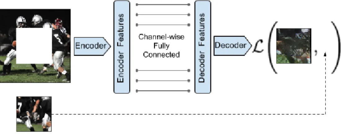
Figure 2.2: Context Encoder. The context image is passed through the encoder to obtain features which are connected to the decoder using channel-wise fully-connected layer as described in Section 2.1.1. The decoder then produces the missing regions in the image.
2.1
Context encoders for image generation
We now introduce context encoders: CNNs that predict missing parts of a scene from their surroundings. We first give an overview of the general architecture, then provide details on the learning procedure and finally present various strategies for image region removal.
2.1.1
Encoder-decoder pipeline
The overall architecture is a simple encoder-decoder pipeline. The encoder takes an input image with missing regions and produces a latent feature representation of that image. The decoder takes this feature representation and produces the missing image content. We found it important to connect the encoder and the decoder through a channel-wise fully-connected layer, which allows each unit in the decoder to reason about the entire image content. Figure 2.2 shows an overview of our architecture.
Encoder Our encoder is derived from the AlexNet architecture [128]. Given an input image of size 227×227, we use the first five convolutional layers and the following pooling layer (called pool5) to compute an abstract 6×6×256 dimensional feature representation. In contrast to AlexNet, our model is not trained for ImageNet classification; rather, the network is trained for context prediction “from scratch” with randomly initialized weights.
However, if the encoder architecture is limited only to convolutional layers, there is no way for information to directly propagate from one corner of the feature map to another. This is so because convolutional layers connect all the feature maps together, but never directly connect all locations within a specific feature map. In the present architectures, this information propagation is handled by fully-connected or inner product layers, where all the activations are directly connected to each other. In our architecture, the latent feature dimension is 6×6×256 = 9216 for both encoder and decoder. This is so because, unlike
CHAPTER 2. REPRESENTATION VIA CONTEXT PREDICTION 12
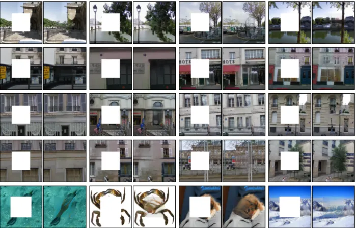
Figure 2.3: Semantic Inpainting results for context encoder trained jointly using reconstruction and adversarial loss. First four rows contain examples from Paris StreetView Dataset, and bottom row contains examples from ImageNet.
autoencoders, we do not reconstruct the original input and hence need not have a smaller
bottleneck. However, fully connecting the encoder and decoder would result in an explosion in the number of parameters (over 100M!), to the extent that efficient training on current GPUs would be difficult. To alleviate this issue, we use a channel-wise fully-connected layer to connect the encoder features to the decoder, described in detail below.
Channel-wise fully-connected layer This layer is essentially a fully-connected layer with groups, intended to propagate information within activations of each feature map. If the input layer hasm feature maps of size n×n, this layer will output m feature maps of dimension n×n. However, unlike a fully-connected layer, it has no parameters connecting different feature maps and only propagates information within feature maps. Thus, the number of parameters in this channel-wise fully-connected layer is mn4, compared tom2n4
parameters in a fully-connected layer (ignoring the bias term). This is followed by a stride 1 convolution to propagate information across channels.
Decoder We now discuss the second half of our pipeline, the decoder, which generates pixels of the image using the encoder features. The “encoder features” are connected to the “decoder features” using a channel-wise fully-connected layer.
The channel-wise fully-connected layer is followed by a series of five up-convolutional
layers [56,145,274] with learned filters, each with a rectified linear unit (ReLU) activation function. A up-convolutional is simply a convolution that results in a higher resolution image. It can be understood as upsampling followed by convolution (as described in [56]), or convolution with fractional stride (as described in [145]). The intuition behind this is straightforward – the series of up-convolutions and non-linearities comprises a non-linear weighted upsampling of the feature produced by the encoder until we roughly reach the original target size.
2.1.2
Loss function
We train our context encoders by regressing to the ground truth content of the missing (dropped out) region. However, there are often multiple equally plausible ways to fill a missing image region which are consistent with the context. We model this behavior by having a decoupled joint loss function to handle both continuity within the context and multiple modes in the output. The reconstruction (L2) loss is responsible for capturing the overall structure of the missing region and coherence with regards to its context, but tends to average together the multiple modes in predictions. The adversarial loss [81], on the other hand, tries to make prediction look real, and has the effect of picking a particular mode from the distribution. For each ground truth image x, our context encoderF produces an output
F(x). Let ˆM be a binary mask corresponding to the dropped image region with a value of 1 wherever a pixel was dropped and 0 for input pixels. During training, those masks are automatically generated for each image and training iterations, as described in Section 2.1.2. We now describe different components of our loss function.
Reconstruction Loss We use a masked L2 distance as our reconstruction loss, Lrec,
Lrec(x) = kMˆ (x−F((1−Mˆ)x))k2, (2.1)
where is the element-wise product operation. We experimented with both L1 and L2 losses and found no significant difference between them. While this simple loss encourages the decoder to produce a rough outline of the predicted object, it often fails to capture any high frequency detail (see Fig. 2.1c). This stems from the fact that the L2 (or L1) loss often prefer a blurry solution, over highly accurate textures. We believe this happens because it is much “safer” for the L2 loss to predict the mean of the distribution, because this minimizes the mean pixel-wise error, but results in a blurry averaged image. We alleviated this problem by adding an adversarial loss.
Adversarial Loss Our adversarial loss is based on Generative Adversarial Networks (GAN) [81]. To learn a generative model G of a data distribution, GAN proposes to
CHAPTER 2. REPRESENTATION VIA CONTEXT PREDICTION 14
(a)Central region (b)Random block (c) Random region
Figure 2.4: An example of image x with our different region masks ˆM applied to it.
jointly learn an adversarial discriminative model Dto provide loss gradients to the generative model. G and D are parametric functions (e.g., deep networks) where G : Z → X maps samples from noise distribution Z to data distribution X. The learning procedure is a two-player game where an adversarial discriminator D takes in both the prediction ofG and ground truth samples, and tries to distinguish them, while Gtries to confuse Dby producing samples that appear as “real” as possible. The objective for discriminator is logistic likelihood indicating whether the input is real sample or predicted one:
min
G maxD Ex∈X[log(D(x))] +Ez∈Z[log(1−D(G(z)))]
This method has shown encouraging results in generative modeling of images [200]. We thus adapt this framework for context prediction by modeling generator by context encoder; i.e., G ,F. To customize GANs for this task, one could condition on the given context information; i.e., the mask ˆM x. However, conditional GANs don’t train easily for context prediction task as the adversarial discriminator D easily exploits the perceptual discontinuity in generated regions and the original context to easily classify predicted versus real samples. We thus use an alternate formulation, by conditioning only the generator (not the discriminator) on context. We also found results improved when the generator was not conditioned on a noise vector. The GAN objective for our context encoders is as follows Hence the adversarial loss for context encoders, Ladv, is
Ladv = max
D Ex∈X[log(D(x))
+ log(1−D(F((1−Mˆ)x)))], (2.2)
where, in practice, both F and D are optimized jointly using alternating SGD. Note that this objective encourages the entire output of the context encoder to look realistic, not just the missing regions as in Equation (2.1).
Joint Loss We define the overall loss function as
L =λrecLrec+λadvLadv. (2.3)
Currently, we use adversarial loss only for inpainting experiments as AlexNet [128] architecture training diverged with joint adversarial loss. Details follow in Sections 2.3.1, 2.3.2.
Input Context Context Encoder Content-Aware Input Context Context Encoder Content-Aware Figure 2.5: Comparison with Content-Aware Fill (Photoshop feature based on [15]). Our method works better in semantic cases (top row) and works slightly worse in textured settings (bottom row).
Region masks
The input to a context encoder is an image with one or more of its regions “dropped out”; i.e., set to zero, assuming zero-centered inputs. The removed regions could be of any shape, we present three different strategies here:
Central region: The simplest such shape is the central square patch in the image, as shown in Figure 2.4a. While this works quite well for inpainting, the network learns low level image features than latch on to the boundary of the central mask. Those low level image features tend not to generalize well to images without masks, hence the features learned are not very general.
Random block: To prevent the network from latching on the the constant boundary of the masked region, we randomize the masking process. Instead of choosing a single large mask at a fixed location, we remove a number of smaller possibly overlapping masks, covering up to 14 of the image. An example of this is shown in Figure 2.4b. However, the random block masking still has sharp boundaries convolutional features could latch onto.
Random region: To completely remove those boundaries, we experimented with removing arbitrary shapes from images, obtained from random masks in the PASCAL VOC 2012 dataset [62]. We deform those shapes and paste in arbitrary places in the other images (not from PASCAL), again covering up to 14 of the image. Note that we completely randomize the region masking process, and do not expect or want any correlation between the source segmentation mask and the image. We merely use those regions to prevent the network from learning low-level features corresponding to the removed mask. See example in Figure 2.4c. In practice, we found region and random block masks produce a similarly general feature, while significantly outperforming the central region features. We use the random region dropout for all our feature based experiments.
2.2
Implementation details
The pipeline was implemented inCaffe[112] and Torch. We used ADAM [119] for optimization. The missing region in the masked input image is filled with constant mean value. Hyper-parameter details are discussed in Sections 2.3.1, 2.3.2. We experimented with replacing all pooling layers with convolutions of the same kernel size and stride. The overall stride of the
CHAPTER 2. REPRESENTATION VIA CONTEXT PREDICTION 16
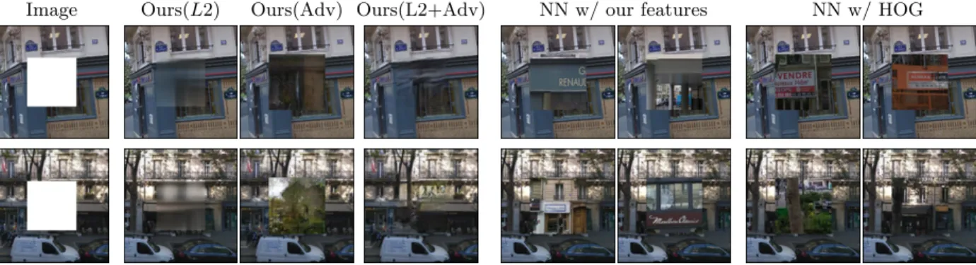
Image Ours(L2) Ours(Adv) Ours(L2+Adv) NN w/ our features NN w/ HOG
Figure 2.6: Semantic Inpainting using different methods. Context Encoder with just L2 are well aligned, but not sharp. Using adversarial loss, results are sharp but not coherent. Joint loss alleviate the weaknesses of each of them. The last two columns are the results if we plug-in the best nearest neighbor (NN) patch in the masked region.
Method Mean L1 Loss Mean L2 Loss PSNR (higher better)
NN-inpainting (HOG features) 19.92% 6.92% 12.79 dB
NN-inpainting (our features) 15.10% 4.30% 14.70 dB
Our Reconstruction (joint) 10.33% 2.35% 17.59 dB
Table 2.1: Semantic Inpainting accuracy for Paris StreetView dataset on held-out images. NN inpainting is basis for [93].
network remains the same, but it results in finer inpainting. Intuitively, there is no reason to use pooling for reconstruction based networks. In classification, pooling provides spatial invariance, which may be detrimental for reconstruction-based training. To be consistent with prior work, we still use the original AlexNet architecture (with pooling) for all feature learning results.
2.3
Evaluation
We now evaluate the encoder features for their semantic quality and transferability to other image understanding tasks. We experiment with images from two datasets: Paris StreetView [52] and ImageNet [205] without using any of the accompanying labels. In Section 2.3.1, we present visualizations demonstrating the ability of the context encoder to fill in semantic details of images with missing regions. In Section 2.3.2, we demonstrate the transferability of our learned features to other tasks, using context encoders as a pre-training step for image classification, object detection, and semantic segmentation. We compare our results on these tasks with those of other unsupervised or self-supervised methods, demonstrating that our approach outperforms previous methods.
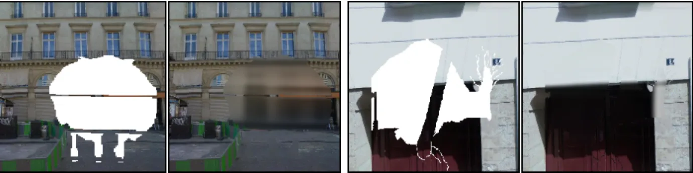
Figure 2.7: Arbitrary region inpainting for context encoder trained with reconstruction loss.
2.3.1
Semantic Inpainting
We train context encoders with the joint loss function defined in Equation (2.3) for the task of inpainting the missing region. The encoder and discriminator architecture is similar to that of discriminator in [200], and decoder is similar to generator in [200]. However, the bottleneck is of 4000 units (in contrast to 100 in [200]); see supplementary material. We used the default solver hyper-parameters suggested in [200]. We use λrec = 0.999 and λadv = 0.001. However,
a few things were crucial for training the model. We did not condition the adversarial loss (see Section 2.1.2) nor did we add noise to the encoder. We use a higher learning rate for context encoder (10 times) to that of adversarial discriminator. To further emphasize the consistency of prediction with the context, we predict a slightly larger patch that overlaps with the context (by 7px). During training, we use higher weight (10×) for the reconstruction loss in this overlapping region.
The qualitative results are shown in Figure 2.3. Our model performs generally well in inpainting semantic regions of an image. However, if a region can be filled with low-level textures, texture synthesis methods, such as [15,61], can often perform better (e.g. Figure 2.5). For semantic inpainting, we compare against nearest neighbor inpainting (which forms the basis of Hays et al. [93]) and show that our reconstructions are well-aligned semantically, as seen on Figure 2.6. It also shows that joint loss significantly improves the inpainting over both reconstruction and adversarial loss alone. Moreover, using our learned features in a nearest-neighbor style inpainting can sometimes improve results over a hand-designed distance metrics. Table 2.1 reports quantitative results on StreetView Dataset.
2.3.2
Feature Learning
For consistency with prior work, we use the AlexNet [128] architecture for our encoder. Unfortunately, we did not manage to make the adversarial loss converge with AlexNet, so we used just the reconstruction loss. The networks were trained with a constant learning rate of 10−3 for the center-region masks. However, for random region corruption, we found
a learning rate of 10−4 to perform better. We apply dropout with a rate of 0.5 just for the
CHAPTER 2. REPRESENTATION VIA CONTEXT PREDICTION 18
Ours Ours
HOG HOG
AlexNet AlexNet
Figure 2.8: Context Nearest Neighbors. Center patches whose context (not shown here) are close in the embedding space of different methods (namely our context encoder, HOG and AlexNet). Note that the appearance of these center patches themselves was never seen by these methods. But our method brings them close just from their context.
be prone to overfitting. The training process is fast and converges in about 100K iterations: 14 hours on a Titan X GPU. Figure 2.7 shows inpainting results for context encoder trained with random region corruption using reconstruction loss. To evaluate the quality of features, we find nearest neighbors to the masked part of image just by using the features from the context, see Figure 2.8. Note that none of the methods ever see the center part of any image, whether a query or dataset image. Our features retrieve decent nearest neighbors just from context, even though actual prediction is blurry with L2 loss. AlexNet features also perform decently as they were trained with 1M labels for semantic tasks, HOG on the other hand fail to get the semantics.
Classification pre-training
For this experiment, we fine-tune a standard AlexNet classifier on the PASCAL VOC 2007 [62] from a number of supervised, self-supervised and unsupervised initializations. We train the classifier using random cropping, and then evaluate it using 10 random crops per test image. We average the classifier output over those random crops. Table 2.2 shows the standard mean average precision (mAP) score for all compared methods. A random initialization performs roughly 25% below an ImageNen-trained model; however, it does not use any labels. Context encoders are competitive with concurrent self-supervised feature learning methods [51,254] and significantly outperform autoencoders and Agrawal et al. [4].
Detection pre-training
Our second set of quantitative results involves using our features for object detection. We use
Fast R-CNN [80] framework (FRCN). We replace the ImageNet pre-trained network with our context encoders (or any other baseline model). In particular, we take the pre-trained encoder weights up to the pool5 layer and re-initialize the fully-connected layers. We then
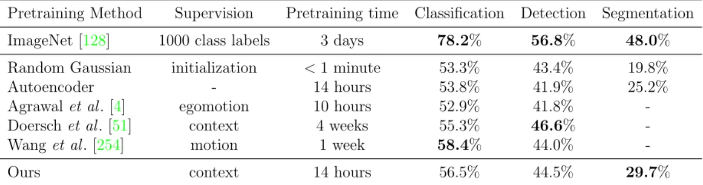
Pretraining Method Supervision Pretraining time Classification Detection Segmentation ImageNet [128] 1000 class labels 3 days 78.2% 56.8% 48.0% Random Gaussian initialization <1 minute 53.3% 43.4% 19.8%
Autoencoder - 14 hours 53.8% 41.9% 25.2%
Agrawalet al. [4] egomotion 10 hours 52.9% 41.8% -Doerschet al. [51] context 4 weeks 55.3% 46.6%
-Wanget al. [254] motion 1 week 58.4% 44.0%
-Ours context 14 hours 56.5% 44.5% 29.7%
Table 2.2: Quantitative comparison for classification, detection and semantic segmentation. Clas-sification and Fast-RCNN Detection results are on the PASCAL VOC 2007 test set. Semantic segmentation results are on the PASCAL VOC 2012 validation set from the FCN evaluation de-scribed in Section 2.3.2, using the additional training data from [90], and removing overlapping images from the validation set [145].
follow the training and evaluation procedures from FRCN and report the accuracy (in mAP) of the resulting detector.
Our results on the test set of the PASCAL VOC 2007 [62] detection challenge are reported in Table 2.2. Context encoder pre-training is competitive with the existing methods achieving significant boost over the baseline. Kr¨ahenb¨uhlet al. [126] proposed a data-dependent method for rescaling pre-trained model weights. This significantly improves the features in Doerschet al. [51] up to 65.3% for classification and 51.1% for detection. However, this rescaling doesn’t improve results for other methods, including ours.
Semantic Segmentation pre-training
Our last quantitative evaluation explores the utility of context encoder training for pixel-wise semantic segmentation. Fully convolutional networks [145] (FCNs) were proposed as an end-to-end learnable method of predicting a semantic label at each pixel of an image, using a convolutional network pre-trained for ImageNet classification. We replace the classification pre-trained network used in the FCN method with our context encoders, afterwards following the FCN training and evaluation procedure for direct comparison with their originalCaffeNet -based result.
Our results on the PASCAL VOC 2012 [62] validation set are reported in Table 2.2. In this setting, we outperform a randomly initialized network as well as a plain autoencoder which is trained simply to reconstruct its full input.
2.4
Related work
CNNs trained for ImageNet [205] classification with over a million labeled examples learn features which generalize very well across tasks [53]. However, whether such semantically
CHAPTER 2. REPRESENTATION VIA CONTEXT PREDICTION 20
informative and generalizable features can be learned from raw images alone, without any labels, remains an open question. Unsupervised learning is a broad area with a large volume of work; Bengio et al. [20] provide an excellent survey. Here, we briefly revisit some of the recent work in this area.
Self-supervision via pretext tasks Instead of producing images, several recent studies have focused on providing alternate forms of supervision (often called ‘pretext tasks’) that do not require manual labeling and can be algorithmically produced. For instance, Doersch
et al. [51] task a ConvNet with predicting the relative location of two cropped image patches. Noroozi and Favaro [164] extend this by asking a network to arrange shuffled patches cropped from a 3×3 grid. Other pretext tasks include predicting color channels from luminance [132,276] or vice versa [277], and predicting sounds from video frames [46,175]. The assumption in these works is that to perform these tasks, the network will need to recognize high-level concepts, such as objects, in order to succeed.
Most closely related to our idea are efforts at exploiting spatial context as a source of free and plentiful supervisory signal. Visual Memex [149] used context to non-parametrically model object relations and to predict masked objects in scenes, while [50] used context to establish correspondences for unsupervised object discovery. However, both approaches relied on hand-designed features and did not perform any representation learning. Doersch et al. [51] used the task of predicting the relative positions of neighboring patches within an image as a way to train an unsupervised deep feature representations. We share the same high-level goals with Doersch et al. but fundamentally differ in the approach: whereas [51] are solving a discriminative task (is patch A above patch B or below?), our context encoder solves a pureprediction problem (what pixel intensities should go in the hole?). Interestingly, similar distinction exist in using language context to learn word embeddings: Collobert and Weston [38] advocate a discriminative approach, whereas word2vec [151] formulate it as word prediction. One important benefit of our approach is that our supervisory signal is much richer: a context encoder needs to predict roughly 15,000 real values per training example, compared to just 1 option among 8 choices in [51]. Likely due in part to this difference, our context encoders take far less time to train than [51]. Moreover, context based prediction is also harder to “cheat” since low-level image features, such as chromatic aberration, do not provide any meaningful information, in contrast to [51] where chromatic aberration partially solves the task. On the other hand, it is not yet clear if requiring faithful pixel generation is necessary for learning good visual features.
Unsupervised learning by generating images Classical unsupervised representation learning approaches, such as autoencoders [19,99] and denoising autoencoders [248], attempt to learn feature representations from which the original image can be decoded with a low error. An alternative to reconstruction-based objectives is to train generative models of images using generative adversarial networks [81]. These models can be extended to produce good feature representations by training jointly with image encoders [54,59]. However, to
generate realistic images, these models must pay significant attention to low-level details while potentially ignoring higher-level semantics. We train our context encoders using an adversary jointly with reconstruction loss for generating inpainting results. We discuss this in detail in Section 2.1.2.
Dosovitskiy et al. [56] and Rifaiet al. [202] demonstrate that CNNs can learn to generate novel images of particular object categories (chairs and faces, respectively), but rely on large labeled datasets with examples of these categories. In contrast, context encoders can be applied to any unlabeled image database and learn to generate images based on the surrounding context.
Inpainting and hole-filling It is important to point out that our hole-filling task cannot be handled by classical inpainting [22,170] or texture synthesis [15,61] approaches, since the missing region is too large for local non-semantic methods to work well. In computer graphics, filling in large holes is typically done via scene completion [93], involving a cut-paste formulation using nearest neighbors from a dataset of millions of images. However, scene completion is meant for filling in holes left by removing whole objects, and it struggles to fill arbitrary holes, e.g. amodal completion of partially occluded objects. Furthermore, previous completion relies on a hand-crafted distance metric, such as Gist [167] for nearest-neighbor computation which is inferior to a learned distance metric. We show that our method is often able to inpaint semantically meaningful content in a parametric fashion, as well as provide a better feature for nearest neighbor-based inpainting methods.