Network effects, nonlinear pricing and entry deterrence
Arun Sundararajan
1Leonard N. Stern School of Business, New York University 44 West 4th Street, KMC 8-93 New York, NY 10012
First Draft: January 2003
This Draft: July 2003
Abstract: A number of products that display positive network effects are used in variable quantities by heterogeneous customers. Examples include corporate operating systems, infrastructure software, web services and networking equipment. In many of these contexts, the magnitude of network effects are infl u-enced by gross consumption, rather than simply by user base. Moreover, the value an individual customer derives on account of these network effects may be related to the extent of their individual consumption, and therefore, the network effects may be heterogeneous across customers.
This paper presents a model of nonlinear pricing in the presence of such network effects, under incomplete information, and with the threat of competitive entry. Both homogeneous and heterogeneous network effects are modeled. Conditions under which a fulfilled-expectations contract exists and is unique are established. While network effects generally raise prices, it is shown that accompanying changes in consumption depend on the nature of the network effects — in some cases, it is optimal for the monopolist to induce no changes in usage across customers, while in others cases, network effects raise the usage of all market participants. Optimal pricing is shown to include quantity discounts that increase with usage, and may also involve a nonlinear two-part tariff. These results highlight the impact of network effects on the standard trade-off between price discrimination and value creation, and have important implications for pricing policy.
The threat of entry generally lowers profits for the monopolist, and increases customer surplus. When network effects are homogeneous across customers, the resulting entry-deterring monopoly contract is afixed fee and results in the socially optimal outcome. However, when the magnitude of heterogeneous network effects is relatively high, there are no changes in total surplus induced by the entry threat, and the price changes merely cause a transfer of value from the seller to its customers. The presence of network effects, and of a credible entry threat, are also shown to increase distributional efficiency by reducing the disparity in relative value captured by different customer types. Regulatory and policy implications of these results are discussed.
JEL Classification: D42, L11, L12 1
I thank Luis Cabral, Nicholas Economides, Ravi Mantena and Roy Radner for helpful discussions, seminar par-ticipants at New York University, and conference parpar-ticipants at the 2003 meeting of the Society for the Advancement of Economic Theory for their feedback. All responsibility for errors and omissions remain mine.
1. Introduction
This paper presents a model in which products displays positive network effects, individual con-sumption varies across heterogeneous customers, and the magnitude of network effects depend on gross consumption. The principal goals of the paper are to characterize the optimal nonlinear pric-ing schedules for different kinds of network effects, and under the potential threat of competitive entry, and to study their consumption and welfare properties.
Standard theories of network effects typically assume that each customer purchases a maximum of one unit of the product, that the value of the network effect is proportionate to the total size of the product’s eventual user base, and that all customer benefit equally from the network effects (Katz and Shapiro, 1985, Farrell and Saloner, 1985). However, there are a number of products that display network effects (henceforth termed network goods) which are consumed in variable quantities by different customers, and for which the magnitude of the network effects may depend on the total quantity consumed across customers, rather than simply the total number of adopters. In addition, the value each customer derives from the network good may depend on their individual consumption, which in turn depends on the intrinsic value they place on the product. Extending the standard theory to incorporate these observations may have important implications for companies seeking to design optimal pricing policy for their network goods, as well as for the regulatory analysis of industries with network effects.
The relevance of these observations can be illustrated through a few common examples of products that display network effects. Consider, for instance, the purchase of PC operating systems software by corporate customers. The (simplest) pricing problem faced by a seller in this market is one of choosing a pricing schedule, where quantity is measured by number of user licenses, and each corporate customer purchases a variable quantity of licenses. The network effects are caused largely by the higher availability and quality of complementary goods (applications software, compatible accessories) as the total number of OS installations increases. Consequently, the magnitude of the network effects are proportionate to the total number of licenses sold (the gross consumption), rather than simply the number of corporations who adopt the OS. Moreover, a corporation which has a higher number of licenses benefits more from the increased quality and availability of the complementary goods — in other words, the value realized from the network effects also depends on individual consumption, and may therefore be heterogeneous across corporations2.
A similar argument can be made for back-end or enterprise software used in variable quantities by different companies (Oracle’s database software and Siebel’s CRM software being two examples),
2
In addition, there is a positive externality driven by value from interoperability, which is far more important within an organization than across companies, and is therefore influenced more by individual consumption.
or for networking equipment like routers and switches. In these cases, network effects are driven by the ease with which one canfind qualified support or administration engineers, trained employ-ees, compatible software, or compatible equipment3. Network goods sold directly to individuals consumers may also display the same properties. For example, electronic marketplaces like eBay are widely recognized as displaying positive network effects, which stem from increased liquidity, as well as a wider availability of robust systems supporting marketplace services (reputation, escrow, payment, settlement, dispute resolution). The magnitude of the network effects increases not just with the number of participants in the market, but with the extent to which each participant ac-tually buys and sells; moreover, an individual who participates more realizes higher benefits from them. Even for products used as canonical examples of network goods, such as telephone service, usage varies across consumers, network effects dependent on total consumption as well as installed base, users with higher consumption levels benefit more from the network effects, and pricing is often nonlinear.
The ubiquity of variable consumption and heterogenous value from network goods underlines the importance of developing a model that incorporates these properties. This paper provides such an model, characterizing the optimal nonlinear pricing schedule for a monopolist selling a network good which explicitly displays the properties highlighted in the examples above. Two cases are analyzed successively. First, network effects whose magnitude depends on gross realized consumption (and are homogeneous across customers) are studied. Subsequently, network effects whose magnitude is heterogeneous across customers (by virtue of depending on both gross consumption and individual consumption) are modeled. The changes in consumption induced by the network effects are shown to vary significantly across the cases. There are also interesting variations in the manner in which the value generated by the network effects is distributed across the different customers. Moreover, while there are progressively steeper quantity discounts as individual consumption increases in both cases, optimal pricing in the latter case may involve a two-part tariff.
In addition to pure monopoly pricing, this paper also analyzes pricing by an entry-deterring monopolist. Many markets for technology goods feature dominant sellers with market power, and there has been substantial recent interest in whether (and how) the potential threat of entry affects their pricing choices. For instance, in the recent U.S. versus Microsoft case, both parties agreed that Microsoft’s pricing was not consistent with monopoly profit maximization, and Schmalensee (1999) argued that Microsoft underprices in order to reduce the desirability of entry by competing firms into the market for operating systems. Fudenberg and Tirole (2000) develop a formal model 3While open networking standards do form the basis for most networking equipment, many vendors like Cisco Systems use proprietary operating systems. Moreover, the ease of interoperability between equipment from competing vendors varies widely.
of limit pricing that supports this argument, in which installed base plays an entry-deterring role analogous to that of excess capacity (Spence, 1977, Dixit, 1980).
This paper proposes and analyzes an alternate representation, in which to successfully deter a threat of entry, the monopolist must provide each customer with surplus equal to at least the maximum intrinsic value they could get from a competing product. This limits the price each customer pays under the monopolist’s nonlinear pricing schedule to being no more than the network value they get from the monopolist’s product. As a consequence, network value may play the role of being the primary source of profits for a monopolist who prices to successfully deter entry. On the face of it, this has promising welfare implications, since one would expect a threat of entry to induce a substantial increase in consumption. Surprisingly, it is shown that there are sometimes no consumption changes (despite price reductions), and that when there are, the consumption increases are confined largely to a lower subset of types. However, entry deterrence is shown to even out the relative distribution of surplus across different customer types.
This paper draws from and adds to two lines of research. Thefirst is the literature on monopoly pricing of technology products with positive network externalities. Related papers with monopoly models include Rohlfs (1974), Oren, Smith and Wilson (1982), Economides (1996a), and Cabral, Salant and Woroch (1999). Modeling network goods for which the network effects depend on gross consumption (rather than the number of adopters) is new, as is the analysis of heterogeneity in the value of the network effects across customers. The concept of fulfilled-expectations equilibrium is extended to the case of customers purchasing variable quantities in a monopoly market. A related area of research is the literature on monopoly withnegative consumption externalities, specifically in the context of congestion in queuing and service systems (Mendelson, 1985, Dewan and Mendelson, 1990, Mendelson and Whang, 1990, Westland, 1992).
The second line of research this paper adds to is the literature on single-dimensional price screening. It contributes new results to the theory by characterizing how positive network effects of different kinds affect optimal nonlinear pricing, and by establishing conditions under which optimal nonlinear pricing schedules that satisfy fulfilled-expectations exist and are unique. It complements recent work by Segal and Whinston (2001), and by Jullien (2001), that examine different problems of optimal contracting in the presence of network externalities.
The rest of this paper is organized as follows. Section 2 specifies the basic model, defines the solution concept, and characterizes the model’s description of entry deterrence. Section 3 presents the analysis of the monopoly with homogeneous network effects, and Section 4 analyzes the case of heterogeneous network effects. Both sections 3 and 4 examine pricing and consumption changes induced by network effects, examine some welfare properties, establish how nonlinear pricing is
affected by the threat of entry, and conclude with a simple example that illustrates the nature of the optimal pricing schedule and surplus distribution. Section 5 discusses the results further, discusses the model’s assumptions, and concludes with an outline of open research questions raised.
2. Model
2.1. Firm and customers
A monopolist sells a homogeneous product which may be used by consumers in varying quantities. The variable costs of production are assumed to be zero (though Section 5.2 describes how the model’s results are robust to relaxing this assumption). Customers are heterogeneous, indexed by their typeθ ∈[θ,θ]. The monopolist does not observe the type of any customer, but knows F(θ), the probability distribution of types in the customer population. F(θ) is assumed to be strictly increasing and absolutely continuous, and therefore the corresponding density functionf(θ) exists and is strictly positive for all θ ∈ [θ,θ]. In addition, 1−f(Fθ()θ), the reciprocal of the hazard rate, is assumed to be non-increasing for allθ. Each customer knows their own typeθ. The total number of customers in the market is normalized to1.
The preferences of a customer of typeθare represented by the linearly separable utility function
V(q,θ, Q, p) =W(q,θ, Q)−p, (2.1)
where q is the quantity of the product used by the customer (often referred to as individual con-sumption),Qis the total quantity of the product used by all customers in the market (often referred to as the gross consumption) and p is the total price paid by the customer. W(q,θ, Q) is often referred to as the value function.
The value function whenQ= 0 is denotedU(q,θ), and is referred to as theintrinsic value from the network good for customer typeθ. That is:
U(q,θ) =W(q,θ,0) (2.2)
for all q,θ. At any positive Q, the expression [W(q,θ, Q)−U(q,θ)] is referred to as thenetwork value from the network good for customer typeθ.
The value functionW(q,θ, Q) is assumed to have the following properties:
1. W11(q,θ, Q)<0,W2(q,θ, Q)>0,W12(q,θ, Q)>0. 2. W3(q,θ, Q)≥0, W13(q,θ, Q)≥0,W23(q,θ, Q)≥0
3. d dθ( −W11(q,θ, Q) W1(q,θ, Q) )<0,W122(q,θ, Q)≤0. 4. β(θ, Q) = arg max
q W(q,θ, Q) is finite and unique for all θ. W1(q,θ, Q) > 0 forq < β(θ, Q), and W1(q,θ, Q)<0 for q >β(θ, Q).
Numbered subscripts to functions denote partial derivatives with respect to the corresponding variable. Thefirst set of properties — strict concavity inq, increasing value with type, and increasing marginal value with type (the Spence-Mirrlees single-crossing condition) — are common assumptions in models of nonlinear pricing. The second set of properties characterizes the nature of the network effects — the gross value from the network effects is non-decreasing in gross consumption, and the marginal value from an increase in gross consumption is (weakly) higher at a higher level of individual consumption, and is (weakly) higher for higher types. The source of these network effects are not modeled explicitly. The model therefore adopts what Economides (1996b) calls the ‘macro’ approach.
The third set of properties assume decreasing absolute risk aversion (which is frequently used to characterize the relative curvature of the value functions of different customer types), and marginal utility that is concave in type θ (which is a standard assumption to ensures that the optimal contract separates customer types). In one case, a slightly stronger assumption than decreasing absolute risk aversion — that the concavity ofW with respect toq does not increase with type — is necessary4.
The final set of properties simply state that there is a consumption level beyond which the value from additional consumption decreases. It reflects the reality that customers consume a finite quantity of any network good, even if the marginal price of additional consumption is zero (under a site license, for instance). This is because value from usage is typically bounded by a constraint on some related resource — attention or computing power being two common examples — and the implicit presence of a substitute use for this resource. Analogously, sometimes the increased consumption of the product may necessitate the purchase of additional necessary complementary assets (more powerful computer hardware for increased software usage, for instance)5. The quantity that maximizesintrinsic value is denotedα(θ) — that is,α(θ) =β(θ,0).
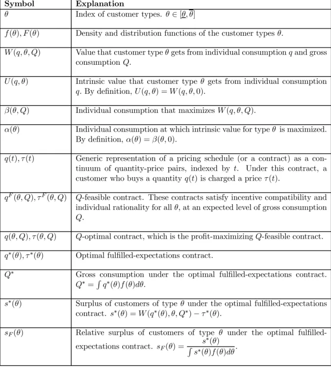
Each customer of type θ is assumed to have reservation utility ˆU(θ)≥0. The functions F(θ), W(q,θ, Q), U(q,θ), and ˆU(θ) are common knowledge. Notation used most frequently (some of which is defined formally later in the paper) is summarized in Table 2.1.
4
IfW1(q,θ, Q)>0, thenW112(q,θ, Q)≥0 implies that ddθ(−W11(q,θ,Q)
W1(q,θ,Q) )<0. 5
See Sundararajan (2002), Section 4, for more discussion and examples. Also Section 5.2 of the current paper discusses relaxing this assumption in the presence of convex costs.
Symbol Explanation
θ Index of customer types. θ∈[θ,θ]
f(θ), F(θ) Density and distribution functions of the customer types θ.
W(q,θ, Q) Value that customer typeθgets from individual consumptionqand gross consumption Q.
U(q,θ) Intrinsic value that customer type θ gets from individual consumption q. By definition,U(q,θ) =W(q,θ,0).
β(θ, Q) Individual consumption that maximizes W(q,θ, Q).
α(θ) Individual consumption at which intrinsic value for typeθ is maximized. By definition, α(θ) =β(θ,0).
q(t),τ(t) Generic representation of a pricing schedule (or a contract) as a con-tinuum of quantity-price pairs, indexed by t. Under this contract, a customer who buys a quantity q(t) is charged a priceτ(t).
qF(θ, Q),τF(θ, Q) Q-feasible contract. These contracts satisfy incentive compatibility and individual rationality for allθ,at an expected level of gross consumption Q.
q(θ, Q),τ(θ, Q) Q-optimal contract, which is the profit-maximizingQ-feasible contract. q∗(θ),τ∗(θ) Optimal fulfilled-expectations contract.
Q∗ Gross consumption under the optimal fulfilled-expectations contract. Q∗ =R q∗(θ)f(θ)dθ.
s∗(θ) Surplus of customers of type θ under the optimal fulfilled-expectations
contract. s∗(θ) =W(q∗(θ),θ, Q∗)−τ∗(θ).
sF(θ) Relative surplus of customers of type θ under the optimal fulfi lled-expectations contract. sF(θ) = s
∗(θ)
R
s∗(θ)f(θ)dθ.
The monopolist chooses a pricing schedule (also called a contract) which specifies a price for each level of individual consumptionq. Since the monopolist cannot explicitly distinguish between customer types prior to contracting, the entire menu of quantity-price pairs must be available to all customers. Rather than explicitly considering all possible pricing functions, the revelation principle ensures that we can restrict our analysis todirect mechanisms which specify the pricing schedule as a menu of quantity-price pairs (q(t),τ(t)), where where t∈[θ,θ], which are incentive-compatible.
2.2. Sequence of events
The interaction between the monopolist and their customers is according to the following sequence:
1. The monopolist announces their pricing schedule as a menu of quantity-price pairsq(t),τ(t). 2. Customers observeq(t),τ(t), and form an expectation about what the gross consumption un-der this pricing schedule will be. All customers have access to the same relevant information6, and are assumed to form the same expectationQE, which is also known to the monopolist. 3. Based on their typeθand the expectation of gross consumptionQE, each customer determines
their optimal individual consumptionq(t(θ)), wheret(θ) = arg max
t [W(q(t),θ, Q E)
−τ(t)]. If the customer gets at least their reservation utility, that is, if:
W(q(t(θ)),θ, QE)−τ(t(θ))≥U(θ),ˆ (2.3)
then the customer chooses to consumeq(t(θ)) and payτ(t(θ)). If not, the customer does not participate, and purchases zero quantity.
4. The monopolist gets a payoffof Z
θ∈Θ
τ(t(θ))f(θ)dθ, (2.4)
whereΘis the set of participating types. Each participating customer gets a payoffof
W(q(t(θ)),θ, QA)−τ(t(θ)), (2.5)
whereQAis the actual realized gross consumption. Each customer that does not participate gets a payoffof ˆU(θ).
6The customer’s unique knowledge of their own type does not affect their expectation of gross consumption, which is completely determined byf(θ), the pricing schedule, and the functionsU(q,θ),W(q,θ, Q), and ˆU(θ) (all of which are common knowledge at this stage).
2.3. Contracts
This subsection defines the different contracts that are used in subsequent analysis. To simplify notation, the definition of the following contracts is based on the assumption of full participation — that is, that all customers find it optimal to purchase under the contract, if it specifies a non-negative allocation for their type. In sections 3 and 4, inducing full participation is always optimal for the monopolist.
Q-feasible contracts: Given any expectation of gross consumption Q, a Q-feasible contract is a menu of of quantity-price pairs (qF(t, Q),τF(t, Q)) which satisfies incentive-compatibility [IC] and individual rationality [IR]:
[IC] : θ= arg max
t W(q
F(t, Q),θ, Q)
−τF(t, Q) ∀θ (2.6)
[IR] : W(qF(θ, Q),θ, Q)−τF(θ, Q)≥Uˆ(θ) ∀θ (2.7)
Q-optimal contracts: Given any expectation of gross consumptionQ, anQ-optimal contract (q(θ, Q),τ(θ, Q)) is aQ-feasible contract that solves the monopolist’s profit maximization problem:
max qF(t,Q),τF(t,Q) θ Z θ τF(t, Q)f(t)dt, (2.8)
over all (qF(t, Q),τF(t, Q)) that satisfy [IC] and [IR].
Optimal fulfilled-expectations contracts: A optimal fulfilled-expectations contract is a menu of price-quantity pairsq∗(θ),τ∗(θ) such that the contract q(θ, Q),τ(θ, Q) defined by
Q = θ Z θ q∗(θ)f(θ)dθ q(θ, Q) = q∗(θ) (2.9) τ(θ, Q) = τ∗(θ) is aQ-optimal contract.
Based on the definitions above, note that if any Q-optimal contract q(θ, Q),τ(θ, Q) satisfies fulfilled-expectations [FE] for someQ:
[F E] :Q= θ
Z
θ
then the contract q∗(θ) =q(θ, Q),τ∗(θ) =τ(θ, Q) is an optimal fulfilled-expectations contract. The solution that the monopolist seeks is a optimal fulfilled-expectations contract. The con-ditions for the existence and possible uniqueness of these contracts are described independently in each subsection.
2.4. Entry deterrence and participation constraints
The monopolist in the model may face a threat of entry from an entrant7, whose product is intrinsically a perfect substitute for the monopolist’s product. By virtue of being the incumbent, the monopolist’s product generatespositive network value for all customers. The entrant’s product, on the other hand, is assumed to provide only its intrinsic value to the customers. Thefixed cost of entry is assumed to be zero.
The purpose of this subsection is to establish that the problem of pricing to deter entry under the threat of costless entry is equivalent to a problem of pricing in the absence of the entry threat, but instead with specific type-dependent individual rationality constraints.
At a gross consumption level Q, the utility of a customer of type θ who purchases a quantity q of the monopolist’s product for a paymentp is (W(q,θ, Q)−p), and the utility of a customer of type θwho purchases a quantityq of the entrant’s product for a paymentpis (U(q,θ)−p). Given a set of prices, and an expectationQof gross consumption of the monopolist’s product, customers choose the product and quantity that maximizes their utility. Customers indifferent between the monopolist’s and the entrant’s products are assumed to choose the monopolist’s product.
A complete characterization of the entry game is not provided. Rather, the analysis focuses on the characteristics of pricing schedules for the monopolist that successfully deter entry. Since thefixed cost of entry is assumed to be zero, these are pricing schedules for the monopolist under which any pricing schedule offered by the entrant results in zero profits for the entrant.
Recall that α(θ) = arg max q U(q,θ), (2.11) and that β(θ, Q) = arg max q W(q,θ, Q). (2.12)
Suppose the entrant offered the constant pricing scheme p(q) = ε, where ε is small. Under this pricing scheme, each customer would choose their intrinsic-value maximizing level of consumption α(θ), and would realize surplus of (U(α(θ),θ)−ε). If customers of typeθ expected surplus of less
than (U(α(θ),θ)−ε) from the monopolist’s product, they would buy the entrant’s product, and the entrant would receive non-zero profits. Therefore, in order to deter entry, the monopolist’s pricing scheme must provide customers of typeθ with a surplus of at least (U(α(θ),θ)−ε), for all ε>0. Clearly, this cannot be achieved unless the monopolist’s pricing scheme provides customers of type θ with surplus of at leastU(α(θ),θ). Since U(α(θ),θ) is the maximum surplus that a customer of type θ can get from the entrant’s product underany pricing scheme, ensuring that customers get this level of surplus is both necessary and sufficient for the monopolist to deter entry.
As a consequence, when the fixed cost of entry is zero, deterring entry simply imposes a lower bound on the surplus each customer type must receive. Analytically, this is identical to the problem of choosing a pricing scheme withtype-dependent individual rationality constraints (Jullien, 2000). In other words, setting ˆU(θ) = U(α(θ),θ) in equation (2.7) ensures that any Q-feasible contract deters entry, and the definitions of all the other contracts in section 2.3 remain the same.
When faced with a threat of entry, the monopolist’s problem is therefore to choose the optimal fulfilled-expectations contract, with ˆU(θ) =U(α(θ),θ). In the following sections, the monopolist’s problem is solved both in the absence of an entry threat, as well as in its presence, for both homogeneous and heterogeneous network effects.
2.5. Preliminary results
The purpose of this subsection is to present two preliminary results used in the subsequent analysis. The first result characterizes the optimal contract offered by the monopolist in the absence of network effects — that is, when W(q,θ, Q) =U(q,θ) for all Q. This is termed thebase case, and is used as a benchmark in sections 3 and 4. The second result describes the structure of Q-optimal contracts, and demonstrates their uniqueness.
In the base case, since there are no network effects, fulfilled-expectations do not play a role.
Lemma 1. When W(q,θ, Q) =U(q,θ), the monopolist offers the contract q0(θ),τ0(θ) which
sat-isfies the following conditions for all θ:
U1(q0(θ),θ) U12(q0(θ),θ) = 1−F(θ) f(θ) ; (2.13) τ0(θ) = U(q0(θ),θ)− θ Z θ U2(q0(x), x)dx (2.14)
This contract defined by (2.13) and (2.14) is unique. Moreover, for all θ such that q0(θ) >0, it satisfiesq01(θ)>0,τ01(θ)>0.
The proof of this result is omitted. The reader is referred to chapter 2 of Salani´e (1997) for a simple exposition, or to Maskin and Riley (1984) for more details. A complete proof based on a model formulation similar to that of this paper is also available in Sundararajan (2002).
Lemma 2. IfUˆ(θ) = 0, for every expectation of consumptionQ, theQ-optimal contractq(θ, Q),τ(θ, Q)
is unique, and is defined by the following conditions:
W1(q(θ, Q),θ, Q) W12(q(θ, Q),θ, Q) = 1−F(θ) f(θ) , (2.15) and τ(θ, Q) =W(q(θ, Q),θ, Q)− θ Z θ W2(q(θ, Q), x, Q)dx. (2.16)
Unless otherwise specified, proofs of all results are available in Appendix A.
3. Homogeneous network e
ff
ects
This section analyzes network effects that depend on just gross consumption, and discusses some properties of consumption, pricing and welfare under the optimal fulfilled-expectations contract. The value function W(q,θ, Q) is assumed to be linearly separable in intrinsic value and network value, and to take the following form
W(q,θ, Q) =U(q,θ) +w(Q). (3.1)
From the definition of intrinsic valueU(q,θ), (3.1) implies thatw(0) = 0.
3.1. Pure monopoly pricing
In the absence of an entry threat (which is referred to as pure monopoly, to distinguish it from the subsequent entry-deterring monopoly), the following proposition establishes that the unique solution to the monopolist’s problem is very similar to that of the base case:
Proposition 1. If W(q,θ, Q) = U(q,θ) +w(Q), then the optimal fulfilled-expectations contract takes the form:
q∗(θ) = q0(θ); (3.2)
1 * q (q ) 1( , 2) U qq 2 12 2 2 1 ( ) ( , ) ( ) F U q f - q q q 1 12 1 1 1 ( ) ( , ) ( ) F U q f - q q q 1( , )1 U qq 2 * q (q ) 1 1 12 12 W ( q, ,Q ) U ( q, ) W ( q, ,Q ) U ( q, ) q = q q = q
Figure 3.1: Illustrates the optimal consumption of two typesθ1andθ2(θ1 <θ2) withhomogeneous network effects under pure monopoly. First-order necessary conditions are met for each type at the intersection of the U1(q,θ) and the U12(q,θ)1−fF(θ()θ) curves. As a consequence,q∗(θ) =q0(θ).
where q0(θ) and τ0(θ) are specified in (2.13) and (2.14), and Q0 = Rθ θ
q0(θ)f(θ)dθ. A contract of
this form exists and is unique for any functionw(Q).
Proposition 1 shows that when the network value function depends on just gross consumption, the monopolist finds it optimal to induce levels of consumption from each customer type that are identical to those in the absence of network effects, and to simply increase the total price charged to every type by an amount equal to the network value. The intuition behind this result is straightforward. For any common expectationQof gross consumption, the value functions of all customer types are shifted up by the same constant amount w(Q). Since there is no change in the marginal properties of the utility functions, the monopolist’s optimal allocation q∗(θ) remains the same for all types. This is illustrated in Figure 3.1.
It is evident from (3.3) that the monopolist captures all of the increase in surplus from the network effects. In addition, customer surplus does not change for any customer type relative to the base case. This outcome changes substantially when there is an entry threat, as established in the following subsection.
3.2. Entry-deterring monopoly pricing
This subsection specifies the optimal fulfilled-expectations contracts in the presence of an entry threat that is successfully deterred. The main result establishes that the unique solution to the monopolist’s problem in this case is to specify a quantity-independent (fixed-fee) pricing schedule:
Proposition 2. If W(q,θ, Q) = U(q,θ) +w(Q), then the optimal fulfilled-expectations contract that deters entry takes the form:
q∗(θ) = α(θ); (3.4)
τ∗(θ) = w(Q∗), (3.5)
where Q∗ = Rθ
θ
α(θ)f(θ)dθ. A contract of this form exists and is unique for any network value
functionw(Q).
Proposition 2 establishes that when network effects depend on just gross consumption, the optimal entry-deterring pricing scheme results in all customers choosing the level of consumption that maximizes total surplus8. Intuitively, a contract that separates any subset of types (in order to price-discriminate) would need to induce consumption levels that are strictly lower than α(θ) for all but the highest type in this subset. This would result in a strict decrease in profits for the monopolist, since they would have to share some portion of the network value w(Q∗) with
the customers in this subset in order to satisfy [IR] and ensure that customer surplus is at least U(α(θ),θ). The accompanying reduction in Q∗ accentuates the reduction in monopoly profits
further. As a consequence, it is strictly profit-reducing to price-discriminate, and the monopolist offers thefixed-fee that maximizes profits.
3.3. Example
An example is analyzed to illustrate the results of Propositions 1 and 2 further, and to examine how network effects and the threat of entry changes the surplus distribution across customers.
In order to perform the latter analysis, define thecustomer surplus function as:
s∗(θ) =W(q∗(θ),θ, Q∗)−τ∗(θ). (3.6)
s∗(θ) is the surplus that customers of type θ get under the optimal fulfilled-expectations contract. 8
Base case
Optimal contract: q0(θ) = 2θ;τ0(θ) = 2θ−θ2
Pure monopoly
Q-optimal contract: q(θ, Q) = 2θ;τ(θ, Q) = 2θ−θ2+wQ
Optimal fulfilled-expectations contract: q∗(θ) = 2θ;τ∗(θ) = 2θ−θ2+w
Surplus functions: s∗(θ) =θ2;sF(θ) = 3θ2
Entry-deterring monopoly
Q-optimal contract: q(θ, Q) =θ+ 1; τ(θ, Q) =wQ
Optimal fulfilled-expectations contract: q∗(θ) =θ+ 1;τ∗(θ) = 3w
2 Surplus functions: s∗(θ) = (θ+ 1) 2 2 ;sF(θ) = 3(θ+ 1)2 7
Table 3.1: Optimal contracts and surplus expressions from theexamplewith homogeneous network effects
Also, define thesurplus distribution function sF(θ) as:
sF(θ) = s
∗(θ)
R
s∗(θ)f(θ)dθ. (3.7)
sF(θ) measures how is the total customer surplus (that is, the total value not captured by the monopolist) is distributed across the different customer types. It enables one to examine how changes in network effects affect the relative levels of surplus that different customer types get.
The example uses a simple quadratic value function, and uniformly distributed customer types. The value function is assumed to take the following form:
W(q,θ, Q) = (θ+ 1)q−1 2q
2+wQ, (3.8)
and customer types are assumed to be uniformly distributed between 0 and 1, which implies that f(θ) = 1 and F(θ) =θ.
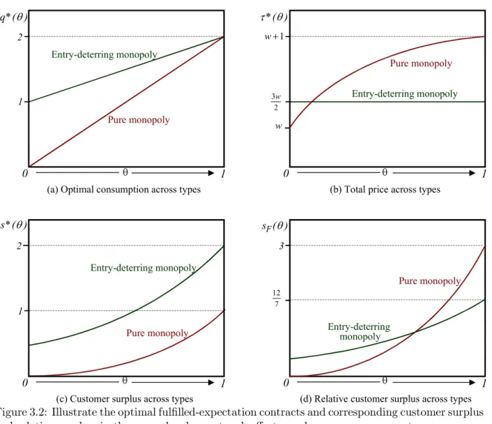
The contracts and surplus values that result from applying Propositions 1 and 2, and equations (3.6) and (3.7) are summarized in Table 3.1. Under pure monopoly, consistent with Proposition 1, consumption is unaffected by the network effects, and prices increase by an amount equal to the network value. Under entry deterring monopoly, individual consumption increases for all customers, and a fixed fee equal to the network value is charged to each customer.
q*( )q
q
0 1
1 2
(a) Optimal consumption across types Pure monopoly Entry-deterring monopoly *( ) t q q 0 1
(b) Total price across types Pure monopoly Entry-deterring monopoly 3 2 w 1 w+ w s*( )q q 0 1 1
(c) Customer surplus across types Pure monopoly Entry-deterring monopoly F s ( )q q 0 1 3
(d) Relative customer surplus across types Pure monopoly Entry-deterring monopoly 12 7 2
Figure 3.2: Illustrate the optimal fulfilled-expectation contracts and corresponding customer surplus and relative surplus, in the example when network effects are homogeneous across types.
τ∗(θ), one can derive the explicit pricing functionp(q) =q−q42, which is strictly concave, which in turn implies a progressively increasing quantity discount.
Under entry-deterring monopoly, prices increase for a subset of lower types. However, so does customer surplus, as indicated in Figure 3.2 (c). Furthermore, Figure 3.2 (d) shows that when there is a threat of entry, the relative distribution of surplus across different customer types is less skewed in favor of higher-usage customers. This is despite the increase in total price for the lower-usage customers, relative to the higher-usage customers.
4. Heterogeneous network e
ff
ects
This section models network effects that depend on both gross consumption and individual con-sumption. Both pure monopoly and entry-deterring monopoly are analyzed. The value function W(q,θ, Q) is assumed to be linearly separable in intrinsic value and network value, and to take the following form
W(q,θ, Q) =U(q,θ) +qw(Q).
4.1. Pure monopoly pricing
In the absence of an entry threat, the following proposition establishes the main characteristics of the optimal fulfilled-expectations contracts:
Proposition 3. (a) IfW(q,θ, Q) =U(q,θ) +qw(Q), then any optimal fulfilled-expectations con-tract satisfies the following conditions:
U1(q∗(θ),θ) +w(Q∗) U12(q∗(θ),θ) = 1−F(θ) f(θ) , (4.1) and τ∗(θ) =U(q∗(θ),θ) +q∗(θ)w(Q∗)− θ Z θ U2(q∗(x), x)dx, (4.2) whereQ∗ = θ R θ q∗(θ)f(θ)dθ.
(b) If w(Q)has a finite upper bound w, then an optimal fulfilled-expectations contract always
exists. In addition, ifw1(Q) <−U11(q,θ) for allQ and q,then (4.1) and (4.2) specify the unique
optimal fulfilled-expectations contract.
(c)For all θ,q∗(θ)> q0(θ), andτ∗(θ)>τ0(θ).
Sufficient conditions for the existence of an optimal fulfilled-expectations equilibrium are fairly mild — all that is required is that the marginal benefit from the network effects w(Q) be bounded. The condition for uniqueness requires that in general, marginal network value not grow too fast relative to marginal intrinsic value. However, even if the solution is not unique, this is not unduly troubling, since multiple possible equilibrium outcomes are not uncommon in models of network goods. The monopolist simply needs to pick the optimal fulfilled-expectations contract that provides the highest profits9. It is important to note that the results in part (c) of the proposition (and those in Proposition 5)do not rely on uniqueness.
0 1 q (q ) 2 12 2 2 1 ( ) ( , ) ( ) F U q f - q q q 1 12 1 1 1 ( ) ( , ) ( ) F U q f - q q q * 1( , )1 ( ) U qq +w Q 0 2 q (q ) * 1( , 2) ( ) U q q +w Q 1 * q (q ) q (* q2) 1 1 12 12 W ( q, ,Q ) U ( q, ) w( Q ) W ( q, ,Q ) U ( q, ) q = q + q = q
Figure 4.1: Illustrates the optimal consumption of two typesθ1andθ2(θ1<θ2) withheterogeneous network effects underpure monopoly. The marginal value curvesW1(q,θ, Q) are higher than the corresponding U1(q,θ) curves, by a constant amount w(Q). This results in a strict increase in consumption for all types, relative to the base case.
The network effects shift the customer value functions up by qw(Q∗) for all types. Since this shift is proportionate to individual consumption, it results in optimal quantities that are different from those of the base case. Part (c) of the proposition establishes that this is a strict increase for all types, and is illustrated in Figure 4.1, for two candidate types. Correspondingly, prices also go up for all customers. Sections 4.3 and 4.4 discuss the changes in the division of total surplus further.
4.2. Entry deterring monopoly pricing
The analysis of Proposition 3 is now extended to the case where a threat of entry is successfully deterred. Some new notation is introduced (though mostly in the proof of Proposition 4, which is in the appendix).
Let qm(θ, Q) denote the Q-optimal contract under pure monopoly. Applying Lemma 2, this allocation is defined for eachθby the necessary conditions
U1(qm(θ, Q),θ) +w(Q) U12(qm(θ, Q),θ)
= 1−F(θ)
f(θ) , (4.3)
fulfilled-expectations equilibrium — that is, there is a value of gross consumption such that Qm= θ Z θ qm(θ, Qm)f(θ)dθ. (4.4)
The following proposition establishes that the monopolist’s pricing scheme results in individual consumption that is either of the formqm(θ, Q), or that maximizesintrinsic value for the customer:
Proposition 4. Suppose W(q,θ, Q) = U(q,θ) +qw(Q). Assume that the uniqueness condition
w1(Q)<−U11(q,θ) from Proposition 3 is met. Define:
Qα = Q:qm(θ, Q) =α(θ),and (4.5)
ˆ
θ(Q) = θ:qm(θ, Q) =α(θ). (4.6)
(a) If Qα ≤Qm, then the unique optimal fulfilled-expectations contract is:
q∗(θ) = qm(θ, Qm) (4.7) τ∗(θ) = U(qm(θ),θ) +qm(θ)w(Qm)−U(α(θ),θ)−[ θ Z θ (U2(q∗(x), x)−U2(α(x), x))dx] (4.8)
(b) If Qα> Qm, then the unique optimal fulfilled-expectations contract is:
q∗(θ) = α(θ) (4.9) τ∗(θ) = α(θ)w(Q∗) (4.10) forθ≤ˆθ(Q∗),and q∗(θ) = qm(θ, Q∗) (4.11) τ∗(θ) = U(q∗(θ),θ) +q∗(θ)w(Q∗)−U(α(θ),θ)−[ θ Z ˆ θ(Q) (U2(q∗(x), x)−U2(α(x), x))dx](4.12)
forθ≥ˆθ(Q∗), whereQ∗ is the unique solution to:
Q= ˆ θZ(Q) θ α(θ)f(θ)dθ+ θ Z ˆ θ(Q) qm(θ, Q)f(θ)dθ. (4.13)
Proposition 4 establishes that the same conditions that ensure uniqueness of the optimal fulfi lled-expectations contract in the absence of an entry threat are sufficient to ensure uniqueness under the threat of entry. It also establishes that the optimal fulfilled-expectations contract that deters entry can be elegantly characterized using a combination of Q-optimal contracts under pure monopoly, and the contract that implements allocations of α(θ) for each typeθ.
If qm(θ, Qm) > α(θ) for the lowest type θ, an immediate corollary of the proposition is that the presence of the entry threat does not change the individual consumption of any of the types (since qm(θ, Qm) > α(θ) implies that Qα < Qm). This is likely to happen when the marginal network value w(Q) is high relative to marginal intrinsic value, or equivalently, if network effects are substantial for all types,. This is illustrated further in section 4.4.
Under the conditions of part (b) of the proposition, there are substantial changes in individual consumption (relative to pure monopoly). However, ˆθ(Q∗) is always an interior point of [θ,θ]. This implies that the larger increases in individual consumption (to the level α(θ) which maximizes intrinsic value) will always be for a subset of ‘lower’ types, and that there will always be a subset of higher types whose individual consumption is still of the form qm(θ, Q∗). It is easily shown that under part (b) of the proposition,Q∗ > Qm, which implies that consumption increases for all customer types (but more substantially for the lower subset).
4.3. Welfare analysis
This subsection characterizes how the monopolist and its customers share the surplus generated by the network effects under pure monopoly, and also discusses surplus division under entry-deterring monopoly.
Supposeq∗(θ),τ∗(θ) is an optimal fulfilled-expectations contract for some value functionW(q,θ, Q),
with realized gross consumption Q∗ = θ
R
θ
q∗(θ)f(θ)dθ. Relative to the base case, the net change in total surplus as a consequence of the network effects is therefore:
θ Z θ [W(q∗(θ),θ, Q∗)]f(θ)dθ− θ Z θ U(q0(θ),θ)f(θ)dθ. (4.14)
The direct change in surplus from a customer of type θas a consequence of the network effects is defined as:
sn(θ) =W(q0(θ),θ, Q0)−U(q0(θ),θ), (4.15)
where Q0 = Rθ θ
type θas a consequence of the network effects as
sq(θ) =W(q∗(θ),θ, Q∗)−W(q0(θ),θ, Q0) (4.16)
sn(θ) measures the change in surplus as a consequence of having the increase in value from the network effects, without accounting for any of the changes in consumption. sq(θ) measures the changes in surplus that arise indirectly as a consequence of the changes in consumption (both individual and gross) that the network effects induce. The total change in surplus across all types, as specified in (4.14), can now be equivalently expressed as
θ
R
θ
[sn(θ) +sq(θ)]f(θ)dθ.
Proposition 5. Under pure monopoly, the monopolist always captures all of the direct increase in surplus, and shares some of the indirect increase in surplus with the customers. That is:
θ Z θ τ∗(θ)f(θ)dθ− θ Z θ τ0(θ)f(θ)dθ≥ θ Z θ sn(θ)f(θ)dθ, (4.17) and θ Z θ τ∗(θ)f(θ)dθ− θ Z θ τ0(θ)f(θ)dθ< θ Z θ [sn(θ) +sq(θ)]f(θ)dθ, (4.18)
wheresn(θ) andsq(θ)are as defined in (4.15) and (4.16).
While proved for heterogeneous network effects, this result applies trivially to homogeneous net-work effects, since under Proposition 1, there is no indirect increase in surplus, and the monopolist captures all the direct surplus increase. Proposition 5 establishes that with heterogeneous network effects, the monopolist continues to get all the direct increase in surplus from the network effects, and that any increase in customer surplus are driven by increases in consumption.
Under entry-deterring monopoly, the division of direct and indirect increases in surplus is less relevant — all customers of type θget surplus at least equal to U(α(θ),θ), which implies that they capture all of the intrinsic value that they create. Moreover, the customer types whose optimal consumption is of the form qm(θ, Q∗) (that is, all customers under part (a), and the higher subset under part (b) of Proposition 4) capture a fraction of the network value that they create. Since U(α(θ),θ) > U(q∗(θ),θ) for q∗(θ) > α(θ), the monopolist needs to give up network value to the customer if they raise consumption beyondα(θ). The negative terms in square brackets at the end of equations (4.8) and (4.12) represent the surplus type θ gets beyond U(α(θ),θ), which implies that these customers are capturing a fraction over and above this reservation level.
Base case
Optimal contract: q0(θ) = 2θ;τ0(θ) = 2θ−θ2
Pure monopoly
Q-optimal contract: q(θ, Q) = 2θ+wQ,τ(θ, Q) = 2θ−θ2+wQ(2 +wQ)
2 Optimal fulfilled-expectations contract: q∗(θ) = 2θ+ w
1−w,τ ∗(θ) = 2θ−θ2+ w(2−w) 2(1−w)2 Surplus functions: s∗(θ) =θ(θ+ w 1−w), sF(θ) = 6θ(θ(1−w) +w) 2 +w
Table 4.1: Optimal contracts and surplus in theexamplewith heterogeneous network effects, under pure monopoly
4.4. Example
The example presented in Section 3.3 is extended to incorporate network effects that depend on individual consumption as well as on gross consumption. The value function is assumed to take the following form:
W(q,θ, Q) = (θ+ 1)q−1 2q
2+wqQ, (4.19)
and as before, customer types are assumed to be uniformly distributed between 0 and 1. The definitions of the surplus functions s∗(θ) and sF(θ) are in Section 3.3.
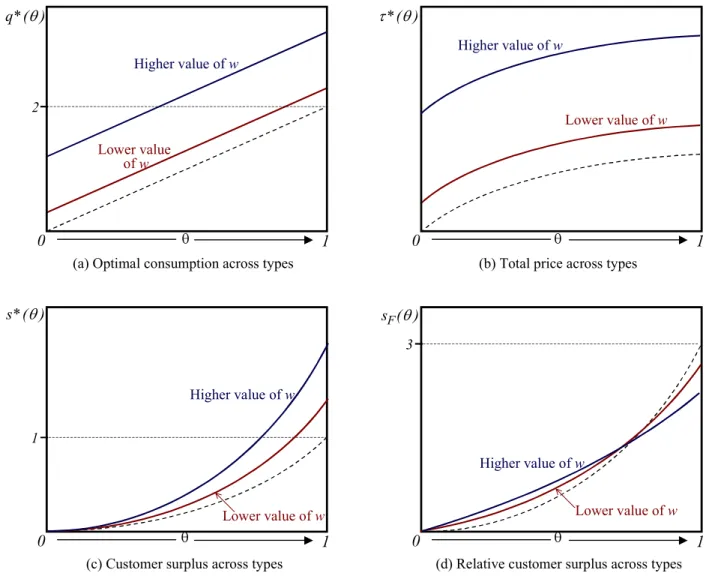
Since U11(q,θ) = −1, the uniqueness condition in Propositions 3 and 4 reduces to w < 1. Tables 4.1 and 4.2 summarizes the solutions for the optimal contracts and surplus functions under this condition. As expected from Proposition 3, both quantities and prices increase under pure monopoly, relative to the base case. Figure 4.2 (a) and (b) illustrate the optimal contract for two different values of marginal network valuew.In addition, by substitutingq∗(θ) intoτ∗(θ), one can obtain the explicit pricing function:
p(q) = w 2 4(1−w)2 + 2−w 2(1−w)q− q2 4 . (4.20)
The optimal pricing function is therefore a nonlinear two-part tariff, with a fixed component that increases with the marginal network valuew, and a strictly concave variable portion — again, implying a quantity discount that is progressively increasing. Moreover, differentiating (4.20) with respect to q indicates that p1(q) = 2(12−−ww) − q2, which is strictly increasing in w for w < 1. As a consequence, absolute prices at any level of consumption always increase withw.
As shown in Figure 4.2 (c), an increase inw increases customer surplus for all customer types. What is particularly interesting is that as w increases, the relative distribution of surplus across
q*( )q
q
0 1
2
(a) Optimal consumption across types Lower value of w *( ) t q q 0 1
(b) Total price across types s*( )q
q
0 1
1
(c) Customer surplus across types
F s ( )q
q
0 1
3
(d) Relative customer surplus across types Higher value of w Lower value of w Higher value of w Lower value of w Higher value of w Lower value of w Higher value of w
Figure 4.2: Illustrates the optimal fulfilled-expectation contracts and corresponding customer sur-plus and relative sursur-plus forpure monopoly, in the example when network effects are heterogeneous across types. In eachfigure, the dotted curve represents the base case (when network value is zero).
customer types is less convex. This is illustrated in Figure 4.2 (d), and indicates that at higher levels of network effects, surplus is distributed more evenly across customers of different types. This is a socially favorable result, because it suggests higher distributional equity of the value created, across customers who differ in their usage levels.
Under entry-deterring monopoly, equating the expressions for Qα and Qm indicate that part (a) of Proposition is applicable for w≥ 12, and part (b) applies forw≤ 12. This confirms that the entry threat induces changes in total surplus (via an induced change in optimal consumption) for lower levels of network effects, but not at higher levels.
As illustrated in Figure 4.3 (a), as w increases, optimal consumption is raised (relative to the corresponding levels under pure monopoly) for an increasingly smaller fraction of customer types, and when w ≥ 1, consumption is unaltered for all types (though total prices reduce by a fixed
Entry-deterring monopoly Intermediate variables: Qα= 1 w;Q m= 1 1−w; ˆθ(Q) = 1−wQ When w≥ 12
Optimal fulfilled-expectations contract: q∗(θ) = 2θ+ w 1−w, τ ∗(θ) = 1 2(1−w)2 −(1−θ) 2 Surplus functions: s∗(θ) =θ(θ+ w 1−w) + 1 2, sF(θ) = 3((2θ2+1)(1−w)+2θw) 5−2w When w≤ 12
Optimal fulfilled-expectations contract: θ≤ˆθ(Q∗): q∗(θ) =θ+ 1,τ∗(θ) =wQ∗(1 +θ)
θ≥ˆθ(Q∗): q∗(θ) = 2θ+wQ∗,τ∗(θ) = 2wQ∗−(1−θ)2 Surplus functions: θ≤ˆθ(Q∗): s∗(θ) = (1 +θ)2 2 , sF(θ) = 3(1 +θ)2 7 + (wQ∗)3 θ≥ˆθ(Q∗): s∗(θ) = (1+θ)2+(θ−2(1−wQ∗))2, sF(θ) = 3s ∗(θ) 7+(wQ∗)3 Note: When w≤ 12,Q∗ = 1− √ 1−3w2 w2 and ˆθ(Q∗) = w−1+√1−3w2 w
Table 4.2: Optimal contracts and surplus expressions in theexample with heterogeneous network effects, under entry-deterring monopoly
amount across all types).
At fairly low values of w, total price may increase for a subset of lower types. This is because the changes in consumption are substantial for these lower customer types, relative to the case of pure monopoly. Average prices (per unit of consumption) always decrease with a threat of entry, across all types. Clearly, customer surplus also increases, across all types.
Figure 4.3 (c) and (d) further highlight the socially desirable effect of a threat of entry that was noted in section 3.3 — the flattening of the relative distribution of surplus across types. This accentuates the increased distributional equity from increasing network effects that was illustrated in Figure 4.2(d). The former effect is more pronounced when network effects are lower. This is not surprising, since the latter effect is more pronounced when network effects are higher (and as a consequence, there is already less inequity across customers to begin with). This result has interesting policy implications, which are discussed further in Section 5.
5. Discussion
A number of new results relating to the pricing of network goods have been derived in Sections 3 and 4. This section discusses some of these results, examines some of the model’s assumptions, and
q
0 1
(c) Relative customer surplus across types (lower w) Entry-deterring
monopoly q*( )q
q
0 1
(a) Optimal consumption across types Lower value of w Higher value of w ˆ ( Q*) q *( ) t q q 0 1
(b) Total price across types Higher value of w ˆ ( Q*) q Lower value of w increasing w increasing w 3 F s ( )q q 0 1
(d) Relative customer surplus across types (higher w)
3 F s ( )q Pure monopoly Pure monopoly Entry-deterring monopoly
Fi gure 4.3: Illustrates the optimal fulfilled e x p ect at ion co ntr ac ts an d c or r es p on di ng re lat i ve cu s -tomer surplus forentry-deterring monopoly, in the example when network effects are heterogeneous. In eachfigure, the dotted curves represent the corresponding values in the case of pure monopoly.
concludes with an outline of open questions raised by the analysis.
5.1. Discussion of results
Managers in technology industries with network effects face especially difficult pricing problems. Their challenges include setting complex pricing schedules for variable quantity purchases, designing optimal quantity discounts, taking into account heterogeneity in network value across different customers, and also incorporating the reality that entry threats and ‘comparables’ from potential competitors play an important role in limiting the amount customers can be charged. Network effects pose an additional unique challenge, since there is the trade-off between designing prices that increase value from higher gross consumption, and prices that enables the seller to capture as
much of this value as possible.
This paper provide a set of theoretical results, based on a model which explicitly captures these issues, and can therefore form a robust basis for designing pricing policy for products of this kind. In addition, many empirical papers on network externalities (for instance, Gandal, 1995, Brynjolfsson and Kemerer, 1996, Forman, 2001) have studied technology markets — databases, spreadsheets, networking equipment — in which sellers with monopoly power routinely offer nonlinear pricing schedules, sell variable quantities to customers, and price to deter entry. The results of this paper could form a stronger theory base for future empirical work which aims to estimate the extent and implications of network effects in such markets.
When network effects do not vary across customers, Proposition 1 establishes that an increase in network effects induces no change in consumption, and that all surplus from the network effects is appropriated by the monopolist. A threat of entry changes pricing substantially — a fixed fee is offered to all customer types, and the outcome is socially optimal. While the specification of network effects in section 3 is simple, it would apply to industries in which the primary network value stems from a commonfixed-cost reduction — for instance, the cost offinding the appropriate hosting infrastructure, or qualified technical support. These results also indicate that if competing products are anything but perfectly compatible, any oligopoly outcome will be socially inferior to the entry-deterring monopoly outcome. In other words, from a regulatory perspective, ensuring a credible threat of entry is more socially efficient than actually inducing entry.
When the value realized from network effects varies with individual consumption, Proposition 3 establishes a strict increase in individual consumption across all customer types. In any model of nonlinear pricing, there is always a trade-off between value creation and price discrimination, and the consumption of lower customer types is limited by the monopolist’ desire to capture as much surplus as possible. The issue of value creation is accentuated further when there are network effects, since increases in consumption fromanysubset of customer types increases the value created byall customer types. The trade-offstill exists, though, and while pricing is redesigned to induce usage increases from both lower and higher customer types, the lower-usage customers still consume at a socially inefficient level. However, the relative distribution of surplus improves for lower customer types, implying that the network effects benefit lower-usage customers disproportionately, even though the higher-usage customers contribute relatively more to their actual magnitude.
Furthermore, when network value depends on individual consumption as well as gross con-sumption, the effects of an entry threat are less pronounced that those established by Proposition 2. In fact, as shown in Proposition 4(a), the threat of entry may have no effect on consumption or surplus, and may merely result in a price change that redistributes surplus between the monopolist
and its customers. Note that this occurs even when entry is not blockaded. This outcome is most likely when, relative to marginal intrinsic value, marginal network value is fairly high across all customers, as illustrated further by the example in Section 4.4.
The examples studied in sections 3.3 and 4.4 highlight the effect of network effects and entry deterrence on the relative distribution of surplus across participating customers. Regulatory agen-cies often consider implementing policy that affects not just total surplus, but the equity of surplus distribution across customers. For instance, the attention received by the issue of the ‘digital di-vide’ illustrates this potential objective clearly. Towards this end, this paper establishes that even if creating a credible threat of entry does not increase total surplus, it will reduce the inequity in surplus division across the different customers who generate the surplus through their consumption. In addition, there will always be accompanying transfer of surplus to all customers. While the outcome never maximizes total surplus, it is still likely that it is more efficient than an oligopoly with incompatible products.
5.2. Discussion of assumptions
The sequence of events specified in section 2.3 assumes that all customers have identical expectations of gross consumption. Under the assumption of rational participants, this is not restrictive — everyone has access to all the information needed to compute the expected consumption, and once the monopolist has specified prices, there is no residual uncertainty about demand. Clearly, in equilibrium, all customers must have the same expectation (the correct one).
However, compared to standard models of nonlinear pricing, this paper places a higher compu-tational burden on customers. Each customer has to knowF(θ), compute the optimal consumption (not just for themselves, but for all customer types), and them calculate the gross consumption. It may be likely that customers of network goods cannot actually compute the true gross consumption immediately, due to a lack of information, or due to bounds on information processing capability. There may be a multi-period adjustment process, in which customers iteratively make a series of guesses which converge to the fulfilled-expectations equilibrium outcome. Alternately, customers may learn the distribution of types from the pricing schedule. Formalizing these notions remains (early-stage) work in progress.
The assumption that W(q,θ, Q) has a finite maximum q for all θ and Q is non-standard. However, given that marginal costs are zero in the model, it is necessary in order to get a bounded solution. It is also a reflection of reality — that customers do stop using zero marginal price products at afinite level, typically due to the presence of resource constraints, and substitute uses for shared resources, as discussed in Section 2.1.
In addition, slightly modified versions ofall of the results in this paper continue to hold under the assumption of unbounded value functions and positive convex costs. Consider, for instance, a (standard) specification in which customer utility is ˜W(q,θ, Q), ˜W1(q,θ, Q) > 0 for all q (and
˜
W(q,θ, Q) has the other curvature properties attributed to the customer value function in this paper). In addition, suppose the provision of quantityq to each customer has a positive costc(q), wherec1(q)>0,c11(q)>0. If one defined the total surplus function as:
W(q,θ, Q) = ˜W(q,θ, Q)−c(q),
then W(q,θ, Q) would have the same properties as it does in this model. More importantly, all the expressions for q∗(θ) derived in the model would continue to be valid, and so would all the expressions forτ∗(θ), if it is treated as the optimal markup rather than the optimal price. In other words, the optimal contracts would beq∗(θ),(τ∗(θ) +c(q∗(θ))), with the same expressions forq∗(θ) and τ∗(θ) as derived in sections 3 and 4. Therefore, this paper’s results are also applicable for technology products that display positive network effects, but which have non-zero marginal costs (networking equipment or handheld computers, for instance)
Some of the paper’s results have specified conditions on the marginal network value that are necessary to guarantee uniqueness. However, none of the properties of the contracts derived in Propositions 1 through 3 depend on uniqueness, and neither do the results of Proposition 5. If there are multiple optimal fulfilled-expectations equilibria, all the monopolist needs to do is choose the one with the highest profits. Proposition 4 relies on uniqueness, though a slightly modified version holds if one assumes that the monopolist always chooses the highest-profit contract.
5.3. Concluding remarks
The value from network effects in this model vary across types due to the customers’ varying individual consumption needs. As formulated, the model does not yet admit differing network value across different types at thesame level of individual consumption. A model that incorporates this is work-in-progress. Early results suggest that for sufficiently heterogeneous marginal network value, network effects may harm low-usage customers. Related work-in-progress involves a setup where network value is of the form wF(Q) +qwV(Q). A more general characterization might be to model the network good as a multiproduct bundle, and characterize customers using a two-dimensional type vector, drawing on Armstrong (1996) and Rochet and Chone (1998). Admitting this extension is current work-in-progress.
Industries in which products display network effects are often natural monopolies, especially when competing products are incompatible and marginal costs are near-zero. Moreover,
entry-deterrence appears to play a significant role in practice (as illustrated by the Microsoft antitrust case). The analysis of entry-deterring monopoly is therefore likely to be very important for these industries. In light of the results obtained in this paper, a natural (and open) question that arises is how non-zero entry costs affects outcomes. Clearly, monopoly profits will increase, and entry deterrence will still be an optimal strategy — however, it is likely that profits will increase by less than the entry cost.
Finally, the analysis of entry deterrence suggests the feasibility of solving a general model of nonlinear pricing for competing network goods. If customers expect the competing products to have different levels of gross consumption, they would view them as vertically differentiated products, as in Stole (1995), which would admit pricing other than the zero-markup contracts in Mandy (1992). Similar issues have been analyzed in a model of coalition formation by Economides and Flyer (1998). Price reductions that increase network effects would become ‘quality’ investments, and the issue of how competitive intensity is affected by these investments becomes relevant, especially since Section 4.2 suggests that in a general model, the equilibrium profits of the smaller network are likely to be zero. Recent results from Rochet and Stole (2001) indicate the feasibility of modeling mixed-strategy equilibria, and I hope to address some of these questions in the near future.
References
1. Armstrong, M. “Multidimensional Price Screening.” EconometricaVol. 64 (1996), pp. 51-75.
2. Brynjolfsson, E., and Kemerer, C. “Network Externalities in Microcomputer Software: An Econometric Analysis of the Spreadsheet Market.” Management Science Vol. 42 (1996), pp. 1627-1647.
3. Cabral, L,. Salant, D., and Woroch, G. “Monopoly Pricing with Network Externalities.” International Journal of Industrial Organization Vol. 17 (1999), pp. 199-214.
4. Dewan, S. and Mendelson, H. “User Delay Costs and Internal Pricing for a Service Facility.” Management Science Vol. 36 (1990), pp. 1502-1517.
5. Economides, N. “Network Externalities, Complementarities and Invitations to Enter.” Euro-pean Journal of Political Economy Vol. 12 (1996a), pp. 211-233.
6. Economides, N. “The Economics of Networks.” International Journal of Industrial Organi-zation Vol. 14 (1996b), pp. 673-699.
7. Economides, N., and Flyer, F. “Technical Standards Coalitions for Network Goods.” Annales d’Economie et de Statistique Vol. 49/50 (1998), pp. 361-380.
8. Farrell, J. and Saloner, G. “Standardization, Compatibility, and Innovation.” Rand Journal of Economics Vol. 16 (1985), pp. 70-83.
9. Forman, C. “The Effects of Compatibility on Buyer Behavior in the Market for Computer Net-working Equipment.” Working Paper, 2001. Available at http://www.andrew.cmu.edu/˜cforman/
10. Fudenberg, D. and Tirole, J.Game Theory. Cambridge: MIT Press, 1991.
11. Fudenberg, D. and Tirole, J. “Pricing a Network Good to Deter Entry.” Journal of Industrial Economics, Vol. 48 (2000), pp. 373-390.
12. Gandal, N. “Competing Compatibility Standards and Network Externalities in the PC Soft-ware Market.” The Review of Economics and Statistics Vol. 77 (1995), pp. 599-608.
13. Jullien, B. “Participation Constraints in Adverse Selection Problems.” Journal of Economic Theory Vol. 93 (2000), pp. 1-47.
14. Jullien, B. “Competing in Network Industries: Divide and Conquer.” Working Paper, IDEI, University of Toulouse, 2001.
15. Katz, M. and Shapiro, C. “Network Externalities, Competition and Contracting.” American Economic Review Vol. 75 (1985), pp. 424-440.
16. Mandy, D. “Nonuniform Bertrand Competition.” Econometrica Vol. 60 (1992), pp. 1293-1330.
17. Maskin, E. and Riley, J. “Monopoly with Incomplete Information.” Rand Journal of Eco-nomics Vol. 15 (1984), pp. 171-196.
18. Mendelson, H. “Pricing Computer Services: Queuing Effects.” Communications of the ACM Vol. 28 (1985), pp. 312-321.
19. Mendelson, H. and Whang, S. “Optimal Incentive-Compatible Priority Pricing for theM/M/1 queue.” Operations Research Vol. 38 (1990), pp. 870-883.
20. Oren, S., Smith, S., and Wilson, R. “Nonlinear Pricing in Markets with Interdependent Demand.” Marketing Science Vol. 1 (1982), pp. 287-313.
21. Radner, R. “Equilibrium Under Uncertainty.” Chapter 20 in K. Arrow and M. Intriligator, eds., Handbook of Mathematical Economics Vol. 2. Amsterdam: North Holland Publishing Company, 1982.
22. Rochet, J., and Chone, P. “Ironing, Sweeping and Multidimensional Screening.” Economet-rica Vol. 66 (1998), pp. 783-826.
23. Rochet, J., and Stole, L. “Nonlinear Pricing with Random Participation.” forthcoming, Review of Economic Studies (2001).
24. Rohlfs, J. “A Theory of Interdependent Demand for a Communication Service.”Bell Journal of Economics Vol. 10 (1974), pp. 16-37.
25. Salani´e, B.The Economics of Contracts: A Primer. Cambridge: MIT Press, 1997.
26. Schmalensee, R. Written testimony, Civil Action No. 98-1232 United States versus Microsoft, 1999. Available at http://www.microsoft.com/presspass/trial/schmal/schmal.asp.
27. Segal, I., and Whinston, M. “Robust Predictions for Bilateral Contracting with Externali-ties.” Working Paper #0027, Center for the Study of Industrial Organization, Northwestern University, 2001.
28. Spence, A. M. “Entry, Capacity, Investment and Oligopolistic Pricing.” Bell Journal of Economics Vol. 8 (1977), pp. 534-547.
29. Stole, L. “Nonlinear Pricing and Oligopoly.” Journal of Economics and Management Strategy Vol. 4 (1995), pp. 529-562.
30. Sundararajan, A. “Nonlinear Pricing of Information Goods.” Working Paper #IS-02-01, Center for Digital Economy Research, New York University, 2002.
Available athttp://ssrn.com/abstract id=299337
A. Appendix: Proofs
Proof of Lemma 2
Given a expectation of gross consumptionQ, anyQ-feasible contractqF(t, Q),τF(t, Q) satisfies [IC] if:
θ= arg max t∈[θ,θ]
W(qF(t, Q),θ, Q)−τF(t, Q), (A.1)
for all θ. The necessary and sufficient conditions for (A.1) are:
[W1(qF(θ, Q),θ, Q)]q1F(θ, Q)−τF1(θ, Q) = 0∀θ; (A.2) [W11(qF(θ, Q),θ, Q)](qF1(θ, Q))2+ [W1(qF(θ, Q),θ, Q)]qF11(θ, Q)−τF11(θ, Q)≤0∀θ. (A.3) Differentiating (A.2) with respect toθand substituting (A.3) yields modified sufficient conditions:
[W12(qF(θ, Q),θ, Q)]q1F(θ, Q)≥0∀θ. (A.4)
By assumption, W12(q,θ, Q) is strictly positive, which means that (A.2) and (A.4) reduce to: τF1(θ, Q) = [W1(qF(θ, Q),θ, Q)]q1F(θ, Q), (A.5)
qF1(θ, Q) ≥ 0, (A.6)
for all θ.
Now, under the contract qF(t, Q),τF(t, Q), the surplus of typeθ is
s(θ) =W(qF(θ, Q),θ, Q)−τF(θ, Q). (A.7)
Differentiating (A.7) with respect toθ, and substituting (A.5) yields:
s1(θ) =W2(qF(θ, Q),θ, Q). (A.8)
Since reservation utility ˆU(θ) = 0 for all types, if IR is satisfied for the lowest typeθ, it is satisfied for all others. Therefore,s(θ) = 0, and
s(θ) = θ
Z
x=θ
Combining (A.7), and (A.9), the objective function whose maximizer is the optimal contract q(θ, Q),τ(θ, Q) can be written as:
θ Z θ=θ [W(qF(θ, Q),θ, Q)−{ θ Z x=θ W2(qF(x, Q), x, Q)dx}]f(θ)dθ. (A.10)
Integrating the second part of (A.10) by parts and rearranging yields:
q(θ, Q) = arg max qF(θ,Q) θ Z θ=θ [W(qF(θ, Q),θ, Q)−W2(qF(θ, Q),θ, Q) 1−F(θ) f(θ) ]f(θ)dθ, (A.11)
subject toq(θ, Q)≥0, and that
τ(θ, Q) =W(q(θ, Q),θ, Q)− θ
Z
x=θ
W2(q(x, Q), x, Q)dx. (A.12)
If the unconstrained problem has a unique solution for whichq(θ, Q)≥0, then this is the solution to the constrained problem as well.
Define
H(θ) = 1−F(θ)
f(θ) (A.13)
First-order conditions for the unconstrained problem are therefore:
W1(q(θ, Q),θ, Q) = [W12(q(θ, Q),θ, Q)]H(θ)∀θ, (A.14) and are sufficient if the point-wise profit function:
π(q,θ, Q) =W(q,θ, Q)−[W2(q,θ, Q)]H(θ) (A.15) is strictly concave inq. Differentiating (A.15) with respect toq twice yields:
π11(q,θ, Q) =W11(q,θ, Q)−[W112(q,θ, Q)]H(θ), (A.16) which verifies that π(q,θ, Q) is strictly concave, since W11 < 0, and W112 ≥ 0. This ensures that for the unconstrained problem,first-order conditions (A.14) yield the unique solution. These conditions can be rearranged as:
W1(q(θ, Q),θ, Q) W12(q(θ, Q),θ, Q)
= 1−F(θ)