ePub
WU
Institutional Repository
Doris Anita Oberdabernig
Revisiting the Effects of IMF Programs on Poverty and Inequality
Paper
Original Citation:
Oberdabernig, Doris Anita (2012) Revisiting the Effects of IMF Programs on Poverty and Inequality.
Department of Economics Working Paper Series, 144. WU Vienna University of Economics and
Business, Vienna.
This version is available at: http://epub.wu.ac.at/3609/
Available in ePubWU: August 2012
ePubWU, the institutional repository of the WU Vienna University of Economics and Business, is
provided by the University Library and the IT-Services. The aim is to enable open access to the scholarly output of the WU.
Department of Economics
Working Paper No. 144
Revisiting the Effects of IMF
Programs on Poverty and Inequality
Doris A. Oberdabernig
August 2012
Revisiting the Effects of IMF Programs
on Poverty and Inequality
∗Doris A. Oberdabernig† August, 2012
Abstract
Investigating how lending programs of the International Monetary Fund (IMF) af-fect poverty and inequality, we explicitly address model uncertainty. We control for endogenous selection into IMF programs using data on 86 low- and middle income countries for the 1982-2009 period and analyze program effects on various poverty and inequality measures. The results rely on averaging over 90 specifications of treatment effect models and indicate adverse short-run effects of IMF agreements on poverty and inequality for the whole sample, while for a 2000-2009 subsample the results are reversed. There is evidence that significant short-run effects might disappear in the long-run.
JEL codes: O11, O15, O19, C31.
Keywords: Poverty and income distribution, IMF lending programs, model uncer-tainty, treatment effects, cross-country analysis, developing countries
∗
The author would like to thank Jes´us Crespo-Cuaresma, Octavio Fern´andez-Amador, Joseph
Fran-cois, Elisabeth Nindl, Harald Oberhofer, Michael Pfaffermayr, Anna Raggl, Diego Romero de Avila Torrijos, Max Roser, Petra Sauer, Herbert Stocker, and three anonymous reviewers, as well as seminar participants at the wiiw Seminar in International Economics, and conference participants of the Annual International Conference on Macroeconomic Analysis and International Finance (ICMAIF, Greece), the Annual Meeting of the Austrian Economics Association (NOeG, Austria), the Applied Economics Meet-ing (EEA, Spain), the Macroeconometric Worskhop of the DIW Berlin (Germany), the Spanish Economic Association (SAEe, Spain), and the Workshop on The Political Economy of World Bank and IMF Aid at the Vienna University of Economics and Business (Austria) for helpful comments to earlier drafts of this paper.
†
Vienna University of Economics and Business, Department of Economics, Augasse 2-6, A-1090 Vienna, Austria, [email protected], Tel: +43(0)131336-4514, Fax: +43(0)131336-728
1
Introduction
At the end of World War II the international economic system was devastated. Certain rules and procedures were needed to recover economic stability and therefore the need for new institutions emerged. One of the institutions established in the course of the Bretton Woods Agreements in 1944 was the International Monetary Fund (IMF). It was assigned with regulating the international monetary and financial system and promoting its stability, encouraging economic cooperation, and helping to promote economic growth and the health of the world economy (IMF 2011a). As a result of the macroeconomic cries in Latin America and Africa the Fund joined the World Bank in providing sustained conditional lending to low-income countries in the mid-1980s and amplified its objectives with the one of poverty alleviation (Collier & Gunning 1999, IMF 2012a). The activity of the IMF is mainly implemented through arrangements between the IMF and a coun-try experiencing difficulties. Such an arrangement compromises a transfer from the IMF to the receptor country conditioned to some adjustment policies in order to promote a sustained growth path (IMF 2011b). Despite the efforts made by the IMF to reduce poverty, harsh criticism emerged that IMF programs lead to an increase in poverty in
re-cipient countries.1 This raised interest in answering the question whether IMF programs
contribute to reducing poverty, or, by contrast, if IMF critics are justified. In this study we apply a quantitative approach to clear that question and evaluate the effects of the IMF’s lending facilities on poverty rates and income distribution in participant countries. Although a big body of literature deals with analyzing the determinants of poverty and
income inequality, a unique theoretical framework is missing.2 This leads to the
inclu-sion of very heterogeneous sets of explanatory variables in different studies and empirical findings that are hardly unanimous in supporting a particular argument. One reason therefore might be the absence of universal causal mechanisms as there is no guarantee that the economic processes and its interactions with poverty and inequality are the same across countries or regions (Kenny & Williams, 2001). Due to data constraints research in this field of developing economics, however, usually relies on cross-country
or large-n panel-data evidence. Time series analyses that would give scope for more
detailed structural investigations are seldom possible. Hence, the findings of empirical work might be conditioned on the sample of countries (and the time period) covered by the study. But also the set of explanatory variables included in the regressions could drive the results.
Despite of the big number of regressors used in different studies it is common in the empirical literature to regress a usually small number of variables on poverty or income distribution, neglecting factors that have been proposed as determinants of poverty and inequality by other authors. This motivates the concern for taking into account model uncertainty, which is present in both the choice of explanatory variables and the result-ing estimates connected to it, in order to unveil universally applicable relationships that are not conditioned on a particular regressor set. As estimates obtained from selecting one model do not take uncertainty into account, the precision of the resulting coefficients is overestimated, thus, leading to a too confident interpretation of a variable as being
significant (Fern´andez et al. 2001).
1See Abugre 2000, Cavanaghet al. 2000, Hertz 2004, and Lundberg & Squire 2003.
2
For studies on the determinants of poverty see Adams (2004), Collier & Dollar (2002), Ghuraet al.
(2002), Morduch (1994), Mosleyet al. (2004), Nissanke & Thorbecke (2006), for inequality see Adams
To the knowledge of the author, Ghura et al. (2002) provide so far the only study that explicitly controls for model uncertainty in finding robust determinants of poverty. The work investigates the effect of 36 variables on average income in the lowest quintile of the income distribution in a Bayesian Averaging of Classical Estimates (BACE,
Sala-i-Martin et al. 2004) analysis. Six out of the 36 variables are identified as robustly
related to poverty—gross domestic product (GDP) per capita growth, inequality,
infla-tion, educational achievement, financial development, and government size—thus point-ing towards the universal applicability of their effects. In this study we aim to identify patterns concerning the impacts of program participation on poverty and inequality that are common to a big group of countries. To provide a comprehensive picture we look at six poverty indicators: The number of people living below the poverty line of 1.25$ or 2$ per day (headcount ratios), their income shortfall from these poverty lines (poverty
gaps), and income equality before and after redistribution (Gini indexes).3 As the focus
of this paper is to identify treatment effects, we take a slightly different approach to
Ghura et al. (2002). Instead of sampling over the whole model space (that is allowing
for every combination of explanatory variables) we restrict some of the variables to be included in each regression. We estimate 90 model specifications for each poverty indi-cator and perform model averaging over the results of the regressions. An explanation of the procedure can be found in Section 3.2.
The contribution of this study is twofold. On the one hand we provide an empirical study on a large group of countries (86 low- and middle income countries, from 1982 to 2009) taking both poverty and distributional aspects into account while controlling for endogenous selection into IMF programs. On the other hand we explicitly account for model uncertainty to work out to what extend this uncertainty puts the robustness of the effect of program participation under strain. This kind of robustness analysis about the consequences of IMF agreements for poverty and income inequality is the primary concern of this research rather than identifying robust determinants of those indicators. We find empirical evidence for adverse short-run effects of IMF agreements on the num-ber of people living in poverty, as well as on the severity of poverty (measured by the income shortfall from the poverty line). Income inequality (both, when measured before and after redistribution) is found to rise with program participation. Restricting the estimations to the 2000-2009 period the results are in many cases reversed.
The paper is structured as follows. Section 2 provides an overview of IMF programs, their theoretical implications for poverty and inequality, as well as a short review of the findings of more recent empirical studies. The estimation framework is outlined in Section 3. It describes the methodologies of treatment effect regressions and model averaging, followed by a summary of the model specifications. In Section 4 we report data-based analyses and regression results. Finally, Section 5 concludes.
2
IMF programs
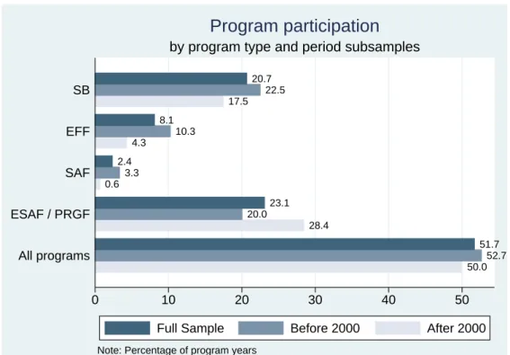
2.1 Types of IMF programs
This study addresses both concessional as well as non-concessional programs of IMF lending. Concessional loans carry zero interest payments (through the end of 2013) and
3Kanbur (1987) and Sen (1979) provide information about the construction of poverty indicators and
a discussion of their adequacy for measuring poverty. Concerning data quality, it is widely recognized that data on poverty and inequality suffer from measurement problems and comparability constraints. Deaton (2001) provides a summary about potential problems underlying the measurement of poverty. For an overview of caveats concerning inequality data see Atkinson & Brandolini (2001) and Solt (2009).
are available for low-income countries while non-concessional loans are subject to the
IMF’s market related interest rate, called the rate of charge4 (IMF 2012b). The
non-concessional loans we consider are provided through Stand-By Arrangements (SBA) and the Extended Fund Facility (EFF). SBAs are short-term agreements, which typically last from one to two years and imply higher conditionality than other types of IMF lend-ing programs. They are designed to help countries with severe disequilibria to respond quickly to their external financing needs. The greatest amount of IMF resources is pro-vided under SBAs. The EFF was established to help countries with severe disequilibria to address medium-term balance of payment problems which require fundamental eco-nomic reforms. The typical EFF program lasts for three years (IMF 2011c, and IMF 2011d). The three concessional programs that form part of this study are the Structural Adjustment Facility (SAF), which was established in 1986, the Enhanced Structural Adjustment Facility (ESAF) founded in 1987, and the Poverty Reduction and Growth Facility (PRGF), which replaced the ESAF in 1999. The SAF and the ESAF are longer-term programs with lower conditionality. Programs under the SAF normally imply less stringent conditionality than ESAF programs and mostly antecede ESAF programs. The PRGF is based on country-owned Poverty Reduction Strategy Papers, which are pre-pared by the government of the country concerned. The largest number of IMF loans
has been implemented through the PRGF in recent years (IMF 2011e, and IMF 2011f).5
The above mentioned lending facilities are connected to conditionalities. Conditionalities cover both policy requirements that a country has to fulfill in order that a tranche of the loan gets disbursed, as well as tools used to monitor progress towards the goal outlined in the program. These loan conditions should help to solve balance of payments problems
and ensure that the country will be able to repay the Fund (IMF 2011b). Typical
conditionalities include policies concerning trade liberalization, fiscal policy reforms and privatization, as well as financial reforms. These conditions affect poverty either directly
or as a channel for impacting on it.6
2.2 Theoretical impacts of IMF programs on poverty and inequality
Trade liberalization has two potential opposite effects on poverty. On the one hand, sectors that were protected before the liberalization contract, what leads to lower in-comes in these areas. On the other hand, according to the Stolper-Samuelson theorem, trade liberalization leads to increased demand and higher wages for unskilled workers in countries that are relatively abundant in unskilled labor (Handa & King 1997). Thus, the theoretical effect of trade liberalization on poverty ambiguous and depends on
pro-duction, trade, and consumption patterns (Gunter et al. 2005).7 Most of the work in
4
The rate of charge is based on the SDR interest rate, which is revised weekly to take account for changes in short-term interest rates in major international money markets.
5
As a reaction to the global financial crisis the IMF reshuffled the structure of lending facilities in 2009. The concessional lending facilities were rearranged and new non-concessional lending facilities emerged. The new concessional facilities include the Extended Credit Facility (ECF), which replaced the (PRGF), the Standby Credit Facility (SCF), and the Rapid Credit Facility (RCF), both replacing the Exogenous Shock Facility, which was established in 2008 (IMF 2011a, IMF 2011g). The Flexible Credit Line (FCL) and the Precautionary Credit Line (PCL) emerged in 2009 and 2010 respectively as new non-concessional lending facilities (IMF 2011h, and IMF 2011i). These recently created facilities, however, are not the focus of this study as it addresses IMF programs up to the end of the year 2009.
In the rest of the paper we will use the termsprograms and agreements for referring to IMF lending
programs.
6
For a theoretical overview of the effects of conditionalities on poverty see also Cashinet al. (2001).
For an overview about the results of empirical studies see Hajro & Joyce (2009).
7
Nissanke & Thorbecke (2006) provide a comprehensive overview about the channels through which globalization might affect poverty.
the recent empirical literature about the effects of trade liberalization on poverty shows that trade liberalization has a positive impact on poverty reduction, but leads to higher inequality. Looking at the effects of trade on inequality in more detail there is evidence that trade with high income countries worsens the income distribution of middle in-come countries while it has no effect on the inin-come distribution of low inin-come countries (Meschi & Vivarelli 2009).
A country under IMF agreement typically is obliged to decrease its budget deficit, which can be achieved through an augmentation of fiscal revenue or a decrease in public ex-penditure. The re-distributional effects of such reforms depend on the budgetary policy that the government implements. Usually reductions in public expenditure imply cuts in social spending, public sector wages, and public sector employment. The resulting rise in unemployment and the lower wages in this sector tend to increase poverty levels and worsen income distribution. Fiscal revenue can be increased with privatization of state-owned enterprises (mostly implying layoffs of public sector employees) or reform of the tax structure. Tax reform often implies a bigger focus on expenditure taxes and a simplification of income taxes and, therefore, leads to a deterioration of the after-tax
income distribution.8 There is no consensus in the literature concerning whether
partic-ipation in IMF programs results in a decrease in social expenditure.9
Financial reforms imply currency devaluation, liberalization of the financial sector, as well as an adjustment of the banking sector. Although there is no clear-cut conclusion
about the relationship between devaluation and poverty (Gunteret al. 2005),
devalua-tion is connected to negative associadevalua-tions in developing countries (such as increased costs of servicing foreign debt or capital flight of foreign investors). Theoretically, the effect of currency devaluation is a decrease in the price ratio of non-tradable to tradable goods which gives some scope for import substitution. Whether poor people benefit from a
devaluation depends on the composition of the economy and on consumption patterns.10
Financial liberalization is often connected to weaknesses in the domestic banking sector and currency crisis, leading to an increase in poverty. Therefore, such a liberalization needs to be accompanied by sound economic policies and legal and regulatory under-pinnings to improve economic performance (Bird & Rajan 2001). Bank reforms leading to higher interest rates or more restrictive bank-reserves requirements, as well as the introduction of credit ceilings, reduce the access to domestic credit and make it easier for large companies to get credits in contrast to small and medium-sized firms. Also, the urban sector is favored over the rural sector, resulting in rising inequality (Johnson & Salop 1980, cited by Vreeland 2002). Most of these fiscal and financial reforms (credit restraints, budgetary cuts, higher levels of taxation, and reductions in real wages) are very likely to reduce domestic demand. The resulting contraction of spending is most likely to decrease the welfare of people whose main source of income is labor income and people living in poverty (Heller 1988).
The policies implemented under IMF agreements should lead to a reduction of inflation and restore economic growth. Economists broadly agree that high levels of inflation have negative consequences on economic growth and poverty. Some studies, however, find that countries that maintain macroeconomic stability do not necessarily gain
sig-8
See Handa & King (1997), and Johnson & Salop (1980), cited by Vreeland (2002).
9See Handa & King (1997) and Nooruddin & Simmons (2006) for evidence that participation in IMF
programs leads to a decrease in social expenditure, and Martin & Segura-Ubiergo (2004) for evidence against it.
10
See Bourguignonet al. (1992), Garuda (2000), Kanbur (1987), and Pastor (1987) for more details
nificant improvements in economic growth and poverty reduction.11 Theoretically the effect of inflation on income distribution depends on how rigidly the income adjusts to prices for each group of the population. If poorer individuals face longer adjustment lags than wealthier people, a higher inflation rate will raise income inequality (Garuda, 2000). While it is not clear whether growth affects inequality in one way or the other, most authors agree that economic growth is fundamental for poverty reduction. Some point out that the sectoral composition of growth and its distributional effects matter for poverty alleviation. This highlights the need for appropriate politico-economic programs
that create conditions for the poor to benefit from growth.12 The empirical evidence
on whether participation in IMF programs leads to a higher rate of economic growth is ambiguous. Some studies find that IMF lending reduces economic growth, whereas
others find beneficial effects of IMF support on growth.13
The possibilities for implementing IMF programs are broad and imply different conse-quences for poverty and income distribution. Political power plays an important role in determining the design of the program and to which extent conditionalities are fulfilled. It is likely that IMF programs are carried out in a way that does not hurt politically powerful groups, frequently at the expense of the poor. Furthermore, participation in a program makes it easier for policymakers to tackle painful reforms as they can blame
the Fund for “forcing” them to do so.14
2.3 Empirical findings
Investigating the impacts of IMF agreements on the distribution of income most studies
find that program participation is connected to higher inequality. More recent large-n
studies that control for sample selection as opposed to many earlier investigations in this field include the work of Garuda (2000) and Vreeland (2002). While the study of Garuda suggests that IMF programs lead to a deterioration of the income distribution in countries with severe external imbalances but to a relative improvement in distributional indicators if imbalances are small, Vreeland concludes that program participation lowers the labor share of income in the manufacturing sector and thus contributes to rising inequality. In contrast to the study of Garuda that relies on propensity score group comparisons covering 39 countries over the 1975-1991 period, the work of Vreeland is based on a dynamic version of Heckman’s (1979) selection model for 110 countries over the 1961-1993 period. More recent studies that investigate the effects of program
partic-11
Easterly & Fischer (2001), Ghuraet al. (2002), and Meschi & Vivarelli (2009) agree on the negative
consequences of high levels of inflation, while Gunteret al. (2005) find no significant improvement in
economic growth and poverty reduction in periods of macroeconomic stability.
12Information about the effects of economic growth on inequality is provided by Deininger & Squire
(1998), Dollar & Kraay (2004), Ghuraet al. (2002), and Ravallion & Chen (1997). While Adams (2004),
Dollar & Kraay (2002), Fanta & Upadhyay (2008), and Ghuraet al. (2002) provide general evidence for
the effect of growth on poverty, Cashinet al. (2001), Garuda (2000), Hajro & Joyce (2009), Loayza &
Raddatz (2010), and Stiglitz (2002) point out that certain conditions have to be met in order for poor people to benefit from economic growth.
13
Atoyan & Conway (2006) point out the ambiguity of the effect of IMF lending on economic growth. For evidence that IMF lending reduces growth see Barro & Lee (2005), Bordo & Schwartz (2000), and Przeworski & Vreeland (2000), for evidence of the beneficial effects of IMF programs for growth see
Dicks-Mireaux et al. (2000), Evrensel (2002), and Hutchison (2004). Ul Haque & Kahn (1998) and
Steinwand & Stone (2008) provide a more detailed summary about the effects of participation in IMF programs on macroeconomic variables such as economic growth, inflation, balance of payments, and current account deficits.
14
Arpacet al. (2008), Garuda (2000), Pastor (1987), and Vreeland (2002) recognize that political power
plays a role both for program design and compliance with conditionalities. Collier & Dollar (2002), Dreher & Walter (2010) state that the IMF exerts a scapegoat function for implementing unpopular reforms.
ipation on poverty find that, both, IMF and World Bank programs lower the response of poverty levels to changes in economic growth (Easterly 2001). However, neither in-fant mortality nor the Human Development Index, as proxies for poverty, are found to be significantly different in countries that participate in an IMF agreement (Hajro & Joyce 2009). While the results of Easterlys’ work are based on instrumental variable regressions for 65 countries, the study of Hajro & Joyce does not explicitly control for
self-selection but performs fixed effects regressions for a sample of 82 countries.15
3
Estimation framework
In the empirical analysis we are confronted with several kinds of statistical challenges. First, there is a problem of unobservability of the counterfactual outcome. We can perceive what happens to countries that took part in an IMF agreement after program participation, but we cannot observe what would have happened to them otherwise. Sec-ond, we are confronted with an endogeneity problem, as the choice of a country whether to participate in a program is not made randomly. Countries which are more likely to join an IMF agreement generally face specific macroeconomic conditions that make them eligible for participation in programs (Przeworski & Vreeland 2000). These differences, which could themselves influence poverty and/or income distribution, have to be con-trolled for, otherwise leading to biased estimates of the effect of program participation. Finally, we also face a problem of model uncertainty, as it is not clear which factors are robust determinants of program participation and poverty indicators.
In order to address the first two issues and obtain unbiased estimates, we deal with program evaluation as a particular case of a treatment effects setup. Although it is impossible to observe the counterfactual outcome, the task is to match countries that participate in an IMF program with countries that face similar conditions but do not form part such a program. While some of these conditions are observable some, like po-litical will, might be not. Treatment effect regressions remove the effects of non-random selection taking into account both observable and unobservable factors. The remaining difference in poverty or inequality between countries that form part of IMF agreements
and countries that do not is the inherent effect of IMF programs (Vreeland 2002).16
In order to address model uncertainty, we estimate various treatment effect regressions with country fixed effects based on different sets of explanatory variables that could po-tentially be driving factors of program participation and poverty measures. We test for the presence of selection bias in each of the model specifications. If there is no evidence for such bias, we estimate OLS regressions with country fixed effects additionally to the treatment effect regressions. Based on the results we perform model averaging, placing more importance on models with higher explanatory power. For constructing the model weights, we use both Bayesian (Schwarz 1978) and frequentist (Akaike 1973) information criteria. Subsequently, we get an insight about which factors affect the poverty indica-tors used, independent of model specification and free of selection bias, and are able to evaluate the robustness of program effects.
15
For a summary of earlier research dealing with the effect of IMF programs on poverty and inequality see Hajro & Joyce (2009).
16
Vreeland (2003, pp. 112-116) provides a very good (intuitive) explanation of why it is important to take into account unobservables and how these characteristics are controlled for.
3.1 Treatment effects model
We are interested in estimating
yit=x0it−1β+δDit−τ+ξi+it (1)
whereyit is alternatively one of the six poverty indicators used in this study—the
natu-ral logarithm of poverty gaps and poverty headcount ratios both at the poverty line of 1.25$ and 2$ per day, and Gini indexes of gross and net income inequality—measured in
periodt for countryi,xit−1 is a vector of variables that likely affect poverty or income
inequality, and β is the corresponding parameter vector. Dit−τ is a dummy variable
which is equal to one if country iis participating in an IMF program at timet−τ and
zero otherwise.17 Its coefficientδ reports the effect of program participation on poverty
and income distribution. ξi is the time invariant country fixed effect of country i and
it is the random error term. As we cannot test for reverse causation due to data
lim-itations, all of the explanatory variables enter with one year time lag in order to avoid
contemporaneous feedback effects.18
Estimation results relying on specification (1) are potentially subject to bias due to en-dogenous selection into program participation, as countries do not make their choice whether to ask the IMF for help randomly but depending on their macroeconomic con-ditions and other (unobservable) factors. Therefore, it is not possible to tell if the effect on poverty or income inequality arises due to program participation or those differences,
unless controlling for non-random selection.19 To take this into account we make use of
treatment effect models, which allow to estimate the impact of program participation on poverty and income distribution consistently. Treatment effect models rely on an
instrumental variable approach in which the endogenous program participation Dit is
instrumented as
Dit∗ =wit0−1γ+zit0−1α+uit, (2)
and depends on a set of variableswit−1 which explain program participation, and at least
one exclusion restrictionzit−1, which should be correlated withDitbut uncorrelated with
yitin (1). The validity of the exclusion restriction is essential for effective bias correction.
γ and α are the coefficient vectors for these two sets of variables, and D∗it is a latent
variable with its observable counterpart Dit that is generated by
Dit =
1 if Dit∗ >0
0 otherwise
The system formed by (1) and (2) assumes bivariate normal distributed error termsuit
and it and homoscedasticity, withV ar(it) =σ2,V ar(uit) = 1, and Cov(it, uit) =ρσ,
and can either be estimated in two stages or jointly by maximum likelihood. Although computationally less expensive, the two stage estimator is inefficient compared to max-imum likelihood. Therefore, the latter approach is used in this paper (Heckman 1974,
Nelson 1984). As the treatment effects model accounts of endogeneity, δ is free of bias
17In the empirical section of the paperτ ranges from 0 to 2.
18
The same data limitations make us dependent on using cross country information for investigating the effects of IMF programs although the possibility exists that causal mechanisms differ across countries. By allowing for country fixed effects we take into account differences in levels of poverty and inequality.
19
See Conway (1994), Dreher & Walter (2010), Goldstein & Montiel (1986), Przeworski & Vreeland (2000), and Vreeland (2002).
and can be interpreted as the effect of program participation on poverty or income
dis-tribution, respectively.20
With this theoretical framework in mind, the researcher has to specify potential
determi-nants,x, of our poverty measures in equation (1)—what we will refer to as the outcome
equation—and the variables included inw and z that explain program participation in
equation (2)—what we will call the selection equation. The empirical literature on the determinants of participation in IMF programs proposes quite a lot of different sets of
explanatory variables driving such a decision.21 To the knowledge of the author, Sturm
et al. (2005) provide the first attempt to address model uncertainty including a very
broad set of explanatory variables which potentially influence the probability of
obtain-ing an IMF credit. Moser & Sturm (2011) update the work of Sturmet al. (2005) for the
post-Cold War period. Both studies make use of the Extreme Bounds Analysis proposed by Leamer (1983, 1985) and Levine & Renelt (1992) to identify robust determinants of IMF programs and analyze the entire distribution of the coefficient estimates as
pro-posed by Sala-i-Martin (1997). While Sturm et al. (2005) find that mostly economic
variables play a role in IMF lending decisions, Moser & Sturm (2011) suggest that also political variables matter.
Addressing model uncertainty in the selection equation (2) as outlined here, as well as in the outcome equation (1) as sketched out in Section 1, we estimate a broad range of alter-native models including different sets of regressors and instruments. Then, we perform averaging of the coefficients obtained from those model specifications using Bayesian and frequentist information for constructing model weights. The primary aim of applying this method is to ensure that a significant coefficient of the program dummy is not the result of model selection, but is robust to model specification.
3.2 Model averaging
The importance of sensitivity analyses for empirical studies has already been emphasized by Leamer (1983, 1985) who proposes a method for testing the robustness of variables, which he calls Extreme Bounds Analysis (EBA). EBA consists of running a battery of
regressions including variables that are common to each specification (free variables),
and additional explanatory variables (doubtful variables) that enter in any linear
com-bination in the model. In order to classify a variable as robust, the minimum and the
maximum of its coefficient have to be statistically significant and of the same sign. The EBA has been regarded to impose too strong conditions on the variable coefficients in order to be considered as robust, however, and new methods for dealing with model
uncertainty have developed (Fern´andez et al. 2001, Sala-i-Martin 1997, Sala-i-Martinet
al. 2004).
This paper builds on the Bayesian Averaging of Classical Estimates (BACE) proposed
by Sala-i-Martin et al. (2004), which relies on averaging ordinary least squares (OLS)
coefficients across models with model weights being proportional to the Bayesian
In-20For further details on treatment effect models consult Cameron & Trivedi (2009, pp. 869-871),
Greene (2008, pp. 889-890), Heckman (1978), or Maddala (2008, pp. 117-125).
21
Studies that deal with the participation decision in IMF programs include Andersenet al. (2006),
Atoyan & Conway (2006), Barro & Lee (2005), Bird & Rowlands (2001), Broz & Hawes (2006), Dreheret
al. (2009), Dreher & Walter (2010), Dreher & Sturm (2012), Eichengreenet al. (2008), Elekdag (2008),
Garuda (2000), Harriganet al. (2006), Moser & Sturm (2011), Przeworski & Vreeland (2000), Sturmet
formation Criterion, BIC (Schwarz, 1978). Applying model averaging in the context of program evaluation, the method we use differs from BACE in the way that we do not apply a sampling algorithm. Rather, we specify what Leamer (1985) calls free variables and sequentially include other variables which are believed to have an influence on the dependent variable. The resulting models form part of the averaging process. We pre-fer this approach to a full BACE approach because of two main aspects. In terms of variable selection we allow, on the one hand, only for model specifications which are theoretically reasonable, on the other hand, we can explicitly take care of the handling of exclusion restrictions, which we introduced in Section 3(a). Apart from that, in terms of efficiency, sampling over the whole model space would entail a huge computational expense, as Maximum Likelihood estimations of treatment effect models are rather time consuming.
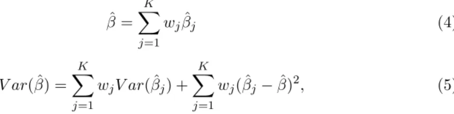
We follow Buckland et al. (1997) in using model weights which are obtained from
information criteria like the Akaike Information Criterion, AIC (Akaike, 1973), and the
BIC.22 The weight for modelkis calculated as
wk=
exp(−Ik/2)
PK
j=1exp(−Ij/2)
(3)
where I is the information criterion and K is the number of model specifications.
Fol-lowing Sala-i-Martinet al. (2004) we derive the model averaged coefficients, ˆβ, and their
variance, V ar( ˆβ), as ˆ β = K X j=1 wjβˆj (4) V ar( ˆβ) = K X j=1 wjV ar( ˆβj) + K X j=1 wj( ˆβj−βˆ)2, (5)
where ˆβj and V ar( ˆβj) are the coefficient and variance estimates from the treatment
effect regression with the regressor set that defines modelj.
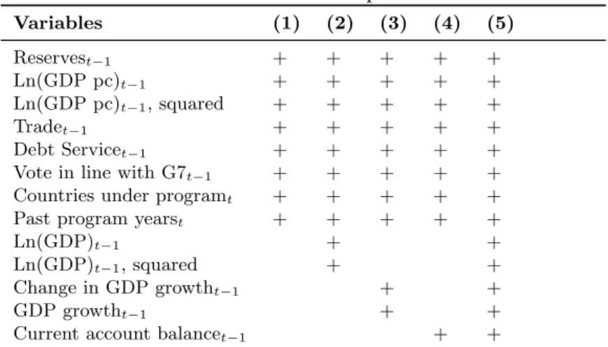
3.3 Model specifications
The results of this paper rely on averaging over 18 specifications of the outcome equa-tion (1), which are combined with five different specificaequa-tions of the selecequa-tion equaequa-tion (2). This leads to 90 treatment effect models being averaged for each poverty indicator. Table 1 shows the five specifications of the selection equation. The variables Vote in
line with G7t−1, Countries under programt, and Past program yearst serve as exclusion
restrictions,z.23 Appendix B discusses the model specifications in more detail and
pro-vides an overview of studies using the explanatory variables that are also included in
22
Raftery (1995) provides a formal derivation of the BIC approximation to the Bayes factor, the latter being used to construct model weights in a fully Bayesian context. Clyde (2000) gives a justification for model weights based on both the BIC and the AIC. The BIC is biased in favor of parsimony over fit while the AIC often tends to overestimate the number of parameters needed (Clyde 2000, Raftery 1995). Therefore, we perform model averaging with model weights based on either one of the two. The results based on the AIC, which are qualitatively the same as the ones obtained by the use of the BIC, are not reported here but are available from the author upon request.
23
Voting behavior in the UN General Assembly serves as a proxy for a country’s political proximity to the G7 countries who have some degree of influence over IMF decisions. Voting in line with G7 countries is found to be connected to a higher probability of obtaining a loan and better terms from the IMF. The number of countries under agreement in a certain year can be seen as a proxy for world conditions—as
the here presented work. Since the primary purpose of this paper is to investigate the effects of IMF programs on poverty and inequality, I refer to the studies mentioned in
the appendix for a discussion of the effect of the explanatory variables.24
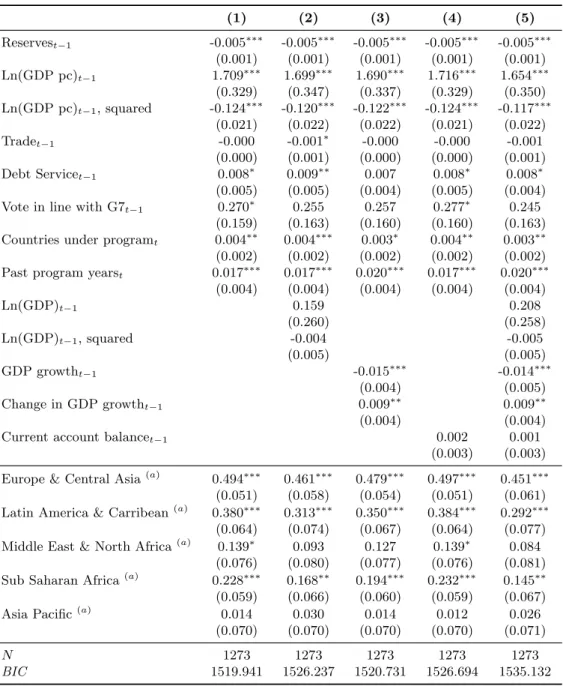
Table 1: Selection equations
Variables (1) (2) (3) (4) (5) Reservest−1 + + + + + Ln(GDP pc)t−1 + + + + + Ln(GDP pc)t−1, squared + + + + + Tradet−1 + + + + + Debt Servicet−1 + + + + +
Vote in line with G7t−1 + + + + +
Countries under programt + + + + +
Past program yearst + + + + +
Ln(GDP)t−1 + +
Ln(GDP)t−1, squared + +
Change in GDP growtht−1 + +
GDP growtht−1 + +
Current account balancet−1 + +
NOTE: + indicates that the variable is included in the specification.
Table 2 reports the 18 specifications of the outcome equation. A base of variables is included in each estimation which, additionally to variables proposed in the literature
like the logarithm of GDPper capita, a democracy index, and the Gini coefficient, also
includes country dummies and three time trends to control for common developments before participation in a program, during program participation and after the termina-tion of an agreement. The reason for the three exclusion restrictermina-tions to be included in all
specifications is to allow the assessment of their validity.25 We request at least one
exclu-sion restriction to be satisfied in order to use the estimation results for inference about program effects. The country dummies are included in order to control for individual effects that are time invariant. As shown in Table 2 each of the model specifications
adds different variables to the common base.26
world conditions are bad, more countries turn to the Fund. Alternatively, the more countries turn to the Fund, the less costly the sovereignty costs may be perceived to be, so more countries apply for a program
(Sturmet al. 2005). The number of years a country spent under IMF agreement is included because
countries that participated already in IMF programs are more likely to do so again. This happens as the political cost may be lower if a country has already participated in an IMF program before, as compared to the first agreement with the Fund (Vreeland 2003).
24
See Steinwand & Stone (2008) for a more complete survey about factors determining participation in IMF programs.
25Like already mentioned in Section 3(a), exclusion restrictions should be significant in explaining
the country’s participation decision in IMF programs but should not be correlated with the dependent variable of the outcome equation.
26
We drop individuals with less than two data points available. Note that the estimation of all model specifications is based on same number of observations (Akaike 1973, Schwarz 1978).
T able 2: Outcome equations V ariables (1 ) (2) (3) (4) (5) (6) (7) (8) (9) (10) (11) (12 ) (13) (14) (15) (16) (17) (18) Ln(GDP p c) t − 1 + + + + + + + + + + + + + + + + + + Demo cra cy index t − 1 + + + + + + + + + + + + + + + + + + Gini net t − 1 ( a ) + + + + + + + + + + + + + + + + + + Coun try dummies + + + + + + + + + + + + + + + + + + Y ears b efore program t , trend + + + + + + + + + + + + + + + + + + Program y ears t , trend + + + + + + + + + + + + + + + + + + Y ears after program t , trend + + + + + + + + + + + + + + + + + + Coun tries under program t + + + + + + + + + + + + + + + + + + P ast program y ears t + + + + + + + + + + + + + + + + + + V ote in line with G7 t − 1 + + + + + + + + + + + + + + + + + + Ln(GDP p c) t − 1 , squared + + GDP p c gro wth t − 1 + + + P opulation gro wth t − 1 + + Ln(In v estmen t)t − 1 + + + Ln(T rade) t − 1 + + + Ln(T rade) t − 1 , LIC + + + Ln(T rade) t − 1 , MIC + + + Exc hange rate gro wth t − 1 + + + > 200% depre ciation dumm yt − 1 ( b ) + + + Ln(Credit) t − 1 + + + Go v ernmen t consumption t − 1 + + + Ln(Inflation) t − 1 + + Deflation d umm yt − 1 ( c ) + + + Hyp erin flation dumm yt − 1 ( c ) + + + Natural resource ren tst − 1 + + + V alue added of agriculture t − 1 + + Urban p opulation t − 1 + + Y ears of sc ho oling t − 1 + + Life exp ectancy t − 1 + + Time tre nd t + + NOTE: + indicates tha t the v ariab le is included in the sp ecification. ( a ) The v a riable is only included in mo dels with p o v ert y gaps or headcoun t ratios as dep enden t v ariable. ( b ) W e add a dumm y for coun tries wit h dev aluations of more than 200% to con trol for outliers. ( c ) W e add dummies for deflation and h yp erinflation to b etter re presen t the coun tries in our sample.
Estimating the 90 treatment effect models for each of the six poverty indicators allows us to test for statistically significant error correlation between the residuals of the selection
equation and the ones from the outcome equation,ρσ(see Section 3(a)). A statistically
insignificant error correlation suggests that there is no endogeneity bias arising from endogenous selection of countries into a program and the equation could be estimated
by OLS. For these cases (where ρ turns out to be statistically insignificant) we also
estimate OLS regressions with country fixed effects. We include the same variables that form part of the selection and the outcome equation in the OLS regressions, leading to a maximum number of 90 model specifications also here. In order to gain insight on whether program participation affects poverty and income distribution upon impact, we
include the instrumented program participation dummy in the same year,t, in which the
poverty outcome is observed. Additionally, we estimate specifications in which program
participation is included with one (τ = 1), or two (τ = 2), time lags respectively. The
results are shown in Section 4.
4
Descriptives, results, and robustness
4.1 Data an descriptive statistics
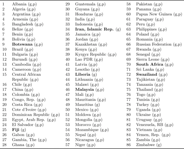
For investigating the effects of IMF programs empirically, we combine various databases to construct an (unbalanced) panel dataset which covers the period 1982-2009 and in-cludes 86 low- and middle income countries. Details about variables, data sources, and descriptive statistics concerning the variables used, as well as a list of countries included
in this study, can be found inAppendix A.
To provide a first, descriptive overview of the six poverty indicators that are the fo-cus of this study, we form five classes according to the program participation status of
countries. This leads to groups of countries which were never under IMF agreement
in the time period from 1982 to 2009, before the first program participation, currently
participating in a program, between two IMF programs and after the last IMF
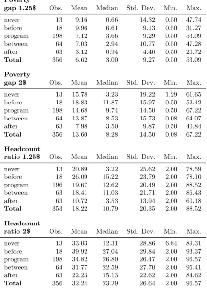
pro-gram that has been implemented in the country as long as data are reported. Table 3 provides summary statistics—number of observations, means, medians, standard devia-tions, minima, and maxima—for poverty gaps and headcount ratios. The distribution of all four indicators is positively skewed. Thus, focusing on the median values of the
indicators, poverty is the lowest for countries of our sample whichnever participated in
an IMF program, and the highest for countriesbefore their first participation and during
Table 3: Poverty gaps and headcount ratios by program participation status
Poverty
gap 1.25$ Obs. Mean Median Std. Dev. Min. Max.
never 13 9.16 0.66 14.32 0.50 47.74 before 18 9.96 6.61 9.13 0.50 31.27 program 198 7.12 3.66 9.29 0.50 53.09 between 64 7.03 2.94 10.77 0.50 47.28 after 63 3.12 0.94 4.40 0.50 20.72 Total 356 6.62 3.00 9.27 0.50 53.09 Poverty
gap 2$ Obs. Mean Median Std. Dev. Min. Max.
never 13 15.78 3.23 19.22 1.29 61.65 before 18 18.83 11.87 15.97 0.50 52.42 program 198 14.68 9.74 14.50 0.50 67.22 between 64 13.87 8.53 15.73 0.08 64.07 after 63 7.98 3.50 9.87 0.50 40.84 Total 356 13.60 8.28 14.50 0.08 67.22 Headcount
ratio 1.25$ Obs. Mean Median Std. Dev. Min. Max.
never 13 20.89 3.22 25.62 2.00 78.59 before 18 26.09 15.22 23.79 2.00 78.10 program 196 19.67 12.62 20.49 2.00 88.52 between 63 18.41 11.03 21.71 2.00 86.43 after 63 10.72 3.53 13.94 2.00 60.18 Total 353 18.22 10.79 20.35 2.00 88.52 Headcount
ratio 2$ Obs. Mean Median Std. Dev. Min. Max.
never 13 33.03 12.31 28.86 6.84 89.31 before 18 39.92 27.04 29.84 2.00 93.37 program 198 34.82 26.80 26.47 2.00 96.57 between 64 31.77 22.59 27.70 2.00 95.41 after 63 22.23 15.13 22.62 2.00 84.62 Total 356 32.24 23.29 26.64 2.00 96.57
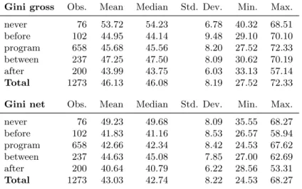
Table 4 shows summary statistics for Gini indexes of gross and net income inequality— the former measuring income inequality before taxes and transfers, the latter income inequality after redistribution. Both indexes are the highest for countries that never adopted an IMF program, indicating higher income inequality in those countries. They are the lowest after the last program participation.
Table 4: Gini indexes by program participation status
Gini gross Obs. Mean Median Std. Dev. Min. Max.
never 76 53.72 54.23 6.78 40.32 68.51 before 102 44.95 44.14 9.48 29.10 70.10 program 658 45.68 45.56 8.20 27.52 72.33 between 237 47.25 47.50 8.09 30.62 70.19 after 200 43.99 43.75 6.03 33.13 57.14 Total 1273 46.13 46.08 8.19 27.52 72.33
Gini net Obs. Mean Median Std. Dev. Min. Max.
never 76 49.23 49.68 8.09 35.55 68.27 before 102 41.83 41.16 8.53 26.57 58.94 program 658 42.66 42.34 8.42 24.53 67.62 between 237 44.63 45.08 7.85 27.00 62.69 after 200 40.64 40.79 6.22 28.56 53.31 Total 1273 43.03 42.74 8.22 24.53 68.27 4.2 Empirical specification
For illustrative purposes, coming to the specifications of the treatment effects models, Table 5 shows the results of probit estimations of the selection equations. It reports marginal effects at the means of the variables. In our sample most of the regressors turn out to be significant predictors of participation in an IMF programs with their coefficients
showing the expected sign. The natural logarithm of GDPper capita is found to have a
significant non-linear relationship with IMF program participation.27 The probability of
receiving an IMF program initially increases with GDP per capita but later decreases.
The estimated coefficients imply that the switch occurs at a GDP per capita between
$983.5 (column 1) and $1187 (column 2)28, which lies below the sample mean and the
sample median of the datasets used. The natural logarithm of GDP and its square, as well as the current account balance, turn out to be insignificant in predicting program participation. Voting behavior in the UN General Assembly and trade are only weak determinants of the adoption of an IMF agreement for the countries in our dataset. A possible reason for the insignificant or significantly negative trade coefficient in our sample is the lack of controlling for the composition of trade, for which unfortunately there are not data available.
27Ln(GDP pc) and its square are jointly significant with a p-value of 0.000 for each of the five
speci-fications. The same is true for ln(GDP) and its square, where the p-values for the joint significance lie between 0.0157 (specification 2) and 0.0261 (specification 5), respectively. When dropping the squared terms from the specifications, the coefficients of ln(GDP pc) and ln(GDP) turn out to be negative and significant, each. The results that are reported in Table 6 and Table 7 are robust to this specification change.
28
Table 5: Selection equations - Estimation (1) (2) (3) (4) (5) Reservest−1 -0.005∗∗∗ -0.005∗∗∗ -0.005∗∗∗ -0.005∗∗∗ -0.005∗∗∗ (0.001) (0.001) (0.001) (0.001) (0.001) Ln(GDP pc)t−1 1.709∗∗∗ 1.699∗∗∗ 1.690∗∗∗ 1.716∗∗∗ 1.654∗∗∗ (0.329) (0.347) (0.337) (0.329) (0.350) Ln(GDP pc)t−1, squared -0.124∗∗∗ -0.120∗∗∗ -0.122∗∗∗ -0.124∗∗∗ -0.117∗∗∗ (0.021) (0.022) (0.022) (0.021) (0.022) Tradet−1 -0.000 -0.001∗ -0.000 -0.000 -0.001 (0.000) (0.001) (0.000) (0.000) (0.001) Debt Servicet−1 0.008∗ 0.009∗∗ 0.007 0.008∗ 0.008∗ (0.005) (0.005) (0.004) (0.005) (0.004)
Vote in line with G7t−1 0.270∗ 0.255 0.257 0.277∗ 0.245
(0.159) (0.163) (0.160) (0.160) (0.163)
Countries under programt 0.004∗∗ 0.004∗∗∗ 0.003∗ 0.004∗∗ 0.003∗∗
(0.002) (0.002) (0.002) (0.002) (0.002)
Past program yearst 0.017∗∗∗ 0.017∗∗∗ 0.020∗∗∗ 0.017∗∗∗ 0.020∗∗∗
(0.004) (0.004) (0.004) (0.004) (0.004) Ln(GDP)t−1 0.159 0.208 (0.260) (0.258) Ln(GDP)t−1, squared -0.004 -0.005 (0.005) (0.005) GDP growtht−1 -0.015∗∗∗ -0.014∗∗∗ (0.004) (0.005) Change in GDP growtht−1 0.009∗∗ 0.009∗∗ (0.004) (0.004)
Current account balancet−1 0.002 0.001
(0.003) (0.003)
Europe & Central Asia(a) 0.494∗∗∗
0.461∗∗∗ 0.479∗∗∗ 0.497∗∗∗ 0.451∗∗∗
(0.051) (0.058) (0.054) (0.051) (0.061)
Latin America & Carribean(a) 0.380∗∗∗
0.313∗∗∗ 0.350∗∗∗ 0.384∗∗∗ 0.292∗∗∗
(0.064) (0.074) (0.067) (0.064) (0.077)
Middle East & North Africa(a) 0.139∗ 0.093 0.127 0.139∗ 0.084
(0.076) (0.080) (0.077) (0.076) (0.081)
Sub Saharan Africa(a) 0.228∗∗∗ 0.168∗∗ 0.194∗∗∗ 0.232∗∗∗ 0.145∗∗
(0.059) (0.066) (0.060) (0.059) (0.067)
Asia Pacific(a) 0.014 0.030 0.014 0.012 0.026
(0.070) (0.070) (0.070) (0.070) (0.071)
N 1273 1273 1273 1273 1273
BIC 1519.941 1526.237 1520.731 1526.694 1535.132
NOTE: Probit estimations. Dependent variable: Program participation dummy.
Marginal effects; Standard errors in parentheses. *** p<0.01, ** p<0.05, * p<0.1.
(a)
for discrete change of dummy variable from 0 to 1.
We do not show the estimation results of each of the treatment effects models as this would go beyond the scope of this paper due to space limitations. Rather we provide the results of the averaging across all models in the next subsection.
4.3 Averaging results and robustness
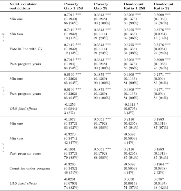
Table 6 reports the results of the averaging over the model specifications described ear-lier, for poverty gaps and headcount ratios as dependent variables. Because of space constraints we report only the results that are based on the BIC for constructing model
weights.29 Which poverty indicator has been used as the dependent variable is visible
29
in the head of the table. The table provides information about the contemporaneous
program effect on the poverty indicator (seen in the panel labeled τ = 0), as well as
program effects of one (τ = 1), or two years time lag (τ = 2). For which time lag the
results are reported can be seen in the first column. The second column indicates, for each time lag, how many and which exclusion restrictions have been satisfied in order to include a model in the averaging process. Also the results of the averaging over OLS fixed effects regressions (which were performed only for models where no selection bias was detected) are reported. Finally, the outcome of the averaging process can be found in the cells of the last four columns. Each cell reports the mean of the posterior distribution of the program participation coefficient with the significance level attached to it, as well as the posterior standard error (in parentheses) below. The number of model specifications included in the averaging process is reported at the bottom of each cell. In the case of treatment effects, it is the number of models (out of the 90 models estimated) which fulfill the respective exclusion restriction. In the case of fixed effects, it is the number of models for which no endogeneity bias was detected. The
percent-age in parentheses next to it indicates its fraction of the overall 90 model specifications.30
Table 6 reveals a clear-cut impact of program participation on poverty gaps and head-count ratios, measured at the poverty lines of 1.25$ and 2$ per day for our sample. As already mentioned, the results shown in the table rely on averaging the coefficients over different treatment effect regressions with country fixed effects (the values in the rows
labeled OLS fixed effects are an exception).31 According to the treatment effect results,
program participation turns out to increase both, the number of people living in poverty (poverty headcount ratios), as well as their income shortfall from the respective poverty line (poverty gaps). All poverty indicators worsen in the year the program is in force
(τ = 0), as well as in the following year (τ = 1). Two years after program
participa-tion has been observed, the undesirable effect of participaparticipa-tion in an agreement on most
poverty measures vanishes (τ = 2). Generally, the poverty augmenting effect of program
participation is stronger when poverty is measured at the lower poverty line of 1.25$ per day, meaning that the poorest members of the economy are hit the most by unfavorable program effects. Quantifying the effects, according to our data program participation has the biggest contemporaneous impact on the income shortfall of poor people from the 1.25$ poverty line followed by the number of people living below an income below this poverty line. The effects of IMF programs on the two poverty indicators measured
at the 2$ poverty line, are somewhat smaller.32 The magnitudes of the program effects
on poverty should be taken with care, however, as the measurement of poverty is not without problems (Deaton 2001). For most indicators the detrimental effect on poverty diminishes as we include more time lags between program participation and the poverty
index, until the program effect becomes insignificant.33 Turning to the OLS fixed effects
30
The high values of the percentages (for one fulfilled exclusion restriction) indicate that the reported outcome relies on a big number of averaged models and is not the result of only a few model specifications.
31
Like pointed out in Section 3(a), treatment effect regressions control for differences in economic conditions in countries prior to their participation in an IMF program and selection bias arising from it. As OLS regressions are just computed for model specifications for which treatment effect regressions
show an insignificant error correlation of the residuals,ρσ, the results relying on OLS fixed effects should
not be influenced by selection bias to a big extent.
32
The results suggest that the income shortfall from the 1.25$ poverty line more than doubles due to program participation, the shortfall from the 2$ line rises by up to 44%. The number of people living below the 1.25$ line increases by about 68%, or up to 39% considering the higher poverty line. Recall that
for obtaining these numbers the program coefficient has to be transformed as %∆y= [exp(δ)−1]×100.
33
One exception is the income shortfall of people from the poverty line of 2$ per day, which is found to be stronger affected as we increase the time between program participation and its impact on poverty. The effect of program participation (included with two years time lag) on this indicator remains
signifi-Table 6: Model averaging results - poverty indicators
Valid exculsion Poverty Poverty Headcount Headcount
restrictions Gap 1.25$ Gap 2$ Ratio 1.25$ Ratio 2$
τ = 0 0.7015 *** 0.3343 *** 0.5208 *** 0.3099 *** Min one (0.1940) (0.1248) (0.1373) (0.1065) 86 (96%) 90 (100%) 88 (98%) 87 (97%) 0.7419 *** 0.3643 *** 0.5225 *** 0.3276 *** Min two (0.1932) (0.1114) (0.1335) (0.0964) 10 (11%) 21 (23%) 32 (36%) 13 (14%) 0.7419 *** 0.3643 *** 0.5225 *** 0.3276 ***
Vote in line with G7 (0.1932) (0.1114) (0.1335) (0.0964)
12 (13%) 21 (23%) 34 (38%) 22 (24%)
0.7015 *** 0.3343 *** 0.5208 *** 0.3099 ***
Past program years (0.194) (0.1248) (0.1373) (0.1065)
84 (93%) 90 (100%) 86 (96%) 78 (87%) τ = 1 0.6190 *** 0.4875 *** 0.4309 *** 0.2571 *** Min one (0.2262) (0.1369) (0.1133) (0.094) 85 (94%) 90 (100%) 81 (90%) 85 (94%) 0.6190 *** 0.4875 *** 0.4309 *** 0.2571 ***
Past program years (0.2262) (0.1369) (0.1133) (0.094)
85 (94%) 90 (100%) 81 (90%) 85 (94%)
-0.1256 -0.1313 *
OLS fixed effects (0.0844) (0.0705)
3 (3%) 3 (3%) τ = 2 -0.1872 0.5051 *** 0.2116 0.1883 Min one (0.3372) (0.1792) (0.4205) (0.1319) 83 (92%) 88 (98%) 85 (94%) 87 (97%) -0.3270 -0.5026 Min two (0.3474) (0.5609) 42 (47%) 4 (4%) -0.1861 0.5051 *** 0.2116 0.1883
Past program years (0.3372) (0.1792) (0.4205) (0.1319)
79 (88%) 88 (98%) 85 (94%) 85 (94%)
-0.3266 -0.5026 0.1964 **
Countries under program (0.3432) (0.5609) (0.0848)
46 (51%) 4 (4%) 2 (2%)
-0.0201 0.0050 0.0787
OLS fixed effects (0.0793) (0.0614) (0.0497)
74 (82%) 51 (57%) 38 (42%)
NOTE: Averaged coefficient estimates of program participation, based on BIC.
*** p<0.01, ** p<0.05, * p<0.1. Averaged standard errors in parentheses.
Number of averaged model specifications below, percentage of total in parentheses.
regressions the averaging leads to statistically insignificant effects of program participa-tion in almost all of the cases. The only excepparticipa-tion is the favorable slightly significant effect of program participation on the number of people living in poverty (measured at
the lower poverty line of 1.25$ per day).34
cant only when the averaging is based on a small number of specifications (2% of total).
34
This finding should be treated with caution, however, as it relies on a relatively small number of model specifications (3% of total) for which sample selection bias has not been detected. In the other 97% of model specifications for this indicator, sample selection bias has been found to be present. For contemporaneous effects of program participation selection bias has been detected in each specification, therefore no OLS fixed effects results are reported.
Due to space constraints, we do not show the averaged coefficients of the other variables
forming part of the regressions but summarize the results here shortly.35 In line with
theory and previous studies, higher GDPper capita, as well as a higher level of
democ-racy, and a more equal distribution of income are found to significantly lower poverty
as measured by our four poverty indicators.36 The time trends indicate that poverty
increases in the time the program is in force.37 In some cases, the number of countries
that are participating in an IMF program in a certain year, which could serve as a proxy for world conditions (Vreeland 2002), turns out to be significantly correlated to higher poverty, measured at the 2$ per day poverty line. Including the natural logarithm of
GDP per capita squared, we find an interesting pattern. Its coefficient is found to be
positive and significant in explaining 1.25$ line poverty indicators (the coefficient of ln
GDPper capitabecomes more negative), while it is negative and significant in explaining
the 2$ line poverty indicators (the coefficient of ln GDPper capita becomes insignificant
or positive). This result suggests that as the level of per capita income increases, its
marginal impact on poverty at the 1.25$ line decreases, while the poverty reducing effect for poverty measured at the 2$ line becomes stronger. Other factors that are found to be significantly lowering poverty include domestic credit to the private sector (as sug-gested by Morduch 1994), which mostly affects poverty measured at the poverty line of
2$ per day, and currency devaluation (Gunteret al. 2005, and Kanbur 1987). A hyper
devaluation, however, (measured as a devaluation of more than 200% within one year) is found to lead to an increase in poverty. There is also some, but limited, evidence that a higher average in years of schooling, higher life expectancy, and urbanization are significantly correlated to lower poverty rates, while hyperinflation leads to a rise in
poverty.38 The data suggest that the general development over time has been a decrease
in poverty.39 Variables whose effect on poverty remains unclear are trade openness and
population growth. Their coefficients are insignificant in most cases and, if significant, the direction depends on the specification of the estimation. Investment, government
consumption, GDP per capita growth, a country’s natural resource rents, and the value
added in agriculture are not found to be significant determinants of poverty.40
Providing further details,Appendix C gives an overview about the treatment effect
mod-els that enter with the highest weights in the averaging process. For each poverty and income inequality indicator it reports the estimation results of the tree “best” model
specifications, where program participation enters without time lag in the model.41
35In the following we denote a variable as having an effect on poverty if it is statistically significant at
least at the 10% level.
36These results are in line with Adams (2004), Fanta & Upadhyay (2008), Ghuraet al. (2002), Mosley
et al. (2004), and Nissanke & Thorbecke (2006). As opposed to our findings Ghuraet al. (2002) did not find democratic institutions being a robust determinant of the income share of the lowest quintile.
37
There is slight evidence that the number of people living with less than two dollars per day has been increasing before program participation and has been decreasing afterwards. This, however, cannot be confirmed for other poverty indicators.
38
The findings concerning education and life expectancy are in line with Easterly & Fischer (2001),
Fanta & Upadhyay (2008), Ghura et al. (2002), and Nissanke & Thorbecke (2006). Theoretically
however, higher urbanization is suggested to lead to an increase in inequality, and therefore also results in higher poverty (see Kuznets 1955, and Nissanke & Thorbecke 2006), what cannot be confirmed by this study.
39
This finding is in line with Mosleyet al. (2004) and Ravallion & Chen (1997).
40Ghura et al. (2002) identify GDPper capita growth as a robust determinant of poverty, what is
opposed to our result.
41Due to space constraints we report only the results for contemporaneous program participation. The
results for the inclusion of program participation with one or two years time lag can be obtained from the author upon request.
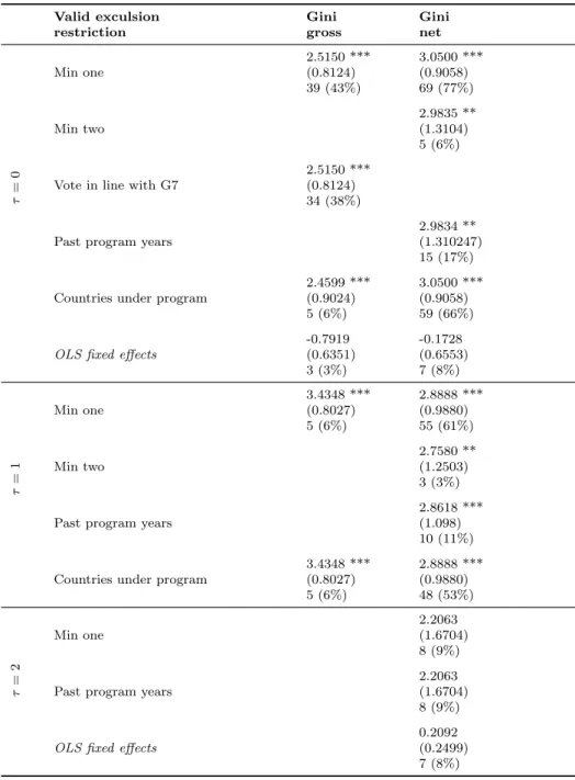
Table 7: Model averaging results - income inequality indicators
Valid exculsion Gini Gini
restriction gross net
τ = 0 2.5150 *** 3.0500 *** Min one (0.8124) (0.9058) 39 (43%) 69 (77%) 2.9835 ** Min two (1.3104) 5 (6%) 2.5150 ***
Vote in line with G7 (0.8124)
34 (38%)
2.9834 **
Past program years (1.310247)
15 (17%)
2.4599 *** 3.0500 ***
Countries under program (0.9024) (0.9058)
5 (6%) 59 (66%)
-0.7919 -0.1728
OLS fixed effects (0.6351) (0.6553)
3 (3%) 7 (8%) τ = 1 3.4348 *** 2.8888 *** Min one (0.8027) (0.9880) 5 (6%) 55 (61%) 2.7580 ** Min two (1.2503) 3 (3%) 2.8618 ***
Past program years (1.098)
10 (11%)
3.4348 *** 2.8888 ***
Countries under program (0.8027) (0.9880)
5 (6%) 48 (53%) τ = 2 2.2063 Min one (1.6704) 8 (9%) 2.2063
Past program years (1.6704)
8 (9%) 0.2092
OLS fixed effects (0.2499)
7 (8%)
NOTE: Averaged coefficient estimates of program participation, based on BIC.
*** p<0.01, ** p<0.05, * p<0.1. Averaged standard errors in parentheses.
Number of averaged model specifications below, percentage of total in parentheses.
Table 7 is built up in a similar way to Table 6 and shows how IMF programs affect income inequality in our sample. The results based on treatment effect regressions indicate that program participation is connected to higher income inequality measured both before
redistribution (Gini gross), and afterwards (Gini net).42 While program participation
42
The results here rely on a smaller number of model specifications because for many specifications none of the three exclusion restrictions is fulfilled. Especially, when the time lag with which program participation is included in the regressions is increased, less exclusion restrictions satisfy the requirement of being significant in the selection equation but insignificant in the outcome equation. Estimating the ef-fect of two years lagged program participation on the income distribution measured before redistribution, none of the exclusion restriction is valid for any of the model specifications.
seems to have a stronger contemporaneous effect on income inequality after taxes and transfers, the reverse is true if the program dummy enters the estimations with one year time lag. The increase in the Gini indicators as a result of program participation lies between 2.5 and 3.5 points. The same caution as before in interpreting magnitudes also applies here. Including program participation with two years time lag, the significant effect of IMF programs disappears. Averaging over the OLS fixed effects estimations (for model specifications for which no sample selection bias is detected) reveals a statis-tically insignificant effect of IMF programs on income inequality. Our results support the findings of Vreeland (2002) who finds a deterioration of income equality due to a decline in the labor share of income resulting from the adoption of IMF programs. Concerning the effect of other variables we find evidence for an equalizing effect of higher levels of democracy and a bigger amount of years a country has spent under IMF
program, while countries with higher per capita GDP and countries that vote in line
with the G7 are connected to a higher degree of inequality. According to these results a higher average income leads to both, a reduction in poverty, and a deterioration in income
inequality. Hence, an increase in GDPper capita does not translate into a proportional
rise in the income of the poor, as opposed to what is sometimes assumed in the literature (Collier & Dollar 2002). We find that inequality before taxes and redistribution is rising in program years, while both indicators are rising after program participation. There is some limited evidence that before program participation inequality has been decreasing. For our sample we can confirm Kuznets’ (1955) hypothesis that inequality is increasing
with income, but as a certain income per capita is attained the income distribution
becomes more egalitarian. Furthermore, the data reveal strong evidence that higher levels of investment and domestic credit to the private sector as well as higher life expectancy are correlated with higher inequality. As those indicators, among others, can be seen as reflecting the development status of a country, the income gap seems to widen as countries become more developed. Thus, in the context of Kuznets’s (1955) hypothesis, the countries in our sample did not yet reach the state of development
beyond which the income distribution becomes more equal. Notwithstanding, ceteris
paribus, the general development in our sample is a decrease in inequality over time.
Apart from that, we find that higher openness to trade is associated with a greater
degree of inequality,43 in contrast to currency depreciation and deflation, which are
connected to a more equal income distribution.44 Finally, there is some limited evidence
that higher rates of population growth and government consumption are connected to
higher inequality (Ghura et al. 2002, Kuznets 1955), while a bigger value added in
the agricultural sector, higher growth of GDP per capita, and a higher average level of
education lead to a decline in inequality.45
4.4 Have things changed after 2000?
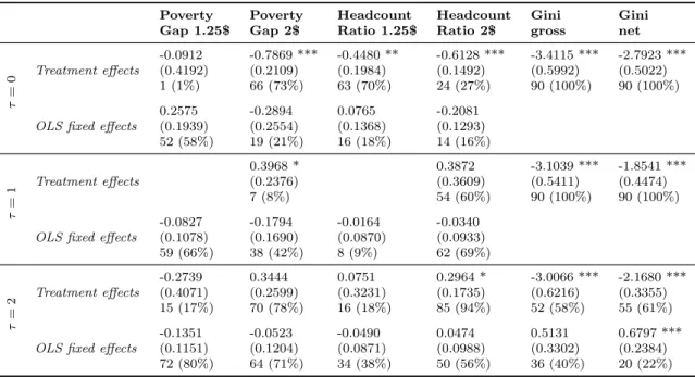
It can be argued that with the introduction of the PRGF in 1999 bigger focus was paid to the reduction of poverty and inequality. Therefore we estimate the same equations for the 2000-2009 period. Table 8 summarizes the results of the model averaged estimations
43
In comparison to Meschi & Vivarelli (2009) we lack data to control for the origin of imports and the destination of exports to take into account the development status of the trading partner. Meschi & Vivarelli (2009) find that trade with industrialized countries worsens the income distribution of middle income countries, while trade with other developing countries leads to an improvement.
44
Meschi & Vivarelli (2009) find a deterioration in income equality due to high levels of inflation.
45
These results are in line with Kuznets (1955), Nissanke & Thorbecke (2006), and Ravallion & Chen (1997).