Poly-GAN: A Multi-Conditioned GAN for Multiple Tasks

(1)

Rochester Institute of Technology Rochester Institute of Technology

RIT Scholar Works

Theses

12-2019

Poly-GAN: A Multi-Conditioned GAN for Multiple Tasks

Nilesh Pandey [email protected]

Follow this and additional works at: https://scholarworks.rit.edu/theses

Recommended Citation Recommended Citation

Pandey, Nilesh, "Poly-GAN: A Multi-Conditioned GAN for Multiple Tasks" (2019). Thesis. Rochester Institute of Technology. Accessed from

This Thesis is brought to you for free and open access by RIT Scholar Works. It has been accepted for inclusion in Theses by an authorized administrator of RIT Scholar Works. For more information, please contact

(2)

Poly-GAN: A Multi-Conditioned GAN

for Multiple Tasks

(3)

Poly-GAN: A Multi-Conditioned GAN

for Multiple Tasks

Nilesh Pandey

December 2019

A Thesis Submitted in Partial Fulfillment

of the Requirements for the Degree of Master of Science

in

Computer Engineering

(4)

Poly-GAN: A Multi-Conditioned GAN

for Multiple Tasks

Nilesh Pandey

Committee Approval:

Dr. Andreas Savakis Advisor Date

Dr. Raymond Ptucha Date

(5)

Acknowledgments

I would like to express my sincere gratitude to Dr. Andreas Savakis for his con-tinuous support and for believing in my ideas related to research. Dr. Savakis always motivated us to achieve new heights by letting us think freely. Under the supervision of Dr. Savakis, I improved not only as a researcher but also has an employee. I am very thankful for his guidance and support throughout my master’s program in the computer engineering department.

I would also like to thank my colleagues from Vision and Image Processing Lab; Dr. Breton Minnehan, Bhavan Vasu, Aman Arora, Navya Nagananda, Abu Md Niamul Taufique, Bryan Blakeslee, Bruno Miranda. Throughout my research on different topics related to my thesis, Discussion and arguments lead to new ideas after another.

I would also like to thank Professor Dr. Raymond Ptucha, who motivated me to research Computer Vision and Deep Learning, and for his constant support and guidance throughout my master’s program.

Finally, I owe everything to my father Umesh Pandey and my mother Rekha Pandey, who are there for me at every step in my life, giving me the utmost freedom to make decisions in my life.

I would also like to thank my friends for entertaining my ideas and giving their approval.

(6)

I would like to dedicate this thesis to my beloved parents, Umesh and Rekha Pandey for their eternal love and support.

(7)

Abstract

We present Poly-GAN, a novel conditional GAN architecture that is motivated by different Image generation and manipulation applications like Fashion Synthesis, an application where garments are automatically placed on images of human models at an arbitrary pose, image inpainting, an application where we try to recover a damaged image using the edges or a rough sketch of the image. While different applications use different GAN setup for image generation, we propose only one architecture for multi-ple applications with little to no change in the pipeline. Poly-GAN allows conditioning on multiple inputs and is suitable for many different tasks. Our novel architecture enforces the conditions at all layers of the encoder and utilizes skip connections from the coarse layers of the encoder to the respective layers of the decoder. Coarse lay-ers are easier to manipulate in shape change using condition, which results in higher level change in the result. Our system achieves state-of-the-art quantitative results on Fashion Synthesis based on the Structural Similarity Index metric and Inception Score metric using the DeepFashion dataset. For the image inpainting task we are achieving competitive results compared to current state of the art methods.

(8)

3.3.2 Poly-GAN Architecture . . . 43 3.3.3 Discriminator . . . 46 3.3.4 Loss Function . . . 46 3.4 Experiments . . . 47 3.4.1 Training Methodology . . . 47 3.4.2 Dataset . . . 48 3.4.3 Quantitative Evaluation . . . 49 3.4.4 Qualitative Evaluation . . . 50 3.5 Conclusion . . . 53 4 Discussion 54 Bibliography 56

(10)

List of Figures

1.1 GAN setup with Generator and Discriminator. . . 4

1.2 Result of mode collapse. [1] . . . 5

1.3 Progressive GAN setup with Generator and Discriminator. . . 7

1.4 Conditional Progressive GAN setup with Generator and Discriminator. 8 1.5 Conditional Progressive GAN result for label (1,1,1,1,1,1,1,1)x8. . . . 8

1.6 Conditional Progressive GAN result for label (2,2,3,4,9,6,1,2)x8. . . . 9

2.1 PhotoShop result from [2]. . . 12

2.2 Gated Convolution architecture. . . 13

2.3 SC-FEGAN architecture. . . 14

2.4 Image inpainting via Generative Multi-column Convolutional Neural Networks. . . 16

2.5 Poly-GAN: Generator network. . . 18

2.6 ResNet module. . . 19

2.7 Discriminator network. . . 21

2.8 Samples from the dataset LFW [3], CelebA [4], FFHQ. The green and purple lines represent the alignment of facial features across the dataset. 24 2.9 Results from Gated Convolution (Online Demo) . . . 25

2.10 Results from Generative Multi-column Convolutional Neural Networks (public release code). . . 26

2.11 Results from Generative Multi-column Convolutional Neural Networks (public release code). . . 27

2.12 Results from SC-FEGAN (publicly released demo). . . 28

2.13 Results from Poly-GAN edge based inpainting. . . 29

2.14 Results comparison of Generative Multi-column Convolutional Neural Networks [5], Gated Convolution [2] and edge based inpainting. . . . 30

2.15 Results from edges of reference based inpainting. . . 31

2.16 Results from rough sketch based inpainting. . . 33

2.17 Results from edge based inpainting. . . 34

2.18 Results from edge based inpainting. . . 35

3.1 Examples of Fashion Synthesis results generated with Poly-GAN. Shown in the columns from left to right: model image, reference garment, Poly-GAN result. . . 39

(11)

LIST OF FIGURES

3.2 Architecture of Virtual Try-On Network. . . 40 3.3 Poly-GAN pipeline. Stage 1: Garment transformation with Poly-GAN

conditioned on the RGB skeleton of the model and the reference gar-ment. Stage 2: Garment stitching with Poly-GAN conditioned on the segmented model, the RGB skeleton and the transformed garment. Stage 3: Refinement for hole filling with Poly-GAN conditioned on the stitched image and difference mask indicating missing regions. Stage 4: Postprocessing for combining the outputs of Stages 2 and 3 with the model head for the final result. . . 42 3.4 Poly-GAN architecture. The left side shows the encoder in green and

decoder in blue. The example shown is for garment transformation (Stage 1) but the architecture is the same for image stitching and inpainting. The conditions of reference garment and body pose are fed at all of the encoder layers. Skip connections from coarse layers of the encoder are fed to the corresponding layers of the decoder. The top right block shows the decoder module and the bottom right block shows the encoder module. . . 44 3.5 Architecture of the Discriminator. The example shown is for garment

transformation but the architecture is the same for image stitching (Stage 2) and inpainting (Stage 3). . . 44 3.6 Poly-GAN results shown from left to right column: Model image; Pose

Skeleton; Reference Garment; Stage 1: transformed garment; Stage 2: garment stitched on segmented model; Stage 3: refinement of outputs from stage 2: Stage 4: post-process result from stage 2 and stage 3 with head in original model image. . . 50 3.7 Poly-GAN results shown from left to right column: Model image; Pose

Skeleton; Reference Garment; Stage 1: transformed garment; Stage 2: garment stitched on segmented model; Stage 3: refinement of outputs from stage 2: Stage 4: post-process result from stage 2 and stage 3 with head in original model image. . . 51 3.8 Comparison examples of Poly-GAN with CP-VTON. Shown in columns

from left to right: model image, reference garment, CP-VTON result, Poly-GAN result. . . 52 3.9 Results of models randomly generated using StyleGAN. . . 52

(12)

List of Tables

2.1 Code and Demo link of the method used for comparison. Code in-dicates that we have used authors provided code for testing, Demo indicates that we have used authors provided demo for testing. . . 22 2.2 Methods are tested on randomly sampled images from the LFW dataset.

We test our edge based method against Generative Multi-column Con-volutional Neural Networks (GMCNN) and inpainting using Gated Convolution. Bold text in the above table shows best performance. . 30

3.1 Fashion Synthesis Quantitative Results. Bold numbers indicate best performance. . . 49

(13)

Chapter 1

Introduction

1.1 Motivation

The human brain has shown the most complex and sophisticated intelligence in the known universe. Throughout the evolution of humanity, artistic and creative designs demonstrate the brain’s capacity. We look for inspiration that can guide us or give us a more abstract idea of the end product in our inventions. For example, Leonardo da Vinci took inspiration from kites, spirals to create a modern prototype of the helicopter which could have worked given the design. Another such example involves developments in the fashion industry, where designers take their inspiration from day to day life to create fashionable garments. In the case of image painting, the algorithms take inspiration from the surrounding context and colors in the image. Artistic design is often inspired by something that the artists have already encountered in their experience. We believe AI can also greatly benefit from subtle hints like edges, skeleton, and color in images. In this thesis, we try to explore how hints, in the form of conditions, can benefit AI in creating subjects that they have never encountered before. We explore the phenomenon of using conditions with adversarial network in two applications a) Fashion Synthesis and b) Image Inpainting. The deep learning paradigm of Generative Adversarial Networks (GANs) has proven to be a suitable candidate for generating new images that are statistically close to the image samples

(14)

CHAPTER 1. INTRODUCTION

that are used for training.

The fashion industry has surged over the past few years because of e-commerce websites that let one shop for clothes or fashion garments from their comfort zone. The surge in demand to make the shopping experience as realistic as possible has led many researchers to invest their time in developing methods that can let people try clothes virtually as people do in a real shop. This virtual shopping attempt also tries to reduce the cost of logistics associated with people returning or exchanging the clothes that they buy online. It could also help in reducing the number of manufactured clothes, as the people would have the power to try many variations of clothes on a single click instead of the limited editions of the same design.

The other interesting application of image inpainting is based on the motivation to recover damaged images or edit images as per one’s wish. Image inpainting finds applications in tasks like doodling, image enhancement, and image editing. Image inpainting can be used in scenarios where one wants to remove an unwanted object or scene from the image. The other interesting application is to edit or enhance a portrait.

We believe that AI can be a one-stop solution to let people try clothes virtually or recover damaged images or edit the images as they wish. We hope to develop a network solution that can tackle multiple problems in the image generation task. Generative Adversarial Network (GAN) based methods are the state of the art net-works in image generation, image editing, and fashion synthesis. We believe we can deploy only one network architecture that it is capable of handling many image gen-eration tasks. We evaluate our developed methods on several datasets and compare them to state of the art methods.

(15)

Figure 1.1: GAN setup with Generator and Discriminator.

1.2 Generative Adversarial Networks

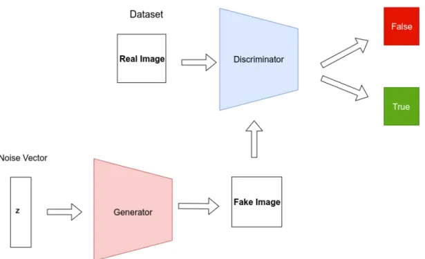
Generative Adversarial Networks [6] are very popular in various applications that require the creation of new data samples. GANs consist of two deep neural networks i.e the Generator and the Discriminator, as shown in Figure 1.1. The task of the Generator in the GAN is to generate new samples. The generated samples are con-sidered as fake samples, that do not necessarily resemble statistical closeness to the actual training data. The task of the Discriminator is to distinguish between the fake samples and the actual samples. The goal of the GAN setup is to have a min-max game between the Generator and the Discriminator. The Generator tries to minimize the error of fake samples, and the Discriminator maximizes the ability to distinguish between real and fake. The GAN setup tries to achieve Nash-equilibrium, where the Generator and the Discriminator no longer affect each other. The equation for min-max loss in GAN.

(16)

Figure 1.2: Result of mode collapse. [1]

.

min

G maxD V(D,G) =Ex∼pdata(x))[log(Dx)] +Ez∼pz(z))[log(1 −D(G(z)))] (1.1)

The simple architecture of the GAN setup is shown in Figure 1.1, where the Generator takes a random noise vector (Z) as input to generate data samples. The generated samples are passed to the Discriminator to decide whether the generated sample is a true sample from the dataset or fake sample. The training of GANs is an active topic of research because of a) Non-Convergence b) Mode Collapse, discussed next.

Mode Collapse In Figure 1.2, we have the results of generated MNIST samples from a GAN before and after mode collapse. In the MNIST dataset, we have ”0” to ”9” modes which represents 10 different classes. In the case of mode collapse, the network starts generating fewer classes more often, with no diversity in image generation.

(17)

1.3 Conditional Generative Adversarial Networks

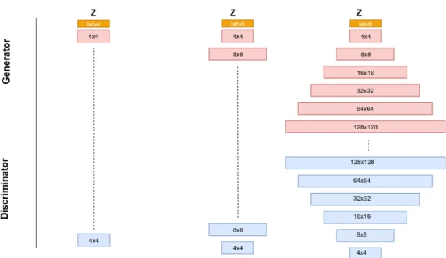
Conditional Generative Adversarial Networks (CGAN) [7] are a variant of GANs, that take a conditional input along with the actual input to the Generator. The setup of CGAN is similar to the original GAN setup, except for the input that now contains the noise vector. The noise vector with a condition could be a label or any other appropriate data input. Based on the concept of conditional GAN, we design our naive conditional progressive GAN shown in Figure 1.4

1.4 Progressive GAN

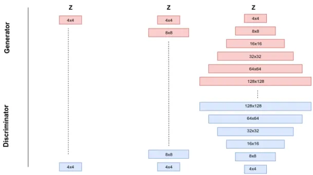
Generating high-resolution images is a difficult task in GANs due to the instability in training, and the mode collapse that can take place in the network. The authors of [8] suggest that while training the GAN setup, the layers of the Generator and the Discriminator should be increased one at a time to generate a high-resolution image. Progressively increasing layers in the Generator and the Discriminator results in stable training and a reduced chance of the mode collapse.

In Figure 1.3 initially a noise vector is given as an input to the Generator. The Generator consists of a layer capable of generating an image of size 4x4. The Discrim-inator is capable of distinguishing the generated image from the resized real image. The layers are progressively added to the Generator and the Discriminator once the training stabilizes on the current layer. The training procedure is stable since it is eas-ier to stabilize a network generating low-resolution images than directly attempting to stabilize a network generating high-resolution images.

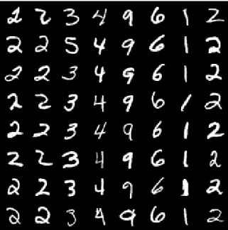
We make a version of progressive GAN shown in Figure 1.4 which is a conditional progressive GAN (CPGAN). The CPGAN is capable of generating data samples ac-cording to the labels we pass with the noise vector as the condition. In Figure 1.5 we pass label (1,1,1,1,1,1,1,1)x8 as a condition to the CPGAN, which is able to generate

(18)

Figure 1.3: Progressive GAN setup with Generator and Discriminator.

high-resolution Image. In Figure 1.6 we pass label (2,2,3,4,9,6,1,2)x8 as a condition to the CPGAN, which is able to generate high-resolution image. In some cases, we have a few missing generated classes.

(19)

Figure 1.4: Conditional Progressive GAN setup with Generator and Discriminator.

(20)

(21)

Chapter 2

Inpainting

2.1 Introduction

Recovering masked or damaged images and image editing are very popular, yet chal-lenging topics in computer vision. Photoshop, a widely popular tool used for image editing cannot always generate realistic images as seen in Figure 2.1 where the change or editing region is too large. Image recovery, the task of recovering masked images given a partial image, is a big challenge since there is no prior information on the subject. Image recovery can be tackled by extracting structural information like edges from the partially masked image or from a structurally similar image that can be used as a prior condition. Additionally, editing the edges of the partially destroyed region can be used as a prior condition.

Image inpainting for images with irregular damage is a challenging problem. The damage to the image could range from thin lines to large holes. Depending on the damage, one could try a different approach to the problem. If the damage is small, then it could be tackled using a classical computer vision algorithm, which will fill the gap using nearby pixel information. But if the damage is more than 20% of the image, then it is favorable to have a deep-learning approach. Methods like Partial convolution [9], Gated convolution [2] can generate realistic images subject to the availability of abundant training data and resources. The mentioned methods fail

(22)

CHAPTER 2. INPAINTING

when the image is too different from the training data or has some structure which the network has never seen before. This causes the generated image to be blurry or have visible artifacts.

In this chapter, we propose Poly-GAN, a conditional GAN architecture for image inpainting and Image editing. We perform subsequent experiments to show the sig-nificance of our proposed architecture. In our proposed conditional GAN, we pass the conditional input in every layer of the encoder while maintaining the relative statistics between the learned weights and the incoming conditional input. The main aim of the thesis is to generalize inpainting tasks for different applications including image inpainting and image editing that many recent state of the art methods are unable to perform. We believe that for a method to be useful in real-world applications, it should be able to generalize across the images which are different from the datasets they are trained on.

The main contributions of this thesis can be summarized as follows:

1. A generalized architecture for different inpainting applications, including image inpainting, image recovery and image editing.

2. A new conditional Generative Adversarial Network capable of handling many different and distinct tasks.

3. A method to edit and complete images based on edges or drawing information.

2.2 Related Work

Many different methods have been proposed for image inpainting. A very popular approach is the Patch-based image inpainting [10] network, which progressively learns to associate nearby features to the missing region, but fails in the free form image inpainting. The free form image inpainting poses a challenge of missing fine and distinct features from the nearby regions.

(23)

Figure 2.1: PhotoShop result from [2].

Traditionally, most of the inpainting papers focused on a damage region that is square or rectangular. Image Inpainting using Partial Convolution [9] is one of the first papers to show a free form of image inpainting on images with irregular damage. The paper utilizes a neural network with a new convolution layer called partial convolution with automatic update on the binary mask. Given a binary mask, the partial convolution utilizes non-damaged features in the nearby damaged region. The next step in the method is to update the binary mask according to the output of the partial convolution. If the output is positive for the damaged region then the mask is updated accordingly.

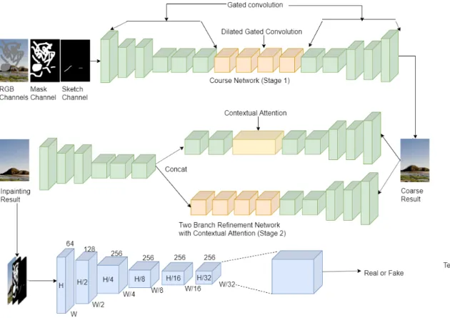
Free-form image inpainting with Gated Convolution [2] is another state-of-the-art method for inpainting images with irregular damage. This architecture, shown in Figure 2.2, introduces a new convolution layer named gated convolution. The input features in the model are first used to compute the gating value i.e., g = sigmoid(Wg ∗x), where x denotes the input features. The final output of the layer

is multiplication of learned features and gating values i.e., y = φ(W ∗x)g. The architecture includes a contextual attention module with the refinement network, with both having a gated convolution layer. Gated Convolution has inspired many of the newer state-of-art methods for image inpainting.

(24)

meth-CHAPTER 2. INPAINTING

(25)

Figure 2.3: SC-FEGAN architecture.

ods based on image editing. The work by providing the network a simple sketch of the face. Both papers have a similar approach to generating sketch images of the face, which can be edited and passed to the model as conditional input. Both models tend to use similar U-net style architecture for the Generator part.

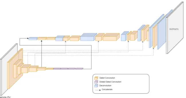
The SC-FEGAN network is shown in Figure 2.3. Its generator differs from Face-Shop by utilizing Gated Convolution and dilation convolution. The discriminator used in SC-FEGAN is similar to that proposed in [2] SN-patchGAN. The SC-FEGAN, shown in Figure 2.3, can train both the generator and the discriminator and can generate a high-resolution image (512x512). The generator in the SC-FEGAN setup has gated convolution in all layers followed by a Local Signal Normalization layer, as in [8], except the initial input layer in the encoder and final output layer in the decoder. The initial input layer to the encoder consisting of the damaged RGB image (3 channel), binary rough sketch (1 channel), RGB stroke map (3 channel), binary mask (1 channel), Gaussian noise (1 channel), i.e., 512x512x9 is the initial input to the encoder, which results in the output of 512x512x3 from the decoder of the Generator.

(26)

The loss function in FEGAN is discussed next. The final loss to train SC-FEGAN consists of total variational loss, style loss, perceptual loss, reconstruction loss, GAN loss as shown in Equations 2.1, 2.2, and 2.3. Icomp is the image

gener-ated from the generator, assuming that there is no destroyed region that is image completed, Igen is the image generated from the generator, θ is the feature map of

input when passed through some layer q of VGG16. Nx is the number of elements of

feature x. M is the binary mask. Gq =θq(X)Tθq(X) is the Gram matrix equation to

perform autocorrelation of features from the qth layer of VGG, and Cq is the number

of channels in the qth layer of VGG16.

LG SN =−E[D(Icomp)] (2.1)

LD =E[1−D(Igt)] +E[1 +D(Icomp)] +θLGP +E[D(Igt)2] (2.2)

LG =Lper−pixel+σLpercept+βLGSN +γ(Lstyle(Igen) +Lstyle(Icomp)) +υLtv (2.3)

Lper−pixel= 1 NIgt kM(Igen−Igt))k1 +α 1 NIgt k(1−M)(Igen−Igt))k1 (2.4) Lpercept= X q kΘq(Igen)−Θq(Igt)k1 Nθq(Igt)) + X q kΘq(Icomp)−Θq(Igt)k1 Nθq(Igt)) (2.5) Lstyle(I) = X q 1 CqCq k (Gq(I)−Gq(Igt)) Nq k1 (2.6)

(27)

Figure 2.4: Image inpainting via Generative Multi-column Convolutional Neural Net-works.

Ltv−col =

X

(i,j)∈R

kIcompi,j+1−Icompi,j k1

Ncomp (2.7)

Ltv−row =

X

(i,j)∈R

kIcompi+1,j−Icompi,j k1

Ncomp (2.8)

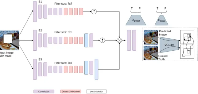
Image inpainting via Generative Multi-column Convolutional Neural Networks (GMCNN) is shown in Figure 2.4 [5]. The GMCNN network consists of 3 sub-networks, one of them is the Generator, 2 of them are the global and local discrimi-nator for adversarial training, and a pre-trained VGG network for the calculation of ID-MRF loss. Only the generator is deployed in case of testing of the image.

Another inpainting method is Implicit diversified Markov Random Field (ID-MRF) regularization. The idea behind ID-MRF is to reduce the distance between the generated content in the image and the corresponding nearest neighbor in the ground truth. We define the Loss for ID-MRF as follows,

RS(v, s) =exp(( µ(v, s)

max_rρ_v₍_YL₎µ(v, r)) +

(28)

In equation 2.9, YL _and _YL

G are target image features and generated image features

the from Lth layer of pre-trained VGG19, as shown in 2.4. The parameters h and

are constants, and µ is the cosine similarity function. The equation is normalized in 2.10. Finally the loss between YL _and _YL

G is defined in equation 2.11, where Z is

the normalization factor. The final MRF loss is computed using multiple layers in VGG19 as shown in equation 2.12.

The GMCNN approach [5] uses a spatial variant reconstruction loss other than the generic GAN loss, which is defined in equation 2.14, whereθ is a learnable parameter, M is the mask, and X is the input. G is the symbol for the Generator, and D is the symbol for the Discriminator.

RS(v, s) =RS(v, s)/ X rερv(YL) RS(v, r) (2.10) LM(L) =−log( 1 Z X sYL max vYˆL g RS(v, s)) (2.11) Lmrf =LM(conv4 2) + 4 X t=3 LM(convt 2) (2.12) M_wi = (g∗Mi)M (2.13) Lc=k(Y −G([X, M];θ))Mw k1 (2.14)

Paper [5] uses the improved Wasserstein GAN loss [13] with a local and global discriminator equation 2.15, as shown in Figure 2.4.

Ladv =−EX∼Px[D(G(X;θ))] +λgpEXˆ∼Pxˆ[(kOˆxD( ˆX)Mw k2 −1)

(29)

Figure 2.5: Poly-GAN: Generator network.

where ˆX =tG([X, M];θ) + (1−t)Y and t[0,1].

The final loss function for the network is L=Lc+λmrfLmrf +λadvLadv,λadv and

λmrf are hyper-parameters to balance their corresponding effect in loss.

2.3 Proposed Poly-GAN architecture

2.3.1 Generator

We propose a new neural network architecture for image inpainting inspired by Con-ditional Generative Adversarial Networks. We describe the architecture, training methodology, and results in the following section. CGAN consists of Encoder-Decoder style network with two additional new modules: the Module and the Conv-Norm Module.

2.3.1.1 Encoder

The encoder of our proposed GAN is very similar to the traditional conditional GAN encoders used in deep learning with some variations in the network. This gives the Poly-GAN architecture superior flexibility for many tasks. The important aspect of our encoder is that the conditional input is provided to every layer. We observe that

(30)

Figure 2.6: ResNet module.

if the conditional input is provided only in the first layer of the encoder, then its effect diminishes as the features propagate deeper in the network. In the Poly-GAN encoder, each layer is like a ResNet module in Figure 2.6 consisting of 2 Spectral Normalization layers followed by a ReLu activation function. The encoder in Figure 2.5 has modules to handle the incoming conditional inputs in every layer using a) Conv Module and b) Conv-Norm Module. In theConv Module, we pass the conditional inputs to every layer through the 3 convolution layers, each followed by a ReLU activation function. The Conv-Norm Module is shown in Figure 2.5. The learned features from the preceding layer has different statistics than the learned features from Conv Module, so we concatenate the features for input through the Norm Module. The Conv-Norm Module, shown in Figure 2.5, consists of 2 convolutions each followed by an instance normalization and an activation function. It is important to note that the initial input to the encoder consists of conditional input with Gaussian noise.

(31)

2.3.1.2 Decoder

The layers in the decoder of Poly-GAN consists of a ResNet module consisting of 2 Spectral Normalization layers followed by a ReLu and a transposed convolution to upsample the learned features. This decoder module is very similar to the decoders of other GAN’s. The decoder learns to generate the desired output through the input from the encoder. some layers in the decoder receive extra information from the encoder through the skip connection.

2.3.1.3 Skip Connections

Skip Connections are important from the network design perspective. From previous works, such as Progressive GAN [8], it is undesrtood that the coarse layers learn structural information which is easy to manipulate through the conditional input. We perform several experiments connecting different layers in the encoder with the layers in the decoder. From experiments, some architectures, with skip connections connecting all layers from the encoder to the decoder, performed equally well in image inpainting tasks but failed in tasks like person re-identification and fashion synthesis, that require a higher degree of structural manipulation. We take inspiration from the progressive GAN architecture and only connect coarse layers using skip-connections which gives higher flexibility overall in many tasks without compensating performance and efficiency.

2.3.2 Discriminator

The discriminator in Figure 2.7 is inspired from the Super-Resolution (SR) network [14]. In this work, we observe that the discriminator penalizes generation of blurry images, which is often caused by the use of the L2 loss function in the network.

(32)

Figure 2.7: Discriminator network.

2.3.3 Loss

The loss function consists of three components: adversarial loss Ladv, GAN lossLgan

and identity loss Lid. The total loss and its components are presented below, where

D is the discriminator, Gis the generator, xi, i= 1, ..., N represent N input samples

from different distributions pi(xi), i = 1, ...N, t is the target, F are fake labels for

generated images and R are real labels for ground truth images.

min G LGAN =λ3Ex1∼p1(x1),..,xN∼pN(xN) kD(G(x1, .., xN)−Rk 2 2 (2.16) min D LAdv =λ1Et∼pd(t)kD(t)−Rk 2 2+ λ2Ex1∼p1(x1),..,xN∼pN(xN) kD(G(x1, .., xN)−Fk 2 2 (2.17) LId=λ4Et∼pd(t),x1∼p1(x1),..,xN∼pN(xN) kG(x1, .., xN)−tk₁ (2.18)

In the above equations, λ1 to λ4 are hyperparamters that are tuned during training.

Similarly to [15], we use the L2 function as the adversarial loss of our GAN in Eqs.

(33)

Method Code Demo Framework Gated Convolution [2] Code Demo Tensorflow

GMCNN [5] Code Code Pytorch and Tensorflow SC-FEGAN [11] Code Demo Tensorflow

Table 2.1: Code and Demo link of the method used for comparison. Code indicates that we have used authors provided code for testing, Demo indicates that we have used authors provided demo for testing.

and color shift between the generated image and the ground truth. We considered adding other loss functions, such as the perceptual loss [16] and SSIM loss [17], but they did not improve our results.

For each epoch, we first train the generator with the GAN loss and identity loss in Eqs. (3.1) and (3.3) respectively. Then we train the discriminator with the adversarial loss in Eq. (3.2). This process was repeated for several epochs until a satisfactory result was obtained.

2.4 Inpainting Experiments

Due to the attention given to inpainting, many methods have been proposed in recent years and some of them have achieved state-of-the-art on many datasets. The other important reason for the popularity of the task is due to the availability and release of public datasets like CelebA [4], Places2 [18], Labelled Faces in the Wild (LFW) [3]. We believe that, to be used in practice, an inpainting method should be able to handle images that it has never seen during training, but may be similar to known images. Generally, state-of-the-art methods can generate highly realistic images but also a blurry image with artifact when the method encounters image which is too different than the data on which the method was trained.

For our experiments, we used standard datasets, specifically LFW [3], CelebA [4], and FFHQ for training. Training of our method has been done using free form irregular masks. In Figure 2.8 we display samples from LFW [3], CelebA [4], and

(34)

FFHQ datasets. The core similarity between the 3 datasets is the alignment of facial features,as can be seen in Figure 2.8. The Labeled Faces in the Wild (LFW) website states about LFW:“database of face photographs designed for studying the problem of unconstrained face recognition. The data set contains more than 13,000 images of faces collected from the web. Each face has been labeled with the name of the person pictured. 1680 of the people pictured have two or more distinct photos in the dataset. The only constraint on these faces is that they were detected by the Viola-Jones face detector.” The version of LFW dataset we use has been pre-processed using the deep funneling method. Large-scale CelebFaces Attributes (CelebA) Dataset has more than 200k celebrities faces in different scenes, posees, and with and without jewelry. The dataset is pre-processed and aligned. Flickr-Faces-HQ Dataset (FFHQ) [19] has 70k high-quality images of 1024 resolution maintained and released by Nvidia Labs. FFHQ has not been used in this thesis for any experiments.

We first illustrate the shortcomings of existing methods, and then we utilize our method for handling such scenarios. Some of the methods have their code in public release, while others have provided an online demo for their method. We use publicly released code for testing. In case of unavailability we test using the online demo pro-vided by the authors. We experiment with image inpainting for irregular holes using the method of partial convolutions [9], image inpainting via Generative Multi-column Convolutional Neural Networks [5], image inpainting Using Gated Convolution [2], and image inpainting using SC-FEGAN [11], due to the papers’ public release of code or available online demo.

Figure 2.9 shows results from the available online demo for method “Image In-paintning Using Gated Convolution”. This method outputs blurry and distorted images when the destroyed region has distinct features compared to the neighbouring pixels. We used the demo provided on the webpage Deepfill v2.

(35)

Figure 2.8: Samples from the dataset LFW [3], CelebA [4], FFHQ. The green and purple lines represent the alignment of facial features across the dataset.

(36)

Figure 2.9: Results from Gated Convolution (Online Demo)

are not from the dataset on which it was trained, leading to blurry and artifact images. We test the case of overfitting by just inputting an image of sky, and the method results in Figure 2.11. We use publicly released code for testing.

Figure in 2.12 shows the result for the image editing task. we use the available demo provided by the authors of [11]. We use the same image and sketch for SC-FEGAN, which we use for testing of our image editing method. We test SC-FEGAN using the test demo provided by the authors’ demo code.

Most of the mentioned methods output blurry and artifact images when the model processes images it has never seen during training. One can argue that a potential remedy is to train the model with more data, since there are methods that generate realistic synthetic faces. However, training requires resources and it is difficult to incorporate all possible cases during training. An alternative to feeding more training data to the network, passing structural information in the network as a condition helps overcome the limitation of the existing methods. We next present our experiments with conditional inputs to our network, passing the structural information such as edges, edges of similar-looking images, and edited edges.

(37)

Figure 2.10: Results from Generative Multi-column Convolutional Neural Networks (pub-lic release code).

(38)

Figure 2.11: Results from Generative Multi-column Convolutional Neural Networks (pub-lic release code).

2.4.1 Edge Based Image Inpainting

Edge-based image inpainting makes the assumption that the edges of the masked im-ages are readily available. We will relax this assumption in the upcoming experiments. We utilize the processing pipeline as a normal encoder-decoder style conditional GAN illustrated in Figure 2.5. For the training data, we randomly sampled nearly 30 thou-sand images from CelebA [4] dataset. We also created edges for the sampled images using the Sobel filter and further threshold the filter response to obtain the edges.

We display the results from our edge-based inpainting in Figure 2.13. We use 1080TI GPU to train with 30,000 randomly sampled CelebA faces. From the result is visible that if the edges are passed as a condition for any previously unseen images, the network can recover the masked image and produce a result that is very close to the original.

(39)

(40)

masked image. As an alternative, one could also pass a detailed sketch of the face as a conditional input to the network. Table 2.2 displays the results comparison between inpainted using edges as conditional input compared to GMCNN [5]. Our method is trained on free-form of irregular mask on CelebA, while GMCNN is pre-trained on rectangular shaped mask on CelebA. The test images are randomly sampled from the LFW dataset. Results of example images are displayed in Figure 2.14. We use 3 quantitative metrics to compare our results against state of the art methods: i) Structural Similarity Index (SSIM); ii) Mean Squared Error (MSE); iii) Signal to Noise Ratio (SNR). SSIM should be high between similar images, while MSE should be as low as possible between two similar images, and higher SNR values represent better quality images.

(41)

Method SSIM MSE SNR Edge Based 0.824 27.533 1.678

GMCNN 0.845 36.041 1.568 Gated Conv 0.834 37.261 1.540

Table 2.2: Methods are tested on randomly sampled images from the LFW dataset. We test our edge based method against Generative Multi-column Convolutional Neural Networks (GMCNN) and inpainting using Gated Convolution. Bold text in the above table shows best performance.

Figure 2.14: Results comparison of Generative Multi-column Convolutional Neural Net-works [5], Gated Convolution [2] and edge based inpainting.

(42)

2.4.2 Reference Edge Based Image Editing

We relax our previous assumption of having the edges of the masked image. Instead, we assume having a structurally similar aligned reference image, so we can use the edge of the reference image for the task of image completion of the masked image. For this task, we use the LFW dataset [3] and create aligned reference image used for training and testing.

The initial results in Figure 2.15 are not so good, but the important thing is that the masked image can blend the edges of the reference image with the masked image seamlessly. The texture of the source image is maintained in the final image, strengthening the argument that edge information can be useful in image inpainting.

(43)

2.4.3 Edited Edge Based Image Editing

From our previous experiments, and from the results of the existing methods in Figures 2.1, 2.9, 2.10, 2.12, we conclude that to have an inpainting approach that generalizes for previously unseen images during training, we need to pass more in-formation about the image to the network. From our first approach, we conclude that even if the image is badly damaged, we can recover the whole image just by having the structural edge information about the image in the form of conditions. The recovered image is very similar to the masked image in the case of Figure 2.13. In the second scenario, we relax our assumption, we pass the structural information of a structurally similar image as conditional input to the network.

We next experiment with our third approach by passing the edges of the damaged image obtained by editing the masked region. We create the dataset consisting of sketch of CelebA following the instructions provided in the paper FaceShop [12]. We use Potrace to generate the vector image, which is converted to PNG data for training purposes. We randomly sample 150k images for training and testing purposes from celebA. The model is trained on Ubuntu 16.04 with a 1080TI GPU for nearly 18 hours.

The results generated by our method are shown in Figure 2.16. The results are a little blurry yet the network can generate realistic images from a rough sketch. By comparing the results of our method with the results of Figure 2.12, where we use the same subject image and same sketch, we can see that our method significantly outperforms SC-FEGAN.

2.5 Conclusion

In this chapter, we present a Poly-GAN conditional GAN architecture for image in-painting and show the importance of edges in image recovery, inin-painting, and image

(44)

Figure 2.16: Results from rough sketch based inpainting.

editing. We compare state-of-the-art methods and illustrate that our approach per-forms equally well or better. Our designed method is suitable for better generalization in cases where smaller datasets are used for training, and fewer training resources are available. Our Poly-GAN based methods generalize very well for images that are outside the training dataset.

(45)

(46)

(47)

Chapter 3

Fashion Synthesis

3.1 Introduction

Generative Adversarial Networks (GANs) have been one of the most exciting de-velopments in recent years, as they have demonstrated impressive results in various applications including Fashion Synthesis [20], [21], [22].

Fashion Synthesis is a challenging task that requires placing a reference garment on a source model who is at an arbitrary pose and wears a different garment [22] [23] [24] [25] [26]. The arbitrary human pose requirement creates challenges, such as handling self occlusion or limited availability of training data, as the training dataset may or not have the model’s desired pose. Some of the challenges in Fashion Synthesis are encountered in other applications, such as person re-identification [27], person modeling [28], and Image2Image translation [29]. Existing methods for Fashion Synthesis follow a pipeline consisting of three stages, each requiring different tasks, that are performed by different networks. These tasks include performing an affine transformation to align the reference garment with the source model [30], stitching the garment on the source model, and refining or post-processing to reduce artifacts after stitching. The problem encountered with this pipeline is that stitching the warped garment often results in artifacts due to self occlusion, spill of color, and blurriness in the generation of missing body regions.

(48)

CHAPTER 3. FASHION SYNTHESIS

In this chapter, we take a more universal approach by proposing a single architec-ture for all three tasks in the Fashion Synthesis pipeline. Instead of using an affine transformation to warp the garments to the body shape, we generate garments with our GAN conditioned on an arbitrary human pose. Generating transformed garments overcomes the problem of self occlusion and generates occluding arms and other body parts very effectively. The same architecture is then trained to perform stitching and inpainting. We demonstrate that our proposed GAN architecture not only achieves state of the art results for Fashion Synthesis, but it is also suitable for many tasks. Thus, we name our architecture Poly-GAN. Figure 3.1 shows representative examples of the performance achieved with Poly-GAN.

Our Fashion Synthesis approach consists of the following stages, illustrated in Figure 3.3. Stage 1 performs image generation conditioned on an arbitrary human pose, which changes the shape of the reference garment so it can precisely fit on the human body. Stage 2 performs image stitching of the newly generated garment (from Stage 1) with the model after the original garment is segmented out. Stage 3 performs refinement by inpainting the output of Stage 2 to fill any missing regions or spots. Stage 4 is a post-processing step that combines the results from Stages 2 and 3, and adds the model head for the final result. Our approach achieves state of the art quantitative results compared to the popular Virtual Try On (VTON) method [23].

The main contributions of this chapter can be summarized as follows:

1. We propose a new conditional GAN architecture, which can operate on multiple conditions that manipulate the generated image.

2. In our Poly-GAN architecture, the conditions are fed to all layers of the encoder to strengthen their effects throughout the encoding process. Additionally, skip connections are introduced from the coarse layers of the encoder to the respec-tive layers of the decoder.

(49)

3. We demonstrate that our architecture can perform many tasks, including shape manipulation conditioned on human pose for affine transformations, image stitching of a garment on the model, and image inpainting.

4. Poly-GAN is the first GAN to perform an affine transformation of the reference garment based on the RGB skeleton of the model at an arbitrary pose.

5. Our method is able to preserve the desired pose of human arms and hands without color spill, even in cases of self occlusion, while performing Fashion Synthesis.

3.2 Related Work

Building on the successes of generative adversarial nets [6], conditional GANs [7], [31] incorporate a specific conditional restriction in their generator network, so that it learns to generate fake samples under that condition. Conditional GAN incorporate a binary mask or label as conditional input by concatenating it with the input image or with a latent noise vector.

In the progressive GAN architecture [8], layers are added to both the generator and the discriminator during training. The addition of new layers increases the fine detail as training progresses. A random noise vector is given as an input to the gen-erator. It is possible to have an embedding layer [7] at the input of the Progressive GAN which provides class conditional information to the network. However, even with the class information, the generated image will be random in nature with no control over the generated structure or texture of the image. The family of methods that try to swap the source garment with the target garment are referred to as Virtual Try On Networks (VTON) [23] [24] [22]. Methods that fall under VTON usually have a similar pipeline consisting of three main components performed by different

(50)

Figure 3.1: Examples of Fashion Synthesis results generated with Poly-GAN. Shown in the columns from left to right: model image, reference garment, Poly-GAN result.

(51)

Figure 3.2: Architecture of Virtual Try-On Network.

networks: a) Pose Alignment Network b) Stitch/Swap Network c) Refinement Net-work. The pose alignment network aligns the target garment with the source image by learning an affine transformation [30]. The stitch/swap network is a GAN with some approaches [24], but there are cases where it simply performs stitching [23]. The refinement process generally differs among methods, as every approach has different shortcomings to refine.

The GAN based VTON methods [29], [26], [25] are becoming popular due to the ability of their GAN to generate images conditioned on image data such as mask, garment or pose. One of the first methods to use GANs for VTON [29] uses the cycle consistency approach to generate humans in different garments. The conditional GAN in [29] can accept the reference garment, model image, and model garment as inputs to the network, which gives the ability to control the generation of results conditioned on the reference garment.

(52)

We show the architecture and pipeline for CP-VTON [23], Geometric Match-ing Module in CP-VTON takes the person’s pose presentation as binary joints with the reference cloth and tries to wrap the cloth according to the person’s pose as a condition.

3.3 Poly-GAN

Poly-GAN, a new conditional GAN for fashion synthesis, is the first instance where a common architecture is used to perform many tasks previously performed by different networks. Poly-GAN is flexible and can accept multiple conditions as inputs for various tasks. We begin with an overview of the pipeline used for Fashion Synthesis, shown in Figure 3.3, and then we present the details of the Poly-GAN architecture.

3.3.1 Pipeline for Fashion Synthesis

Two images are inputs to the pipeline, namely the reference garment image and the model image, which is the source person on whom we wish to place the reference garment. A pre-trained pose estimator is used to extract the pose skeleton of the model, as shown in Figure 3.3. The model image is passed to the segmentation network to extract the segmented mask of the garment, which is used to replace the old garment on the model.

The entire flow can be divided into 4 stages illustrated in Figure 3.3. In Stage 1, the RGB pose skeleton is concatenated with the reference garment and passed to the Poly-GAN. The RGB skeleton acts as a condition for generating a garment that is reshaped according to an arbitrary human pose. The Stage 1 output is a newly generated garment which matches the shape and alignment of the RGB skeleton on which Poly-GAN is conditioned. The transformed garment from Stage 1 along with the segmented human body (without garment and without head) and the RGB skeleton are passed to the Poly-GAN in Stage 2. Stage 2 serves the purpose of

(53)

Figure 3.3: Poly-GAN pipeline. Stage 1: Garment transformation with Poly-GAN con-ditioned on the RGB skeleton of the model and the reference garment. Stage 2: Garment stitching with Poly-GAN conditioned on the segmented model, the RGB skeleton and the transformed garment. Stage 3: Refinement for hole filling with Poly-GAN conditioned on the stitched image and difference mask indicating missing regions. Stage 4: Postprocessing for combining the outputs of Stages 2 and 3 with the model head for the final result.

stitching the generated garment from Stage 1 to the segmented human body which has no garment. In Stage 2, Poly-GAN assumes that the incoming garment may be positioned at any angle and does not require garment alignment with the human body. This assumption makes Poly-GAN more robust to potential misalignment of the generated garment during the transformation in Stage 1. Due to differences in size between the reference garment and the segmented garment on the body of the model, there may be blank areas due to missing regions. To deal with missing regions at the output of Stage 2, we pass the resulting image to Stage 3 along with the difference mask indicating missing regions. In Stage 3, Poly-GAN learns to perform inpainting on irregular holes and refines the final result. In Stage 4, we perform post processing by combining the results of Stage 2 and Stage 3, and stitching the head back on the body for the final result.

We used established architectures for segmentation and pose estimation. For the garment segmentation task, we trained U-Net++ [32] [33] from scratch on the

(54)

DeepFashion dataset [34]. It is important for the segmentation module to precisely separate the source garment from the body, so that the reference garment can be placed at the correct location. Otherwise the segmentation process could lead to artifacts in the form of holes or a visible outline around the garment. These artifacts were sometimes present in the U-Net++ segmentation results.

To extract the RGB skeleton, we used the pretrained LCR-net++ pose estimation method [35]. The network was trained on MPII Human Pose dataset [36] and performed reliably. The pose estimator generated a missing pose even in cases with partial occlusion.

We also created human parsing data using a pre-trained method [37] [38]. The human parsing data is used for segmenting the head from the body of the model, as well as for creating data to train U-Net++.

3.3.2 Poly-GAN Architecture

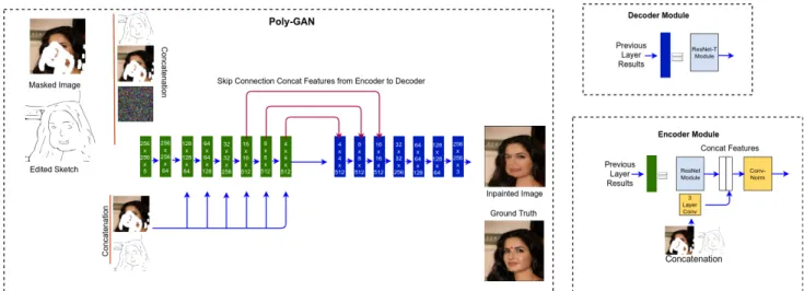
The Poly-GAN architecture, shown in Figure 3.4, follows the encoder-decoder style of generator. The discriminator architecture is shown in Figure 3.5. The network architecture is inspired by recent developments in generative adversarial networks, and includes some unique features. We explain the details of our architecture next.

3.3.2.1 Encoder

The encoder in our architecture, shown in Figure 3.4, can be divided in three main components, a) Conv Module, b) ResNet Module, and c) Conv-Norm Module. We discuss the use of two new modules that are Conv Module and Conv-Norm Module. The ResNet module follows the standard architecture of residual networks [39].

Conv Module. Conditional GANs [7], [31] have conditional inputs at the first layer. e.g., the source image or latent noise. An important benefit of our architecture is that it includes conditional inputs at every layer, instead of only having conditional

(55)

Figure 3.4: Poly-GAN architecture. The left side shows the encoder in green and decoder in blue. The example shown is for garment transformation (Stage 1) but the architecture is the same for image stitching and inpainting. The conditions of reference garment and body pose are fed at all of the encoder layers. Skip connections from coarse layers of the encoder are fed to the corresponding layers of the decoder. The top right block shows the decoder module and the bottom right block shows the encoder module.

Figure 3.5: Architecture of the Discriminator. The example shown is for garment trans-formation but the architecture is the same for image stitching (Stage 2) and inpainting (Stage 3).

(56)

inputs at the first layer. We observed that if the conditional input is limited to the first layer, then its effect diminishes as the features propagate deeper in the network. As a result, there is hardly any conditional information left in deeper layers. We decided to feed the conditional inputs at every layer through a Conv module shown in the encoder module of Figure 3.4. The Conv Module consists of 3 convolution layers, each followed by a ReLU activation function which outputs the number of features required in the layer under consideration.

Conv-Norm Module. The ResNet module outputs newly learned features, which are concatenated with the features learned from the Conv Module. There is significant difference between the features from ResNet and features from the Conv Module. Thus, we pass the concatenated features to the Conv-Norm module to take advantage of the variation in features from the two modules. The Conv-Norm mod-ule has 2 convolution layers, with each convolution layer followed by an instance normalization layer and activation function.

3.3.2.2 Decoder

The decoder part of the network learns to generate the desired image based on the features encoded by the encoder. The decoder part of Poly-GAN, shown in the decoder block of Figure 3.4, is similar to the decoder used in other GANs, e.g., Cycle GAN [40]. The decoder consists of a series of ResNet modules followed by transposed convolution to up-sample the input in each block. However, there are fewer layers in the decoder which receive information from the encoder through skip connections.

3.3.2.3 Skip Connections

One of the important design decisions of Poly-GAN is the placement of skip con-nections. From previous works [21], it is understood that coarser spatial resolution results in higher level spatial change, such as pose and shape. We use skip

(57)

connec-CHAPTER 3. FASHION SYNTHESIS

tions to pass the information from the encoded coarse layers (4x4, 8x8, 16x16) to the respective decoder layers (4x4, 8x8, 16x16) and concatenate to augment the fea-ture representation. We observed that if we use skip connections between encoder and decoder at spatial resolution above (16x16), then the generated image is not de-formable enough to be close to the ground truth. If we don’t use skip connections above spatial resolution of (16x16), then the problem of missing minute details arises in the generated image. This is illustrated in the results of Figure 3.7. Using skip connection to connect all layers of the encoder to their respective decoder layer would help in passing minute details from the encoder side, but would also hinder learning and generating new images effectively.

3.3.3 Discriminator

The discriminator used in our experiments is the same discriminator used in the Super Resolution GAN [14]. The architecture of the discriminator is shown in Figure 3.5. The reason behind the selection of the discriminator is to penalize for blurry images, which are often generated by GANs using the L2 loss function.

3.3.4 Loss Function

Our loss function consists of three components: adversarial loss Ladv, GAN lossLgan

and identity loss Lid. The total loss and its components are presented below, where

D is the discriminator, Gis the generator, xi, i= 1, ..., N represent N input samples

from different distributions pi(xi), i= 1, ...N, t is the target,F are fake labels andR

are real labels.

min

G LGAN =λ3Ex1∼p1(x1),..,xN∼pN(xN) kD(G(x1, .., xN)−Rk2₂

(58)

CHAPTER 3. FASHION SYNTHESIS min D LAdv =λ1Et∼pd(t)kD(t)−Rk 2 2+ λ2Ex1∼p1(x1),..,xN∼pN(xN) kD(G(x1, .., xN)−Fk2₂ (3.2) LId=λ4Et∼pd(t),x1∼p1(x1),..,xN∼pN(xN) kG(x1, .., xN)−tk1 (3.3)

In the above equations,λ1toλ4are hyperparamters that are tuned during training.

We use the L2 function as the adversarial loss for our GAN, similar to [15]. We also

use the L1 function for the identity loss, which helps reduce texture and color shift

between the generated image and the ground truth. We considered adding other loss functions, such as the perceptual loss [16] and SSIM loss [17], but they did not improve our results.

3.4 Experiments

3.4.1 Training Methodology

The work on StyleGAN [21] revealed certain input conditions that contributed to the generation of super realistic images, improving upon the blurry or distorted images generated by previous works. These conditions are a) images in the dataset should be of similar zoom ratio; b) the input to the GAN should be simple; c) diversity of the data should be balanced. In our initial experiments with DCGAN [41], Pro-gressiveGAN [8], CycleGAN [40], and StyleGAN, we observed that if we pass the whole body with the head attached, then the results are blurry and the GAN fails to generate properly. In our experiments we made sure that the dataset is clean enough

(59)

to have similar zoom ratio on the subject, images are diverse, and we removed any complex distractions, such as the head, before passing to the Poly-GAN inputs.

We chose to use the RGB skeleton over a binary image of the pose. Our decision was based on the observation that color coded feature presentation are more effective. The other important observation we made while experimenting with Poly-GAN is that the results are affected by the order in which the conditions are concatenated and we adjusted the inputs accordingly. We used hyperparameters similar to CycleGAN [40] for Poly-GAN training. We used a learning rate of 0.0002, an Adam optimizer with β1 = 0.5 and β1 = 0.999, batch size of 1 in all our experiments, and image

size of 128x128 to feed images in the network. We also used an image buffer during training similar to the one suggested in [42]. The image buffer helps in stabilizing the discriminator by keeping a history of a fixed number of generated images which are randomly passed to the discriminator. All the experiments are performed on a workstation with 16GB of RAM using an Nvidia 1080ti GPU and Ubuntu 16.04.

3.4.2 Dataset

We follow the process used in VITON [22] while creating our training and testing datasets from the publicly available DeepFashion dataset [34]. We use LCR-net++ [35] for 2D human pose estimation, and Pytorch-MULA [37] [38] to get the parsing results for the models. The human parser [37] is used to create data to train U-Net++ [32], to segment the garments from the models, and to remove the head from the models. We have 14,221 training samples, as in the VITON dataset, and 900 paired samples for testing our method. We note that the authors in VITON [22] have used [43] for human parsing and [44] for 2D human pose estimation.

(60)

Table 3.1: Fashion Synthesis Quantitative Results. Bold numbers indicate best perfor-mance. Metric Method SSIM IS CP-VTON 0.6889 2.6049 Poly-GAN Stage 2 0.7174 2.8193 Poly-GAN Stage 3 0.7369 2.6549 Poly-GAN Stage 4 0.7251 2.7904 3.4.3 Quantitative Evaluation

We use the Structural Similarity Index metric (SSIM) [17] and Inception Score metric (IS) [45] which are widely accepted metrics for evaluation of images generated by GANs. SSIM predicts the similarity between two images, where the higher the score the better the network is in generating realistic images. The Inception Score compares the quality of an image to human level grading, and is sensitive to blurring in an image. We compare our results to the state of art method CP-VTON [23]. Since the code for CP-VTON is publicly released [46], we are able to obtain results on our dataset for comparison. The state of the art method MG-VTON [24] tries to solve the problem in a significantly different way than ours, but unfortunately their code is not available. Therefore, our comparison was limited to CP-VTON. We perform our evaluation on test data that consist of 900 paired images. The results are shown in Table 3.1. SSIM and IS scores are included for the final stage of Poly-GAN, as well as for Stages 2 and 3 (after stitching the head of the model). The results illustrate that Poly-GAN outperforms CP-VTON in all cases. By comparing the scores of different stages, we see that the output of Stage 2 is the sharpest and has the highest IS score, but it suffers from holes due to blank regions. The output of Stage 3 has the highest SSIM score, i.e. is the most similar to the desired output, but it suffers from blurriness artifacts. The combination on the two gives a balanced score without

(61)

Figure 3.6: Poly-GAN results shown from left to right column: Model image; Pose Skele-ton; Reference Garment; Stage 1: transformed garment; Stage 2: garment stitched on segmented model; Stage 3: refinement of outputs from stage 2: Stage 4: post-process result from stage 2 and stage 3 with head in original model image.

scoring the highest for either metric.

3.4.4 Qualitative Evaluation

We provide a visual comparison of our results with CP-VTON in Figure 3.8. Our Poly-GAN method is able to keep body parts intact. especially in cases where the arms occlude the body. For example, in Figure 3.8 the second image from top shows that CP-VTON fails in the case of self occlusion which our method is able to handle in almost all cases. Poly-GAN is able to precicely map the generated garment from Stage 1 (see Figure 3.3) to the missing garment region on the body in Stage 2, thus avoiding the spill of color, which is evident in CP-VTON.

(62)

Figure 3.7: Poly-GAN results shown from left to right column: Model image; Pose Skele-ton; Reference Garment; Stage 1: transformed garment; Stage 2: garment stitched on segmented model; Stage 3: refinement of outputs from stage 2: Stage 4: post-process result from stage 2 and stage 3 with head in original model image.

(63)

Figure 3.8: Comparison examples of Poly-GAN with CP-VTON. Shown in columns from left to right: model image, reference garment, CP-VTON result, Poly-GAN result.

(64)

suffer from slight color shift in some samples, which is a common problem with GANs that are asked to generate colors from various distributions. One limitation of our method is texture preservation when generating letters, graphics or patterns that are present in the reference garment. This artifact is due to the use of a GAN to reshape the garment, instead of using image warping methods. A less pronounced artifact in some images is a visible boundary outline that is caused by errors in the segmentation by U-Net++. This limitation can be overcome by using a larger and more diverse dataset for training.

For qualitative evaluation, we also present images that were randomly generated with StyleGAN in Figure 3.9. It is evident that although StyleGAN is not conditioned on pose, the generated images suffer from color spill due to occlusion and artifacts in preserving textures and graphics on the garments.

3.5 Conclusion

We offer a novel approach to the Fashion Synthesis problem by introducing Poly-GAN, a new multi-conditioned GAN architecture that is suitable for many tasks. Qualitative and quantitative results on DeepFashion demonstrate the benefits of our approach by achieving state of the art results. Future research will focus on further exploring the Poly-GAN architecture for a variety of applications.

(65)

Chapter 4

Discussion

In current state o the art methods, selecting a right Generative Adversarial Archi-tecture is typically task dependent, where some archiArchi-tectures perform a task better than others. In our work, we try to find a common type of architecture that can be applied across several tasks with minimal modifications. We focus our work notably in conditional Generative Adversarial Network, which are known to be able to manip-ulate generated images based on certain input criteria. We present a new architecture named Poly-GAN and demonstrate that it is suitable for many tasks.

An interesting characteristic of Poly-GAN is that passing the conditional input in every layer helps the GAN converge faster with less data and less training resources compared to many existing architectures. Traditional conditional GANs have input only in the initial layer, and consequently performance suffers from information loss as the features propagate deeper in to the network. The progressive GAN architecture demonstrated that when the GAN setup is generating coarse images at low resolution, then it is easier to stabilize the setup. As is the case of Progressive GAN, we observe that it is easier to manipulate coarse level information with a conditional input passed to each layer and shared with the decoder using skip connections.

We test our network in multiple applications, specifically fashion synthesis and image inpainting. We observer that our model not only converges with less data, but also performs equally well or better than state-of-the-art methods.

(66)

CHAPTER 4. DISCUSSION

Based on our work we can conclude the following points:

• For a network to learn efficient attributes of an image, we need to pass

dis-tinct conditions as hints to the network. Disdis-tinct hints/conditions can help the network learn important or required image characteristics with less training data.

• Manipulating the features of each layer through a conditional input is much

easier than doing the same with traditional encoder and decoder networks.

• Multiple tasks can utilize a single network architecture if proper conditions are

provided to the network according to the task.

• Few loss functions, such as L2 or L1 and GAN loss, are sufficient for a cGAN

network to converge. We find that perceptual loss is useful which helps in retaining color in the generated images.

• We emphasize the skip connections between coarse layers from the encoder to the decoder, because these connections enforce spatial information, which is especially useful in tasks like fashion synthesis.

• We can increase the resolution of a generated image by increasing the layers in