http://www.imdea.org/socialsciences http://repec.imdea.org [email protected]
in Economics and Social Sciences
Ctra. Colmenar Viejo km. 14, 28049 Madrid, Spain
ciencias sociales
working
papers series
www.imdea.org
2010/17
House prices and risk sharing
Dmytro Hryshko,
María José Luengo-Prado and Bent E. Sørensen
Dmytro Hryshko
University of Alberta
Mar´ıa Jos´e Luengo-Prado
Northeastern University Bent E. Sørensen University of Houston and CEPR July 30, 2010 Abstract
Homeowners in the Panel Study of Income Dynamics are able to maintain a high level of consumption following job loss (or disability) in periods of rising local house prices while the consumption drop for homeowners who lose their job in times of lower house prices is substantial. These results are consistent with homeowners being able to access wealth gains when housing appreciates as witnessed by their ability to smooth consumption more than renters. A calibrated model of endogenous homeownership and consumption is able to reproduce the patterns in the data quite well and provides an interpretation of the empirical results.
working
1. Introduction
Many countries, including the United States, experienced large fluctuations in house prices over the last decade. For example, house prices increased by 75 percent from 2001 to 2005 in the Providence, R.I., Metropolitan Statistical Area (MSA), while Los Angeles, on the opposite coast, saw a gain of 91 percent.1 However, Providence house prices declined
by 18 percent from 2006 to 2010, while those of Los Angeles fell even more, by 22 percent. As housing is the largest asset for most families, such price movements are associated with large swings in consumers’ net worth and it is of first-order importance to understand the impact of these fluctuations on consumption.
Homeowners are able to maintain their level of nondurable consumption after income losses when house prices are increasing but during deep recessions, such as the subprime crisis that started in 2007, the drop in consumption can be severe for homeowners who become displaced or disabled. Our point estimates imply that job displacement for a homeowner in the Providence MSA would result in a drop in nondurable consumption during 2006–2010 that is more than 28 percentage points larger over this four-year period than it would have been during 2001–2005.2 The effect of house prices would be even
larger in cities such as Los Angeles and housing depreciation is likely to provide a severe drag on the recovery of the aggregate U.S. economy from the subprime crisis.
The individual-level data are from the Panel Study of Income Dynamics (PSID) and the focus is to study consumption changes following the onset of disability or job displace-ment (arguably exogenous shocks to income). In particular, we investigate households’ ability to maintain—“smooth”—consumption in the face of such shocks and the empiri-cal focus is on deviations from countrywide fluctuations, or “risk sharing.” Risk sharing 1First quarter data from the Federal Housing Finance Agency (FHFA), formerly known as the Office
of Federal Housing Enterprise Oversight.
2These numbers are calculated using Table 1, column (2).
working
is interesting per se and focusing on risk sharing allows us to abstract from a host of difficult-to-control-for aggregate variables that may affect consumption. The main con-tribution is to study how risk sharing varies with house-price appreciation by matching PSID data and house price data at the metropolitan level from the FHFA—house-price appreciation arguably provides exogenous shocks to homeowners’ wealth and collateral.3
The core empirical result is that homeowners maintain relatively higher (lower) levels of nondurable consumption after job displacement or disability when house values increase (decrease).
To interpret the findings, we calibrate and simulate a life-cycle model of households with preferences for housing (shelter) and nondurable consumption. The model captures the main features of homeownership—in particular the role of housing as both a con-sumption good and an asset: homeownership is endogenous and housing services can be obtained either in the rental market or through homeownership. Households adjust (nondurable, non-housing) consumption, and possibly housing, in response to income fluc-tuations although buying or selling a house requires paying a proportional commission which makes the effect of house price shocks more complicated than the effect of liquid wealth shocks, such as winning the lottery. For homeowners with housing equity above a minimum down payment a positive capital gain in housing is fully liquid—although the household may choose to upgrade to a larger house while paying a proportional com-mission. Homeowners who own less than the minimum down payment will only be able to access capital gains in housing if housing appreciation pushes their equity above the required minimum. In the face of a persistent negative shock to housing, a homeowner may choose to downsize or move to rental housing—in particular, if the shock happens at 3The PSID has information on household home equity, but these data are questionable for the present
purpose, because household-level equity is likely endogenous. Some regressions using self-reported home equity are tabulated in a appendix.
working
the same time as a persistent income loss.
Panel-data regressions are performed on simulated data in the same fashion as in the real data and the estimated parameters from the data and from model simulations are compared, and—to the degree that magnitudes match between actual and simulated data—interpreted. The simulations show that homeowners maintain consumption better than renters when the relative price of housing increases.
The model leaves out many real-world complications; nonetheless, the predictions of the model match the results from the PSID well. We do not attempt to structurally fit the model as Li, Liu and Yao (2009) who have a different focus but use a similar model. The disadvantage of the present approach, compared with a structural approach, is that one cannot test the model while the advantage is that the empirical findings are robust to many forms of model misspecification.
Related work has attempted to measure the direct impact of housing appreciation on consumption—typically under the label of “wealth effects.” Because national house prices correlate with economic conditions in general, the quantification of the effect of house prices on consumption remains controversial. The most promising avenue seems to be regressions that rely on regional house prices as pioneered by Attanasio and Weber (1994)—such regressions allow for control of nationwide effects. Further, these authors simulate a theoretical model to evaluate the plausibility of their empirical estimates. Two papers in that vein are Campbell and Cocco (2007), who find evidence of a wealth effect, and Attanasio, Blow, Hamilton and Leicester (2009), who argue that common causality is a more likely explanation for the patterns of consumption and house-price growth in the United Kingdom. Like these authors, this article uses regional house prices and compares renters to owners, and young households to old households.
Several other papers are related to the present article: Hurst and Stafford (2004)
working
document that house equity is used as a mechanism to smooth income shocks due to un-employment. Their empirical focus is on the decision to refinance while this work directly considers consumption. Lustig and Van Nieuwerburgh (2010) find more risk sharing be-tween U.S. metropolitan areas in periods when average U.S. house-price appreciation is high.4 Chetty and Szeidl (2007) study consumption patterns when a part of wealth is
“committed” and cannot be easily adjusted as is the case for our consumers in the sense that it is costly to adjust housing consumption. Finally, Leth-Petersen (2010) considers the effect of increasing the ability to use housing as collateral by studying the effect of an exogenous relaxation of home-equity lending restrictions in Denmark.
The empirical strategy is described in Section 2 while the data and empirical es-timations are presented in Section 3. The theoretical model and its implications are in Section 4 while Section 5 reports the results of regressions using simulated data. Section 6 concludes.
2. Regression specification
In an endowment economy with one nondurable good, complete Arrow-Debreu markets and constant relative risk aversion utility, all consumers will have identical consumption growth rates. Mace (1991) tests this prediction in a panel-data regression of consumption on income with controls for aggregate effects while Cochrane (1991) examines whether consumers are fully hedged against job loss. Let zit = logZit−logZit−4 be the growth
rate of a generic variable Z, such as consumption C, of individual i from year t−4 to
t, and let ¯zt be the period t specific mean of any generic variable z. Let hpmt be the
four-year growth rate of house prices in the metropolitan area m where individual i lives 4Lustig and Van Nieuwerburgh (2010) consider the role of housing collateral in a general equilibrium
model with state-contingent claims. However, they use U.S.-regional data and do not consider renters versus homeowners.
working
and letDit be a dummy taking the value 1 if the head of householdi suffers displacement
and 0 otherwise. Alternatively, Dit is an indicator that takes the value 1 at the onset
of disability, –1 if the household head exits from disability, and 0 otherwise. Pooling data from regions with different house-price appreciation, we examine the impact of job loss (disability) on consumption and the risk-sharing role of housing in the face of job displacement (disability) by estimating the relation
cit−c¯t=µ+β (hpmt−hpt) +ξ (Dit−D¯t) +ζ (Dit−D¯t)×(hpmt−hpt) + (Xit−X¯t)0δ+εit, (1)
where Xit is a vector of controls (age, the square of age, and family size). The
time-specific mean is subtracted from all variables because the subtraction of the aggregate non-diversifiable component gives all estimated coefficients the interpretation of showing deviations from perfect risk sharing. In particular, by subtracting hpt fromhpmt, the
na-tionwide average house-price appreciation is removed from the time-varying coefficient— the time-series variation in average house prices is likely correlated with other aggregate variables, such as stock market performance, and we want to hedge against house prices capturing such variables. Here, the derivative of idiosyncratic consumption growth with respect to a disability (displacement) shock is ξ+ζ(hpmt−hpt), which would be 0 under
perfect risk sharing. When these coefficients are not 0, a positive coefficient of ζ im-plies that house-price appreciation dampens the effect of displacement on consumption growth—that is, risk sharing goes up with house-price appreciation. The regressions are similar to those of Cochrane (1991) with a house-price interaction added.5 Briefly, under
full insurance of nondurable consumption and housing services, deviations of idiosyncratic 5Cochrane (1991) estimates cross-sectional regressions but panel data regressions with time fixed
effects can be seen as weighted averages of cross-sections. Cochrane’s definition of involuntary job-loss is essentially the same as the present definition of “displaced” and the regressions confirm his results. (Cochrane (1991) also leaves out income).
working
consumption growth from the nationwide average should be orthogonal to the deviation of an idiosyncratic shock-to-income (such as disability or displacement) from the nation-wide average, as well as its interaction with regional house-price growth, assuming house prices are uncorrelated with measurement error in consumption and shocks to the relative taste for consumption of nondurables and housing services. That is, under the null of full insurance, the coefficients β, ξ, and ζ should be equal to zero. If, however, the risks to nondurable consumption are shared nationally but the risks to consumption of housing services are shared within a region, only ˆξ and ˆζ should be statistically indistinguishable from zero.6 See Appendix A for derivation of equation (1).
3. Empirical estimations
Individual- and household-level data are from the PSID, which is a longitudinal study of U.S. households. We briefly describe the estimation sample; for more details on sample selection, see Appendix B.
The PSID maintains Geocode Match Files, which contain the identifiers necessary to link the main PSID data to Census data which allows for adding data on characteristics of each respondent’s neighborhood to the already rich array of socioeconomic variables collected in the PSID.7 Households are matched to their MSA of residence and house-price
appreciation is at the metropolitan level.
Food consumption is used as the measure of consumption because of a lack of broader consumption aggregate, although results are also shown for imputed nondurable con-6More briefly, income growth is included in the regressions. Income growth is more likely to be
endogenous to shocks to desired consumption or correlated with left-out regressors and results without income included are presented first. However, the results are robust to the inclusion of income because income is obviously correlated with displacement and job loss.
7The Geocode Match data are highly sensitive (usually pinpointing the census tract in which families
live), and are available only under special contractual conditions designed to protect the anonymity of respondents.
working
sumption. Food consumption consists of food consumed at home and away from home (excluding food purchased at work or school). Household income is the sum of real labor and transfer income of head and wife before taxes. Food consumption at home and away from home and household income are deflated by the all-items-less-housing consumer price index (CPI) from the Bureau of Labor Statistics.
A household head is considered displaced if the head’s “previous company folded or changed hands or moved out of town; employer died, went out of business,” because of “strike, lockout,” or because the head was “laid off/fired.”8 The disability variable is
constructed from two questions typically referred to as “limiting conditions.”9 The first
asks: Do “you (head) have any physical or nervous condition that limits the type of work or amount of work you can do?” The second question asks: “How much does it limit your work?” We assume the head is disabled if he or she answers yes to the first question and states “can do nothing ” or indicates disability limits the ability to work somewhat or a lot.
Because food consumption is imprecisely measured at the annual frequency, four-year (overlapping) growth rates are used. This choice reduces measurement error and averages out temporary fluctuations in income and consumption. Economists typically agree that longer-lasting (“permanent”) shocks matter more for welfare, so little is lost by looking at the longer frequencies where permanent shocks are relatively more important.10
In the regressions, the disability variable enters as 0 if there was no change in the disability status from period t−4 to t, as 1 if the head reports disability at t but not at
t−4, and as –1 if the head reports disability at t−4 but not at t. The displacement variable enters as 1 if the head reports being displaced in year t−3, t−2, t−1, or t.
8The PSID did not collect information on displacement during the 1994–1997 waves.
9In 1973, 1974, and 1975, only new heads were asked these questions. In cases where the answer in
one of those years is missing, we impute it using the answer from a preceding year.
10Cochrane (1991) uses three-year growth rates, similar to our frequency. An even number of years is
used here to match up with the biennial sampling frequency initiated by the PSID in 1997.
working
When presenting results by housing tenure status, a homeowner (renter) is a household that owned a house (rented) in all periods involved in calculating the consumption growth rate.
The analysis is restricted to families with stable composition (same head and wife during the four-year span), whose head of household is of prime age (25–65) with infor-mation on housing status and region of residence during the four-year span. The Latino and Immigrant samples of the PSID are excluded but households from the representative core sample and the Survey of Economic Opportunities (SEO), the sub-sample of low income households, are included. The sample is also restricted to households that reside in the same metropolitan area during a given four-year period so they can meaningfully be assigned four-year MSA house-price changes—households that move within the MSA remain in the sample.
Total (imputed) nondurable consumption. Consumer research typically focuses on the response of total nondurable consumption and Blundell, Pistaferri and Preston (2008) impute nondurable consumption of PSID households in a study of consumption and in-come inequality. Using data from the Bureau of Labor Statistics’ Consumer Expenditure Survey (CEX) for 1980–1992, these authors estimate a structural equation for food con-sumption as a function of nondurable concon-sumption and demographics and invert the estimated equation to obtain a measure of nondurable consumption for PSID households. We follow their imputation strategy using extracts of the CEX for 1980–2002 from the NBER.
In the CEX, households report at most four quarterly observations on consumption components and only households that respond in all four quarters are included. If con-sumption is recorded in yearstandt+1, annual consumption is assumed to refer to yeart
if that year contains at least six months of records and to yeart+ 1 otherwise.11 The final
11In the PSID, males are considered household heads, while in the CEX the head is the person who
working
CEX sample consists of households with heads 25–65 years old and born between 1915 and 1978. Nondurable consumption is the sum of annual expenditures on food, alcohol and tobacco, clothes and personal care, domestic services, transportation, entertainment, gambling and charity, and utilities.
Table A-3 reports the results of an IV-regression of food consumption on nondurable consumption, demographic controls, and prices.12 The estimated coefficients in Table A-3
are used to impute nondurable (non-housing) consumption to PSID households for 1980– 2002.
House-price appreciation. MSA house-prices are from the FHFA, which reports quar-terly house-price indices for single-family detached properties.13 Merging FHFA houses
with PSID data results in a sample that covers 1976–2005. The overall mean (four-year) house-price appreciation is 6 percent, with a 19 percent standard deviation while median house-price appreciation is lower at 4 percent. There is rich variation across MSAs and over time during this period. Three of the MSAs with lowest house-price appreciation dur-ing the period are Bdur-inghamton, Houston, and New Orleans, which have a mean (standard deviation) appreciation of –7.7 (13.5), –5.7 (14.5), and –3.3 (13.4) percent, respectively. Three of the MSAs with the highest house-price appreciation are the Boston, San
Fran-rents or owns the residential unit. To make the definitions of heads compatible, we assign the male to be the head for CEX couples. Households whose heads are part-time or full-time college students are dropped. As for the PSID sample, observations with zero or missing records for food consumption at home are dropped and the annual distribution of total food is trimmed at the 1st and the 99th percentiles.
12In an OLS setting, the estimated elasticities may be biased because of measurement error in
non-durable consumption and because of endogeneity of food and nonnon-durable consumption. The regressions follow Blundell et al. (2008) and instrument log-nondurable consumption (and its interactions with year and education dummies) with the head’s sex-education-year-cohort specific averages of log hourly wages (and their interactions with year and education dummies).
13The agency bases these reports on data on conventional conforming mortgage transactions obtained
from the Federal Home Loan Mortgage Corporation (Freddie Mac) and the Federal National Mortgage Association (Fannie Mae). The house-price indices are based on the methodology proposed by Case and Shiller (1989) and they are deflated by the all-items-less-housing CPI. The index for each geographic area is estimated using repeated observations of housing values for individual single-family residential properties on which at least two mortgages were purchased or securitized by either Freddie Mac or Fannie Mae since January 1975.
working
cisco, and New York City areas, at 15.3 (28.2), 14.7 (22.9), and 11.5 (24.5), respectively. See Appendix C for more details.
3.1. Estimation results
The regressions described in Section 2 are estimated using a two-stage Prais-Winsten GLS procedure, which is efficient in the case of first-order autocorrelation; the observations are overlapping and therefore, by construction, autocorrelated.14 The standard errors are
calculated using robust clustering at the MSA level.
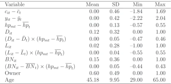
The range of four-year log differences of consumption is between –1.8 and 1.7, while that of income is even larger. House prices also show large deviations from the U.S. mean. On average, about 12 percent of the sample receives a displacement shock during a four-year time span, while 5 percent suffers from a limiting condition and 3 percent recovers from one—see (appendix) Table A-1.
Table 1 shows results for owners, renters, and the pooled sample. Disability and displacement are first considered separately and then combined into a variable called “bad news.” Bad news is a dummy variable that equals one if a household head becomes either displaced or disabled (or both). The results for homeowners in columns (1) and (2) indicate that the main effect of disability or displacement is similar with a drop in nondurable consumption of about 4 percent. The direct impact of house-price appreciation is robustly estimated at about 14 percent for owners. The interaction of house prices with disability is very large, estimated at about 0.33, while the interaction with displacement is about 0.16. In the regression using bad news—column (3)—the main effect of bad news is –0.05 while the interaction term is 0.18. These numbers imply that nondurable consumption drops by about 5 percent when the household head becomes disabled or 14The data will have autocorrelation of order higher than one but typically most efficiency gains are
obtained as long as first-order correlation is allowed for.
working
displaced in the absence of house-price appreciation but if house prices appreciate by 10 percent over the relevant four-year span, the drop in nondurable consumption is only about 3 percent (ignoring the main effect of house-price appreciation).
For renters, there is a large direct effect of house prices which likely is due to house prices being correlated with components of income or with expectations of future income. The interaction of disability and displacement with house-price growth is negative for renters with a larger (although insignificant) coefficient for disability. The direct effect of disability is estimated at –0.06, and the direct effect of displacement at –0.08. Combining these into bad news we find a coefficient of –0.07 while the interaction term becomes very close to 0—the variable “bad news” delivers less noisy results and, in the following, we use this variable only. The last column shows the results for a combined sample of owners and renters and the results are in-between those found for each of these samples.
Table 2 explores different samples and specifications in order to explore robustness and add to our understanding. Only the direct effects of house price growth, bad news, and their interaction are presented to conserve space. The table includes a column for owners and one for renters and, for convenience, repeats the results of Table 1 as the first entry. The second entry limits the sample to households that did not move during each four-year period. This addresses the issue of whether households free up home equity by downsizing their residence after being hit by a bad news shock. However, the results are similar to the baseline case and the insurance effect of house-price appreciation is therefore not mainly a result of downsizing. The results are also robust to using non-overlapping intervals although the interaction terms are large for both owners and renters, yet not significant for renters. The non-overlapping regressions are clearly estimated with less precision.
The large coefficient to house-price appreciation for renters is puzzling. Household
working
income may contain a regional component correlating with house-price growth and an attempt was made to extract the component of house-price appreciation orthogonal to income by regressing house-price appreciation on average income growth in the MSA and using the residuals as our measure of house-price appreciation.15 This lowers the
estimated coefficient to house-price appreciation slightly for renters but does not change the coefficients to any variable strongly. These results highlight how careful one needs to be in interpreting aggregate correlations between appreciation of house values and nondurable consumption as causal. The next two sets of results consider young and old households, respectively. Consumption of young renters reacts positively to house-price appreciation consistent with a correlation of house-house-price appreciation with income expectations; however, the interaction term is insignificant for young owners as well as renters. Older individuals are hit harder by bad news. Old owners and, in particular, old renters react less strongly to house-price appreciation while the interaction term is highly significant for older owners only. The latter result may reflect that older homeowners, on average, have a larger amount of accumulated housing equity that helps them insure nondurable consumption.
Table 3 presents further robustness results. The interaction effect may be due to changes in house prices tightening or loosening credit constraints. Poorer households may be subject to tighter credit constraints and households in the SEO sample, the subsample of low-income households, may have larger interaction terms than individuals in the representative core sample. The interaction term is slightly larger for the SEO sample but the difference is not statistically significant.16
15MSA income is per capita real income received by all persons from all sources and is available from
the Bureau of Economic Analysis.
16We explored a little further and found that the interaction term is higher for SEO households with low
home equity relative to consumption which is consistent with this group having to adjust consumption more in the case of bad news and negative shocks to house prices. We explore the role of home equity in more detail following the presentation of the model.
working
Table 3 further shows two sets of results for the sample split into an early period 1980– 1994 and a late period 1994–2005.17 This split results in a similar number of observations
for different subsamples. If financial liberalization and higher use of home-equity lines of credit made housing equity easier to access one would expect to find more consumption insurance in the latter sample. However, the results are very robust to the sample period. Likely, people with liquid life-cycle savings were able to draw on those in the early sample, possibly by taking out a second mortgage.
When imputed nondurable consumption is used, the results for owners are virtually identical to the results using food consumption. For renters, the estimated impact of house-price appreciation is even larger using this consumption measure and the interaction term is larger at 0.098, but this coefficient is still nowhere near significance statistically. While imputed nondurable consumption is surely imperfect, these results do not point to our findings being spurious due to the food-only consumption measure.
Finally, the bottom panel of Table 3 displays results where income is included as a regressor. As expected, the coefficient to bad news becomes slightly smaller because part of the impact is captured by income, but the reduction is not large—likely because income shocks are partly transitory and partly persistent while the bad news shocks are overwhelmingly persistent and not well captured by measured income.
4. The model and calibration
To interpret the results, we introduce a model and perform regressions using simulated data of the same form as those using PSID data. An important feature of the model is 17The disability indicator is used instead of bad news because information on disability was collected
consistently throughout the sample period while information on displacement, used for constructing the bad news indicator, was not collected during 1994–1997. Using bad news instead delivers qualitatively similar estimates: for the 1980–1994 sample the interaction term is estimated at about 0.19, significant at the 5% level, while the interaction term for the 1994–2005 sample is about 0.20, nearly significant at the 10% level.
working
that homeownership is a choice for households (i.e., an endogenous tenure choice). As in D´ıaz and Luengo-Prado (2008) households have finite life-spans and derive utility from consumption of a nondurable good and housing services that can be obtained in a rental market or through homeownership. House buyers pay a down payment, buyers and sellers pay transactions costs, and housing equity above a required down payment can be used as collateral for loans. There are no other forms of credit. Tax treatment of owner-occupied housing is preferential as in the United States. Households face uninsurable earnings risk and uncertainty arising from house-price variation.
4.1. The model
Preferences, endowments, and demography. Households live for up to T periods and face an exogenous probability of dying each period. During the first R periods of life they receive stochastic labor earnings and from period R on, they receive a pension. When a household dies, it is replaced by a newborn and its wealth is passed on as an accidental bequest. Houses are liquidated at death; thus, newborns receive only liquid assets.
Households derive utility from nondurable goods and from housing services obtained from either renting or owning a home. One unit of housing stock provides one unit of housing services. The per-period utility of an individual of age t born in period 0 is
U(Ct, Jt) where C stands for nondurable consumption and J denotes housing services.
Households cannot rent and own a home at the same time. The expected lifetime utility of a household born in period 0 is E0
PT
t=0 (1+ρ)1 t ζtU(Ct, Jt), where ρ ≥ 0 is the time
discount rate and ζt is the probability of being alive at age t.
Market arrangements. A household starts period t with a stock of residential assets,
Ht−1 ≥0, deposits,At−1 ≥0, and collateral debt (mortgage debt and home-equity loans),
Mt−1 ≥ 0. Deposits earn a return ra and the interest on debt is rm. A house bought in
working
periodt renders services at the beginning of the period. The price of one unit of housing stock (in terms of nondurable consumption) is qt, while the rental price of one unit of
housing stock is rft.
When buying a house households must make a down payment, θqtHt.18 Therefore, a
new mortgage must satisfy the condition Mt≤(1−θ)qtHt.For homeowners who do not
move in a given period, houses serve as collateral for loans (home-equity loans) with a maximum loan-to-value ratio (LTV) of (1−θ).
If house prices go down, a homeowner can simply service debt if he or she is not moving; i.e, as long as the homeowner stays in the same house,Mtcould be higher than (1−θ)qtHt
if Mt < Mt−1. Foreclosure is not allowed so a homeowner can be “upside-down” (have
negative housing equity) for as many periods as the household desires.19
Households pay a fraction κ of the house value when buying a house (e.g., sales tax or search costs). When selling a house, a homeowner loses a fraction χof the house value (brokerage fees). Houses depreciate at the rate δh and households can choose the degree
of maintenance. Buying and selling costs are paid if|Ht/Ht−1−1|>0.05 which indicates
that only homeowners upsizing or downsizing housing services by more than 5 percent pay adjustment costs.20
Households sell their houses for various reasons. First, households may want to increase or downsize housing consumption throughout the life cycle. Second, selling the house is 18We abstract from income requirements for people purchasing houses. Many lenders follow the rule of
thumb of “three times income” in determining the size of mortgages. However, the empirical literature finds that wealth constraints are more important than income constraints when people purchase a home. See, for example, Linneman, Megbolugbe, Watcher and Cho (1997) or Quercia, McCarthy and Watcher (2000).
19These assumptions simplify the computation of the model while allowing us to consider both
down-payment requirements and home-equity loans without modeling specific mortgage contracts or mortgage choice. See Li and Yao (2007) for an alternative model with refinancing costs, and Campbell and Cocco (2003) for a discussion of optimal mortgage choice.
20Results are robust to alternative formulations of the adjustment costs such as pure maintenance
or pure depreciation. Our specification, which is in-between the two, is slightly easier to implement computationally with a discrete grid.
working
the only way to realize capital gains beyond the maximum LTV for home-equity loans so households may sell the house to prop up nondurable consumption after depleting their deposits and maxing out home-equity loans. Third, households may also be forced to sell their houses as they are subject to an idiosyncratic moving shock, zt. This shock is
meant to capture the effect of “geographical” mobility stemming from job change and demographic shocks not modeled for simplicity.
The government. The government taxes income,Y, at the rateτy. Imputed housing rents
for homeowners are tax-free and interest payments are tax deductible with a deduction percentage τm so taxable income in period t is Ytτ = Yt −τmrmMt−1. Proceeds from
taxation finance government expenditures that do not affect individuals at the margin. Earnings and house-price uncertainty. Households are subject to household-specific risk in labor earnings and house-price risk common to residents of the same region. For working-age households, labor earnings, Wt, are the product of permanent income and transitory
shocks (Pt, νt and φt, respectively): Wt =Ptνtφt. νt is an idiosyncratic transitory shock
with logνt ∼ N(−σν2/2, σν2), while φt is a transitory displacement/disability (“bad”)
shock which reduces income by a proportion µ with a small probability pφ. In turn,
permanent income is Pt = Pt−1γt²tςt. Thus, permanent income growth, ∆ logPt, is the
sum of a non-stochastic life-cycle component, logγt, an idiosyncratic permanent shock,
log²t ∼ N(−σ²2/2, σ²2), and an additional permanent “bad” shock logςt, which reduces
permanent income by the proportion λt with a small probability pς. λt is allowed to vary
with age, the cut being more drastic for older households.21 Retirees receive a pension
proportional to permanent earnings in the last period of their working life. That is, for a 21The combination of permanent and transitory bad shocks is meant to capture employment and/or
disability shocks that may or may not affect income for more than one period and may affect households differently. We do not have disability and displacement separately in our regressions with simulated data, like in the regressions with PSID data, as we combine transitory and permanent displacement/disability shocks into one indicator for bad news.
working
household born at time 0,Wt=bPR, ∀t > R.22
House prices are uncertain and, following Li and Yao (2007), we assume that house-price appreciation is an i.i.d. normal process: qt/qt−1 − 1 = %t, with %t ∼ N(µ%, σ%2).
This specification implies that house-price shocks are permanent.23 In our benchmark
calibration, these shocks are serially uncorrelated and not correlated with household labor earnings.
4.2. Calibration
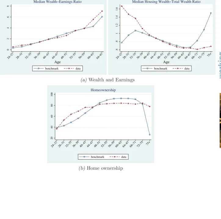
The calibration is constructed to reproduce three statistics from the Survey of Con-sumer Finances: the homeownership rate, the median wealth-to-earnings ratio for working-age households, and the median ratio of home value to total wealth for homeowners (70 percent, 1.8, and .82, respectively).
To match the targets, the discount rate is set to 3.45 percent, the weight of housing in a Cobb-Douglas utility function to .2, and the minimum house-size that consumers can purchase is 1.65 times permanent income. The general strategy in choosing the remaining parameters is to focus whenever possible on the empirical evidence for the median household (see Appendix D for details and Table 4 for parameter values).
5. Regression results from simulated data
Simulations are performed for 27 “regions” with 5,000 people each for a number of periods. House-price shocks are common to all individuals in a given region (there are only three possible house-price shocks), while all other shocks (income and moving shocks) 22This simplification is required for computational reasons and is common in the literature. See, for
example, Cocco, Gomes and Maenhout (2005).
23This assumption is common in the literature (e.g., Cocco 2005, Campbell and Cocco 2003), and greatly
simplifies the computation of the model by facilitating a renormalization of the household problem with fewer state variables.
working
are idiosyncratic. In regions 1 through 9, the house-price shock is at the lowest value for the last four periods (house-price depreciation). In regions 10 through 18, the house-price shock is at the middle value (constant house prices), while in regions 19 through 27, the house-price shock is at the highest value (house-price appreciation). Simulated data from the last five periods (which represent 10 years, as one period in our model corresponds to two years) is used in these regressions.24
To match the specification in the empirical section, four-year log differences in con-sumption, income, and house prices, and overlapping growth rates are used in the regres-sions. The bad news dummy equals 1 in period t if the household suffers a bad shock in periods t, t−1, t−2 or t−3 and not in t−4. As in the data, when presenting results by tenure status, a homeowner (renter) is a household that owned (rented) a house in all periods involved in calculating the consumption growth rate. To facilitate comparisons with the empirical results, regressions are estimated using households with heads aged 28–64. (As explained in Appendix D, households are born at age 24 and retire at age 66.) Table 5, first panel, shows that 10 percent house-price appreciation results in a 2.7 percent increase in nondurable consumption for owners with no effect for renters. The direct effect of bad news is a drop in nondurable consumption of 17 percent for owners versus 21 percent for renters. The coefficients are estimated very precisely—the t-statistics are much larger than those in the data which reflects that the model is a simplification where all consumers are a priori identical. Importantly, the sensitivity of consumption to income changes goes down when houses appreciate as shown by the estimated positive coefficient for the interaction term. Nondurable consumption drops by about a percent less if housing appreciates by 10 percent. Compared to the data, the coefficient to house prices is larger, maybe reflecting higher costs or more stringent financing constraints for
24Results are similar if more periods are included in the regressions.
working
some households in the real world. The effect of bad news is smaller in the real world while the interaction is smaller in the model—maybe reflecting informal help from family (who may live in the same MSA) or assets not present in the model.
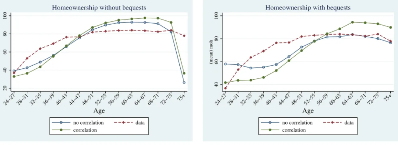
The other panels in Table 5 explore the properties of the theoretical model in order to understand the impact of relative house prices, financing constraints, etc. on our results. The second panel shows the results for the case where there is no homeownership and “house prices” simply capture changes in rental prices. In this case, house-price changes do not affect nondurable consumption directly or through the interaction with the bad-news shock. This set of results verifies that the findings regarding house prices are not due to changes in relative prices per se which, of course, reflects the specific utility function we use.25
The next set of results analyzes a model where homeownership can be obtained with no down payment. In this case, the barriers to home ownership are a minimum required size of the house and the potential trading costs if the house has to be sold again. These results are quite similar to the benchmark case, although the interaction effect is slightly larger because a larger fraction of home equity can be used as collateral for loans. If, alternatively, there is a down payment but no transaction costs, the interaction term gets somewhat smaller as homeowners can easily downsize making home equity completely liquid—talking about collateral in this case is purely semantics. The direct effect of bad news for renters is larger because they are less affluent in this simulation. Interestingly, there is a significant effect of house prices for renters. This effect can, for example, be due to older renters giving up on accumulating enough savings for a down payment and using part of their accumulated savings for nondurable consumption. The negative significant 25The within-period preferences over consumption of nondurables and housing services are of
Cobb-Douglas type. Thus, in the perfect rental market setting, consumers keep fixed proportions of their spending on each type of good: if house prices go up, consumption of housing services goes down but nondurable consumption remains unchanged.
working
interaction could be due to young renters saving for a down payment.
If there is no down payment, adjustment costs, or minimum house size requirement, house equity is fully liquid for all owners and the insurance effect measured by the inter-action terms takes its largest value across the simulations. It appears that the liquidity of house equity is important for the direct effect of house prices: if housing consump-tion cannot be easily adjusted, nondurable consumpconsump-tion will react more strongly. The interaction effect is, however, larger when housing can be freely adjusted.
In the situation with a down payment of 100 percent, home equity is, in principle, not liquid and the interaction term becomes smaller. It is, however, still highly significant due to owners that have paid off their full mortgage. For such owners, an increase in house prices is associated with an increase in life-cycle savings as most owners will eventually sell the house and they are therefore willing to draw on their liquid (non-housing) wealth. Finally, we allow for house-price growth to be perfectly correlated with income growth— in this case the direct effect of house prices is highly significant for renters also but the interaction effect is not. Because it is very hard to properly control for correlations be-tween house prices and income, testing for insurance effects of house prices is more robust than testing for direct effects of house-price appreciation on consumption.
Table 6 summarizes the model’s predictions when the sample is split by criteria similar to the splits used for the PSID data. The first panel shows that nondurable consumption reacts more strongly to house-price changes for non-movers. As in the empirical part, households are classified as young if the head is below 45 and old if above 50. As in the data, the effect of house-price appreciation on consumption (in the direction of more risk sharing) is strongest for old owners. Older owners have more equity and, likely more important, may be more willing to pay the adjustment cost because they plan to downsize to free up life-cycle savings anyway. The model results, however, do not display the very
working
large difference found between young and old in the data. The significant interaction for old renters is likely due to some renters giving up on accumulating enough to ever obtain a house which frees up the savings originally intended for a down payment.
We further split the sample according to net worth. The interaction term is larger for homeowners with low net worth—such households may only be able to access home equity by downsizing the residence (or moving to rental) but this involves transactions costs which may be hard to meet if the household is under water.26 I.e., wealth may be
effectively more “committed” for households with less wealth which may be particularly important in the bad situation where bad news happen at a time of declining house prices. This result is consistent with the larger coefficients found for the SEO sample in the empirical section. The last panel reports results controlling for income growth. We find a significantly higher propensity to consume out of income for renters pointing towards less overall risk sharing for this group. Controlling for income also brings the coefficient to the direct effect of bad news closer to its empirical counterpart, while having little effect on the interaction coefficients.
Finally, Table 7 examines the role of self-reported home equity—combining empiri-cal results (in the left-most columns) and results from simulated data (in the right-most columns). We display results where the sample, for young and old separately, is split into households with initial high/low housing equity relative to consumption (the lat-ter is averaged over the previous four years). The table confirms that older individuals smooth income losses due to bad news better than younger individuals and this result— particularly in the data but also in the model—is much stronger for households with large amounts of housing equity relative to their level of consumption. This finding is fairly intuitive and highlights that the results for age splits likely are partly due to the life-cycle 26Moving rates are much lower for households with low liquid wealth when displaced, particularly when
houses depreciate (these results are not tabulated due to space constraints).
working
and not only an effect of older individuals holding more liquid equity.27
6. Conclusion
In a calibrated theoretical model in which agents can own or rent, homeowners are better able to share income risks than renters. This result corresponds to the empirical finding that U.S. households are significantly better able to maintain their level of con-sumption after job loss or disability if they are homeowners in MSAs where housing is appreciating. Our interpretation is that this results from homeowners being able to access the capital gains either using equity as collateral or by selling the house—although the results indicate that downsizing is not the primary channel.
The estimated coefficients are of economically significant magnitudes. Ignoring the direct effect of house prices (which is likely to partly reflect left-out variables, such as expectations of future income), the empirical estimates imply that a homeowner who becomes disabled will see a drop in consumption of about 5 percent over a four-year period if house prices are constant but no change in consumption if house prices in the metro area increase by about 26 percent during the same time period. However, if house prices fall by, say, 40 percent—as is not uncommon in the wake of the 2008 subprime crisis—a staggering consumption drop of 12 percent can be expected for a homeowner who becomes disabled.28
27A previous version of the paper explored if the results were capturing differences in household liquid
wealth by splitting the sample by financial assets. The interactions of displacement and disability with price growth were found insignificant for renters of all wealth levels which indicates that the house-price variable is not standing in for differences in wealth. Those results were based on a limited sample because the PSID started collecting wealth data only in 1984, available at 5-year intervals up to 1999, and biennially afterwards. The sample requirement of household stability further limits the ability of getting reliable results using wealth data so those results are not tabulated.
28This illustration is based on the coefficients in column (3) of Table 1 ignoring the direct effect of
house-price appreciation.
working
References
Attanasio, O. P., Blow, L., Hamilton, R. and Leicester, A. (2009), ‘Booms and busts: Consump-tion, house prices and expectations’, Economica 76(301), 20–50.
Attanasio, O. P. and Weber, G. (1994), ‘The UK consumption boom of the late 1980s: Aggregate implications of microeconomic evidence’,Economic Journal 104(427), 1269–1302.
Blundell, R., Pistaferri, L. and Preston, I. (2008), ‘Consumption inequality and partial insurance’, American Economic Review 98(5), 1887–1921.
Campbell, J. and Cocco, J. F. (2003), ‘Household risk management and optimal mortgage choice’, Quarterly Journal of Economics 118(4), 1149–1194.
Campbell, J. Y. and Cocco, J. F. (2007), ‘How do house prices affect consumption? Evidence from micro data’, Journal of Monetary Economics54(3), 591–621.
Case, K. and Shiller, R. (1989), ‘The efficiency of the market for single-family homes’, American Economic Review 79, 125–137.
Chetty, R. and Szeidl, A. (2007), ‘Consumption commitments and risk preferences’, Quarterly Journal of Economics 122(2), 831–877.
Cocco, J. F. (2005), ‘Portfolio choice in the presence of housing’, Review of Financial Studies
18(2), 535–567.
Cocco, J. F., Gomes, F. J. and Maenhout, P. J. (2005), ‘Consumption and portfolio choice over the life cycle’, Review of Financial Studies18(2), 491–533.
Cochrane, J. H. (1991), ‘A simple test of consumption insurance’, Journal of Political Economy
99(5), 957–976.
D´ıaz, A. and Luengo-Prado, M. J. (2008), ‘On the user cost and homeownership’, Review of Economic Dynamics 11(3), 584–613.
D´ıaz, A. and Luengo-Prado, M. J. (2010), ‘The wealth distribution with durable goods’, Inter-national Economic Review 51, 143–170.
Feenberg, D. and Coutts, E. (1993), ‘An introduction to the TAXSIM model’, Journal of Policy Analysis and Management12(1), 189–194.
Harding, J. P., Rosenthal, S. S. and Sirmans, C. (2007), ‘Depreciation of housing capital, main-tenance, and house price inflation: Estimates from a repeat sales model’, Journal of Urban Economics 61(2), 193–217.
Hendricks, L. (2001), Bequests and Retirement Wealth in the United States. mimeo.
Hurst, E. and Stafford, F. (2004), ‘Home is where the equity is: Mortgage refinancing and house-hold consumption’,Journal of Money, Credit, and Banking 36(6), 985–1014.
working
Leth-Petersen, S. (2010), ‘Intertemporal consumption and credit constraints: Does total expen-diture respond to an exogenous shock to credit?’,American Economic Review100(3), 1080– 1103.
Li, W., Liu, H. and Yao, R. (2009), Housing over time and over the life cycle: A structural estimation. Research Department, Federal Reserve Bank WP 09-7.
Li, W. and Yao, R. (2007), ‘The life-cycle effects of house price changes’, Journal of Money, Credit and Banking 39(6), 1375–1409.
Linneman, P., Megbolugbe, I. F., Watcher, S. F. and Cho, M. (1997), ‘Do borrowing constraints change U.S. homeownership rates?’,Journal of Housing Economicspp. 318–333.
Luengo-Prado, M. and Sørensen, B. E. (2008), ‘What can explain excess smoothness and sensi-tivity of state-level consumption?’, Review of Economics and Statistics90(1), 65–80. Lustig, H. and Van Nieuwerburgh, S. (2010), ‘How much does household collateral constrain
regional risk sharing?’, Review of Economic Dynamics13(2), 265–294.
Mace, B. J. (1991), ‘Full insurance in the presence of aggregate uncertainty’,Journal of Political Economy 99(5), 928–956.
Munnell, A. H. and Soto, M. (2005), What replacement rates do households actually experience in retirement? CRR Working Paper No. 2005-10.
Prescott, E. C. (2004), ‘Why do Americans work so much more than Europeans?’,Federal Reserve Bank of Minneapolis Quarterly Review(July), 2–13.
Quercia, R. G., McCarthy, G. W. and Watcher, S. F. (2000), The impacts of affordable lending efforts on homeownership rates. Manuscript, Federal Home Loan Morgage Corporation. Sinai, T. and Souleles, N. S. (2005), ‘Owner-occupied housing as a hedge against rent risk’,
Quarterly Journal of Economics 120(2), 763–789.
Stephens, M. (2001), ‘The long-run consumption effects of earnings shocks’,Review of Economics and Statistics83(1), 28–36.
Storesletten, K., Telmer, C. and Yaron, A. (2004), ‘Consumption and risk sharing over the life cycle’, Journal of Monetary Economics51(3), 609–633.
working
Table 1: Risk Sharing Regressions for Owners vs. Renters
Owners Renters All
(1) (2) (3) (4) (5) (6) (7) House price growth 0.135*** 0.136*** 0.135*** 0.222*** 0.223*** 0.213*** 0.153***
(5.68) (5.82) (5.92) (4.88) (4.90) (4.86) (8.17) Disabled –0.043*** –0.062***
(–4.06) (–3.12) Disabled×house price gr. 0.329*** –0.174 (3.95) (–1.32)
Displaced –0.043*** –0.076*** (–3.68) (–4.30) Displaced×house price gr. 0.155** –0.082
(1.98) (–0.62)
Bad news –0.047*** –0.070*** –0.060*** (–4.66) (–4.09) (–7.48) Bad news×house price gr. 0.184*** 0.012 0.118** (2.61) (0.11) (2.54) Family size growth 0.335*** 0.337*** 0.334*** 0.265*** 0.273*** 0.266*** 0.307***
(23.58) (23.48) (23.64) (15.87) (16.58) (15.97) (28.03) Age –0.009*** –0.009*** –0.009*** –0.005 –0.006 –0.005 –0.006** (–2.93) (–2.88) (–3.01) (–0.87) (–1.06) (–0.94) (–2.27) Age sq./100 0.005 0.005 0.005 0.002 0.003 0.002 0.002 (1.43) (1.38) (1.49) (0.34) (0.46) (0.36) (0.69) Adj. R sq. 0.078 0.077 0.078 0.037 0.040 0.038 0.059 F 200.6 158.2 189.3 49.4 76.7 71.5 219.9 N 19,224 18,221 19,228 8,776 8,434 8,776 32,246
Notes: Sample is restricted to owners and renters defined as follows. Owners (renters) are households who continuously owned (rented) a house between years tand t−4, resided in the same MSA and did not change family composition during that time span. Serial correlation in the regression errors is corrected using the Prais-Winsten transformation; robust standard errors in the regressions clustered by the MSA where the household lives between yearst andt−4. t-statistics in parentheses. *** (**) [*] significant at the 1 (5) [10]%.
working
Main specification
House price growth 0.135*** (5.92) 0.213*** (4.86) Bad news –0.047*** (–4.66) –0.070*** (–4.09) Bad news ×house price gr. 0.184*** (2.61) 0.012 (0.11)
No of obs. 19,228 8,776
Non-movers/same residence
House price growth 0.132*** (5.73) 0.174** (2.42) Bad news –0.042*** (–3.77) –0.067*** (–3.05) Bad news ×house price gr. 0.172** (2.30) 0.098 (0.58)
No of obs. 16,573 4,343
Non-overlapping growth rates
House price growth 0.124*** (2.74) 0.212* (1.85) Bad news –0.079*** (–4.95) –0.083*** (–3.44) Bad news ×house price gr. 0.356*** (3.03) 0.250 (1.51)
No of obs. 6,251 2,771
House-price residuals
House price growth 0.100*** (3.70) 0.180*** (3.92) Bad news –0.048*** (–4.79) –0.070*** (–4.17) Bad news ×house price gr. 0.180** (2.20) 0.050 (0.41)
No of obs. 19,228 8,776
Young
House price growth 0.136*** (4.29) 0.246*** (4.01) Bad news –0.045*** (–3.01) –0.055*** (–2.97) Bad news ×house price gr. 0.044 (0.50) –0.038 (–0.29)
No of obs. 8,835 5,581
Old
House price growth 0.122*** (4.09) 0.141 (1.64) Bad news –0.059*** (–4.63) –0.113*** (–3.55) Bad news ×house price gr. 0.304*** (3.05) 0.093 (0.43)
No of obs. 7,853 2,383
Notes: The following regression is estimated: cit−¯ct=µ+β(hpmt−hpt) +ξ(Dit−D¯t) +ζ(Dit−D¯t)×(hpmt−
hpt) + (Xit−X¯t)0δ+εit. Age, age squared, and family size growth are included in the regressions. Young is 25–45,
old is 50–65. The estimated coefficients ˆβ, ˆξand ˆζare reported. Serial correlation in the regression errors is corrected using the Prais-Winsten transformation; robust standard errors in the regressions clustered by region. t-statistics in parentheses. *** (**) [*] significant at the 1 (5) [10]%.
working
Main specification
House price growth 0.135*** (5.92) 0.213*** (4.86) Bad news –0.047*** (–4.66) –0.070*** (–4.09) Bad news× house price gr. 0.184*** (2.61) 0.012 (0.11)
No of obs. 19,228 8,776
SEO sample
House price growth 0.205*** (4.61) 0.240*** (3.98) Bad news –0.039** (–2.08) –0.078*** (–3.24) Bad news× house price gr. 0.231* (1.94) –0.001 (–0.01)
No of obs. 6,191 5,663
Core sample
House price growth 0.104*** (4.34) 0.165*** (2.71) Bad news –0.049*** (–4.78) –0.036* (–1.67) Bad news× house price gr. 0.161* (1.89) 0.013 (0.07)
No of obs. 13,037 3,113
1980–1994: limiting condition only
House price growth 0.131*** (4.67) 0.208*** (4.03) Bad news –0.032*** (–2.64) –0.064** (–2.51) Bad news× house price gr. 0.317*** (3.46) –0.220 (–1.42)
No of obs. 10,504 5,813
1994–2005: limiting condition only
House price growth 0.132*** (3.44) 0.276*** (4.10) Bad news –0.054*** (–2.99) –0.060** (–2.14) Bad news× house price gr. 0.328** (2.22) 0.017 (0.08)
No of obs. 10,023 3,478
Imputed nondurables
House price growth 0.144*** (4.48) 0.251*** (4.07) Bad news –0.050*** (–3.75) –0.062** (–2.42) Bad news× house price gr. 0.174* (1.74) 0.098 (0.62)
No of obs. 14,274 6,168
Controlling for income
Income growth 0.107*** (11.50) 0.186*** (12.71) House price growth 0.118*** (5.53) 0.152*** (3.42) Bad news –0.037*** (–3.60) –0.051*** (–2.93) Bad news× house price gr. 0.171** (2.58) 0.053 (0.47)
No of obs. 18,431 8,220
Notes: See notes to Table 2.
working
Table 4: Benchmark Calibration Parameters Preferences
Cobb-Douglas utility; .205 weight for housing. Discount rate 3.45%; curvature of utility 2.
Demographics
One period is two years.
Households are born at 24, retire at 66 and die at 84 the latest. Mortality shocks: U.S. vital statistics (females), 2003.
Income
Overall variance of permanent (transitory) shocks .01 (.073).
Displacement: Perm. shock: probability 3%; income loss 25 (40)% for young (old). Transitory shock: probability 5%; income loss 40%.
Jointly match s.d. of “bad news” in the PSID. Pension: 50% of last working period permanent income.
Interest rates
4% for deposits; 4.5% for mortgages. No uncertainty.
Housing Market
Down payment 20%; buying (selling) cost 2% (6%).
Taxes
Proportional taxation.
Income tax rate 20% (TAXSIM); mortgage interest fully deductible.
House Prices
Average real appreciation 0; variance .0131; Housing depreciation 1.5%
Rent-to-price ratio 5.7%
Moving defined as increasing or decreasing housing services more than 5%.
Moving shocks
1.5% probability when working-age; to match moving rates in PSID.
Other
No income and house-price correlation. No bequest motive but accidental bequests.
working
Baseline (70% ownership)
House price growth 0.27*** (140.39) 0.01 (1.56) Bad news –0.17*** (–120.89) –0.21*** (–69.05) Bad news ×house price gr. 0.08*** (16.69) –0.01 (–0.91)
No. of obs. 151,150 62,126
Ownership not allowed (0% ownership)
House price growth 0.00 (1.61)
Bad news –0.17*** (–131.54)
Bad news ×house price gr. 0.00 (0.39)
No. of obs. 254,593
No downpayment (72% ownership)
House price growth 0.28*** (121.47) 0.01** (2.41) Bad news –0.17*** (–150.06) –0.21*** (–76.75) Bad news ×house price gr. 0.09*** (19.87) –0.02 (–1.55)
No. of obs. 146,289 66,021
No adj. cost (90% ownership)
House price growth 0.25*** (162.12) 0.03** (2.54) Bad news –0.16*** (–125.98) –0.34*** (–32.91) Bad news ×house price gr. 0.06*** (14.56) –0.10*** (–3.17)
No. of obs. 221,600 7,154
No dowpayment, adj. cost or min. house size (100% ownership) House price growth 0.23*** (147.41)
Bad news –0.17*** (–81.62) Bad news ×house price gr. 0.11*** (16.98) No. of obs. 254,593
100% downpayment (60% ownership) ]
House price growth 0.16*** (60.14) –0.00 (–0.02) Bad news –0.19*** (–115.31) –0.23*** (–99.23) Bad news ×house price gr. 0.05*** (7.91) 0.01 (0.89)
No. of obs. 142,000 82,819
Income/house price correlation (70% ownership)‡
House price growth 0.39*** (219.91) 0.20*** (51.93) Bad news –0.17*** (–131.59) –0.21*** (–80.83) Bad news ×house price gr. 0.06*** (14.24) –0.01 (–1.17)
No. of obs. 156,217 62,983
Notes: The regressioncit−¯ct=µ+β (hpmt−hpt) +ξ(Dit−D¯t) +ζ(Dit−D¯t)×(hpmt−hpt) +
(Xit−X¯t)0δ+εitis estimated. Age and age squared are included in the regressions. The estimated
coefficients ˆβ, ˆξand ˆζ are reported. ]house size restriction eliminated to increase homeownership. ‡recalibrated to match the same targets as in the benchmark. Serial correlation in the regression errors is corrected using the Prais-Winsten transformation; robust standard errors in the regressions clustered by region. t-statistics in parentheses. *** (**) [*] significant at the 1 (5) [10]%.
working
Baseline
House price growth 0.27*** (140.39) 0.01 (1.56) Bad news –0.17*** (–120.89) –0.21*** (–69.05) Bad news× House price gr. 0.08*** (16.69) –0.01 (–0.91)
No. of obs. 151,150 62,126
Non-movers
House price growth 0.34*** (52.56) 0.01 (1.56) Bad news –0.15*** (–97.43) –0.21*** (–69.05) Bad news× House price gr. 0.10*** (18.14) –0.01 (–0.91)
No. of obs. 121,970 62,126
Young
House price growth 0.25*** (65.79) 0.00 (1.13) Bad news –0.14*** (–49.70) –0.25*** (–69.18) Bad news× house price gr. 0.05*** (6.08) –0.01 (–0.98)
No. of obs. 30,451 40,425
Old
House price growth 0.29*** (152.53) 0.03** (2.59) Bad news –0.19*** (–84.34) –0.11*** (–28.37) Bad news× house price gr. 0.11*** (13.69) 0.04*** (3.11)
No. of obs. 73,829 5,897
Poor
House price growth 0.37*** (41.82) 0.01 (1.20) Bad news –0.20*** (–29.44) –0.18*** (–52.80) Bad news× house price gr. 0.17*** (7.03) –0.00 (–0.38)
No. of obs. 6,337 37,199
Rich
House price growth 0.25*** (157.24) 0.02 (0.47) Bad news –0.15*** (–53.73) –0.10*** (–3.28) Bad news× house price gr. 0.06*** (5.92) –0.11 (–1.41)
No. of obs. 50,009 247
Controlling for current income
Income growth 0.12*** (158.59) 0.30*** (186.42) House price growth 0.27*** (180.72) 0.01 (1.60) Bad news –0.10*** (–82.99) –0.08*** (–36.33) Bad news× house price gr. 0.07*** (17.32) –0.02** (–2.10)
No. of obs. 151,150 62,126
Notes: The estimated regression iscit−¯ct=µ+β(hpmt−hpt) +ξ(Dit−D¯t) +ζ(Dit−D¯t)×(hpmt−hpt) +
(Xit−X¯t)0δ+εit. Age and age squared are included in the regressions. The estimated coefficients ˆβ, ˆξand
ˆ
ζ are reported. Young is 28–45, old is 50–64. Poor (Rich) is below (above) the 25 (75)-th percentile of net worth in the initial period. Serial correlation in the regression errors is corrected using the Prais-Winsten transformation; robust standard errors in the regressions clustered by region. t-statistics in parentheses. *** (**) [*] significant at the 1 (5) [10]%.
working
Data Model
Young, low relative equity
House price growth 0.087*** (2.28) 0.27*** (51.32) Bad news –0.039* (–1.93) –0.15*** (–32.84) Bad news × house price gr. 0.003 (0.02) 0.03 (1.60)
No. of obs. 5,011 9,319
Young, high relative equity
House price growth 0.143*** (3.13) 0.18*** (13.57) Bad news –0.052** (–2.03) –0.13*** (–12.28) Bad news × house price gr. –0.027 (–0.17) 0.04 (1.15)
No. of obs. 3,283 4,039
Old, low relative equity
House price growth 0.072 (1.26) 0.24*** (69.06) Bad news –0.05** (–2.19) –0.18*** (–39.32) Bad news × house price gr. 0.241* (1.70) 0.12*** (7.33)
No. of obs. 2,683 19,120
Old, high relative equity
House price growth 0.113*** (3.40) 0.30*** (56.22) Bad news –0.062*** (–3.57) –0.21*** (–53.52) Bad news × house price gr. 0.397*** (2.86) 0.16*** (10.47)
No. of obs. 4,702 29,288
Notes: Sample is restricted to owners defined as follows. Owners are households who continuously owned a house between years t andt−4, resided in the same MSA and did not change family composition during that time span. Poor (rich) owners are those whose lagged housing equity to consumption ratio is below (equal to or above) the 50th percentile of an annual distribution of the ratio. The denominator of the ratio at time t is the average of consumption in periods t−8, t−7, . . ., t−4. Young is 28–45, old is 50–64. Robust standard errors in the regressions clustered by the MSA where the household lives between years t andt−4. t-statistics in parentheses.
working
Appendices (not for publication)
Appendix A Risk Sharing with housing. Derivation of equation (1)
Consider an endowment economy with nondurable and housing goods,CandH respec-tively. Each time a stochastic eventstis drawn from the state spaceS. The probability of
drawing a sequence of states st= (s
1, . . . , st) is denoted asπ(st). Individual endowments
of housing services and nondurable consumption goods at time t depend on st.
Consider the Pareto problem where a social planner maximizes the discounted utility flows ofN agents in the economy:
max N X i=1 ωi ∞ X t=1 X st βtπ(st)u£C i(st), Hi(st), δi(st) ¤ (A-1) s.t. the feasibility constraints:
N X
i=1
Ci(st)≤C(st) for all t, st (A-2)
N X
i=1
Hi(st)≤H(st) for all t, st, (A-3)
where ωi is the planner’s weight attached to individual i’s welfare and the weights sum
to one; β is the time discount factor; C(st) is the aggregate endowment of nondurable
consumption goods at time t, history of events st; H(st) is the aggregate endowment
of housing services at time t, history st; and δ
i(st) is consumer i’s shock to tastes over
consumption of nondurables and housing services at time t history of events st. Let the
instantaneous utility function beu(C, H) = δi(CαH1−α)1−σ
1−σ . Denote the Lagrange
multipli-ers attached to the nondurables feasibility constraint as θ(st) and the housing feasibility
constraint as λ(st). The maximization problem with respect to C
i(st) and Hi(st) yields
the following first-order conditions:
ωiβtδi(st)α [Ci(st)αHi(st)1−α]1−σ Ci(st) = θ(st) π(st) ≡θ 0(st), (A-4) ωiβtδi(st)(1−α) [Ci(st)αHi(st)1−α]1−σ Hi(st) = λ(st) π(st) ≡λ 0(st). (A-5)
Denoting a generic random variablex(st) asx
t, it can be shown that the two equations
imply the following relationship for individual i’s growth of nondurable consumption:
∆ logCit=
1
1 +γ+φ[−φ∆ logθ
0
t+ (1 +φ)∆ logλ0t−∆ logδit−logβ] +²it, (A-6)