Foreign aid and developing countries’
creditworthiness
Philipp Harms and Michael Rauber
Working Paper 04.05
This discussion paper series represents research work-in-progress and is distributed with the intention to foster discussion. The views herein solely represent those of the authors. No research paper in this series implies agreement by the Study Center Gerzensee and the Swiss National Bank, nor does it imply the policy views, nor potential policy of those institutions.
Foreign aid and developing countries’
creditworthiness
Philipp Harms
∗Study Center Gerzensee
and University of Konstanz
Michael Rauber
†University of Konstanz
July 2004
Abstract
We explore whether foreign aid affects developing countries’ creditworthi-ness, as proxied by the Institutional Investor’s measure of country credit risk. Based on a simple model of international borrowing and lending, we develop the hypothesis that aid reduces the likelihood that borrowers in a given country default on their foreign debt. We then test this hypothesis, using a panel data set that covers a large number of developing countries in the 1980s and 1990s. Our empirical findings support the notion that aid improves countries’ standing vis-a-vis international capital markets. However, the strength of this effect differs across types of aid and country groups.
JEL Classification: F34, F35, O16, O19.
Keywords: Aid, International Investment, Country Risk, Dynamic Panel Estimation.
∗Corresponding author. Address: P.O. Box 21, CH-3115 Gerzensee, Switzerland. Email:
[email protected]. Phone: +41(0)31 780 3108.
†Address: Dept. of Economics, Box D 138, D-78457 Konstanz, Germany. Email:
[email protected]. Phone: +49(0)7531 88 3711. We are grateful to Andreas Fischer, Matthias Lutz and Elmar Mertens for their helpful comments.
1
Introduction
In recent years, a substantial body of research has analyzed the impact of foreign aid on growth, investment and capital flows.1 While we share this literature’s
interest in the macroeconomic effects of aid, the focus of this paper is both more modest and more specific: our goal is to explore whether aid affects developing countries’ creditworthiness, as reflected by theInstitutional Investor’s evaluation of credit risk. Do large aid flows improve a country’s standing vis-`a-vis inter-national capital markets? Does it matter whether aid comes in the form of a concessional loan or as an outright grant? Does the effect of bilateral aid differ from that of aid given by multilateral donors?
Our interest in these questions is driven by the observation that credit ratings play an important role for countries’ ability to borrow abroad: as various studies document, a lower rating – interpreted as a greater likelihood that borrowers will default on their debt – raises the yield that has to be offered to compensate lenders for higher credit risk (Cantor and Packer, 1996; Larrain et al., 1997; Eichengreen and Mody, 1998; Cunningham et al., 2001; Ciocchini et al., 2003). Moreover, a negative assessment by rating agencies may induce creditors to require higher col-lateral, which implicitly raises the costs of borrowing. Finally, legal constraints in several industrialized countries prevent potential lenders from investing in coun-tries whose rating is below a critical threshold (Haque et al., 1996). Given the relevance of credit ratings for countries’ access to international capital markets, a positive relationship between aid and creditworthiness would therefore indi-cate an important way in which official capital flows could act as a “catalyst” for private foreign investment. This would add to other channels through which aid potentially raises investment and growth in developing countries – e.g. by
1See Hansen and Tarp (2000, 2001), Easterly (2003), Roodman (2003) as well as Harms and
Lutz (2004) for recent surveys on the aid-growth literature, and Harms and Lutz (2003) for a study of the relationship between aid and private foreign investment.
improving a country’s infrastructure or the educational level of its population. In section 2 of this paper, we introduce a simple model of international lending to analyze how aid affects agents’ borrowing behavior and the likelihood that they will repay their foreign debt. In this framework, a transfer in a given period lowers the net benefits of future default and thereforeraisescreditworthiness vis-a-vis international investors. The empirical results that we present in section 3 provide some support for this hypothesis: using a set of annual data for a large number of developing countries in the 1980s and 1990s, we find that larger aid inflows result in an improvement of the recipient country’sInstitutional Investor
rating. However, the strength of this effect differs across country groups and time periods. Moreover, different types of aid seem to differ in their effects: while a greater volume of grants and technical assistance significantly raises a country’s creditworthiness, the relevant coefficient turns negative (though insignificant) if we focus on the loan component of aid. Finally, our results indicate that the
Institutional Investor’s credit ratings are rather persistent. Hence, it may take some time until a given increase of aid is reflected in a more positive assessment of a country’s creditworthiness.
The specification of our empirical model is strongly influenced by earlier stud-ies on the determinants of country ratings (Lee, 1993; Haque et al., 1996 and 1998; Reinhart et al., 2003) and by the literature that analyzes emerging market bond spreads (see Cunningham et al., 2001, for a recent survey). However, none of the investigations in this field considers the role of foreign aid. This may have (at least) two reasons: first, it could be argued that aid only matters indirectly, by influencing the stock of foreign debt or foreign reserves – that is, variables which preceding studies use as regressors. Second, the contributions that an-alyze the determinants of bond spreads focus on a limited number of (mainly middle-income) emerging markets, for which aid does not seem to be of crucial importance. As we will show, neither conjecture is supported by the data: our results suggest that aid flows have explanatory power even if we simultaneously
include debt and reserve levels. Moreover, the effect is stronger (in terms of sig-nificance) for middle-income countries than for countries at the lower end of the international income distribution.
The rest of our paper is structured as follows: Section 2 presents a simple model of international borrowing and default risk that highlights a particular set of channels through which aid may affect a country’s creditworthiness. Section 3 describes our data set, empirical strategy, and results. Section 4 summarizes and concludes. Information on data definitions and sources are given in the appendix.
2
A simple model of aid and default risk
We consider a small open economy that is populated by a continuum of identical agents whose total mass we normalize to one.2 The representative agent lives for
two periods and maximizes
E[U] =u(C1) +βE[u(C2)]. (1)
In (1),Ct is consumption in period t, β is the agent’s subjective discount factor,
E is the expectations operator, and u is a continuous function with u0 >0 and
u00 < 0. For simplicity, we assume that β = 1/(1 +r), where r represents the
risk-free interest rate offered by international capital markets. The agent’s first-period consumption is subject to the constraint
C1 =A1+D2, (2)
whereA1 is an exogenous pure grant (“aid”) received from abroad during period
1, and D2 represents the agent’s foreign debt to be paid back in period 2. We
assume that the country has no other source of income in the first period and that transfers are low enough to guarantee that the volume of debt chosen by the agent
2The structure of this model is inspired by Aizenman (1986, 1987) as well as Eaton et al.
is strictly positive. Accordingly, the representative household is a “borrower” with respect to international capital markets.
In the second period, the borrower receives a (non-stochastic) income Y2 and
decides whether to pay back his debt or not. We exclude the possibility of partial default. Hence, the borrower has to decide whether to repay his entire debt or nothing at all. Due to the risk of default, international investors charge an interest rate ρ that depends on the (endogenous) likelihood of repayment.
If the borrower defaults on his debt, he faces a punishment Π, which can be expressed as a pure loss in income, i.e. the income of defaulting borrowers is reduced without raising the income of lenders. We assume that the punishment has the following form:
Π =s(1 +ρ)γY2. (3)
In (3),s∈[0,∞) is a random variable with distribution functionF(s), whileγis a strictly positive constant. The assumption that Π is stochastic is meant to reflect the fact that the response of creditors to a default depends on a host of random political and economic factors, which cannot be perfectly anticipated. Moreover, we argue that deeper integration with the world economy makes richer economies more vulnerable to debtor retaliation, and we therefore make Π dependent onY2.
Finally, our assumption that the punishment in case of default is proportional to the gross interest rate (including the risk premium) is mainly made to simplify the subsequent analysis.
It follows from (3) that the borrower strictly prefers to default on his debt in the second period if Y2−(1 +ρ)D2 < Y2−s(1 +ρ)γY2. Hence, default takes
place if s < D2/γY2: a high level of debt relative to the onus of punishment
makes it unattractive to honor one’s payment obligations. Using this result, we can rewrite the borrower’s expected utility as
E[U] = u(A1 +D2) +β Z D2/γY2 0 u[Y2(1−s(1 +ρ)γ)]dF(s) +β Z ∞ D2/γY2 u[Y2−(1 +ρ)D2]dF(s). (4)
When choosing the optimal value ofD2 in period 1, the individual borrower takes
into account that a higher volume of debt raises the likelihood of future default. At the same time, he knows that he is too small for his behavior to affect the interest rate ρ. Straightforward maximization of (4) with respect to D2 yields
the first-order condition
u0(A
1+D2) = β(1 +ρ)[1−F(D2/(γY2))]u0(Y2 −(1 +ρ)D2). (5)
The LHS in (5) reflects the marginal utility of additional debt in period 1, while the RHS gives the marginal cost of borrowing, adjusted for the likelihood of future default, which isF(D2/(γY2)).
To close the model, we consider the supply side of the international capital market. We assume that loans are provided by risk-neutral foreign investors who are aware of the domestic agents’ incentives to repay his debt, and who are willing to supply credit as long as the yield compensates them for the risk of default:
(1 +ρ)[1−F(D2/(γY2))] = 1 +r, (6)
which implies an upward-sloping loan-supply curve, i.e. ρis increasing in the vol-ume of a country’s borrowing. Combining (5) and (6), and using our assumption that β = 1/(1 +r) yields u0(A 1+D2) =u0 Ã Y2− (1 +r)D2 [1−F(D2/(γY2))] ! . (7)
Due to the concavity of u, the LHS in (7) is a downward-sloping function of D2,
while the RHS is upward-sloping. The two curves are depicted in Figure 1. We assume that Y2 > A1, i.e. that second-period income exceeds first-period aid.
Under this assumption, which impliesu0(Y
2)< u0(A1), there is a unique point of
intersection that determines the equilibrium valueD∗
2. Obviously, the LHS moves
downward if A1 increases while the RHS stays put. This lowers the equilibrium
volume of second-period debt. A decreasing value ofD∗
2 in turn results in a lower
likelihood of defaultF(D2/(γY2)) – i.e., an increase of transfers in period 1 raises
a country’s creditworthiness in that period.
The economic intuition behind these results is straightforward: giving aid in period 1 not only raises agents’ consumption in that period, but also reduces the amount they wish to borrow in order to realize their optimal consumption path. Since a lower level of debt makes it less likely that agents will choose default in period 2, the risk premium decreases.
So far, we have considered an endowment economy, and did not allow for the possibility that first-period aid is used productively. Our model is easily extended by assuming that an exogenous shareθ of transfers (with 0 < θ <1) is invested in period 1 and raises second-period income: If Y2 = G(θA1), with G0 > 0 and
G00 <0, (7) turns into u0((1−θ)A1+D2) = u0 Ã G(θA1)− (1 +r)D2 [1−F(D2/(γG(θA1)))] ! . (8)
Now, both the LHS and the RHS of (8) move downward as A1 increases: if aid
raises future production, it reduces both the marginal benefits and the marginal costs of borrowing. The effect on equilibrium indebtedness is ambiguous and depends on the properties of the functionsuand Gas well as on the distribution of s. Note, however, that the likelihood of default may go down even if D∗
2
increases as a result of higher aid inflows. The reason is that the “consumption smoothing” effect – higher second-period income encouraging agents to borrow more – is potentially dominated by a “deterrence effect”, i.e. the impact of current aid on the future costs of default. More specifically, the sign of the net effect is negative iff ∂D∗2 ∂A1 A1 D∗ 2 < θ ∂G ∂A1 A1
G, i.e. if the elasticity of borrowing with respect to
aid is smaller thanθ times the aid-elasticity of second-period income. IfA1 raises
D∗
2 while reducing the likelihood of default, aid both acts as a catalyst for private
capital flows andimproves recipient countries’ creditworthiness.
Our model has been designed to highlight a particular channel through which aid affects creditworthiness – namely, by lowering future debt and the expected
net benefits of a default. We are aware that we have neglected several important aspects: first, while we have focused on the impact of aid on countries’willingness to pay, a default may also be triggered by a low ability to pay: due to exogenous shocks, countries may fail to honor their foreign debt even if the costs of default outweigh the benefits. We could have accounted for this aspect by assuming that second-period income is random, thus allowing for the possibility that available resources fail to cover repayment obligations. Without spelling out this exten-sion, we believe that it would not change our key result: aid would still raise creditworthiness, both by reducing future debt and by expanding future produc-tion possibilities. Moreover, we have not considered the potential role of aid as a signal to foreign investors: on the one hand, aid may raise creditworthiness by indicating that a countries’ economic policies are approved by international donors. On the other hand, large aid flows may be a sign of financial trouble and may thus be associated with lower credit ratings. While these effects are beyond the scope of our model, they should be taken into account when we interpret our empirical findings.
3
Aid and country creditworthiness:
An empirical exploration
3.1
Data
3.1.1 Country creditworthiness
Our aim is to test whether foreign aid actually has a positive effect on countries’ creditworthiness, as measured by the country credit ratings published in the
Institutional Investor (in what follows, we will use the abbreviation IICCR).3 3While Haque et al. (1996) consider the indexes published byEuromoneyand theEconomist
“sub-As mentioned in the introduction, the use of the IICCR allows us to consider a much broader set of countries than related studies on the determinants of emerging market spreads. Many low-income countries do not have access to international bond markets, but it would be wrong to conclude that perceived creditworthiness is irrelevant in these cases: the perceived likelihood of default may still affect the availability of bank loans, trade credit etc. Moreover, it is those countries for which aid represents a sizable share of gross national income, such that we expect our additional variable to be of particular importance.
The IICCR ranks countries on a scale from 0 to 100, with a lower rating reflecting a higher likelihood that borrowers in this country will default on their debt. The ratings are “...based on information provided by senior economists and sovereign risk analysts at leading global banks and money management and secu-rities firms” (Institutional Investor, 2002:170).4 The ratings have been published
regularly since 1979, and the number of countries covered has increased from 96 in 1980 to 145 in 2000. When we started to assemble our data set, availability of the IICCR was a prerequisite for accepting a country in the sample.5
The IICCR is published every six months (in the March and September is-sues of the Institutional Investor), while most regressors are only available on an annual basis. We decided to transform the original time series into annual data by computing the (unweighted) average of the March and September scores. However, our results are not driven by this choice: although the IICCR of a given country may vary between March and September, the estimated coefficients and
stantial degree of cross-sectional agreement among the ratings” (Haque et al. 1996:699). We therefore use the IICCR as a “representative” proxy for international lenders’ assessment of default risk.
4As reported by Haque et al. (1996), the individual criteria used by banks to assess default
risk are not specified. Hence, we have no information on whether observed aid flows directly enter the ratings.
5The other criteria were that a country was classified as a middle-income or low-income
significance levels did not change by much when we used only March (or Septem-ber) values instead of averages.
We also decided to use annual data instead of some multi-year average, as it is done in many studies on the macroeconomic effects of foreign aid. While averaging is recommendable to smooth out short-run fluctuations if one focuses on long-run growth, it would be questionable in our context: it is likely that changing economic circumstances in borrowing countries are registered quickly by banking and financial institutions, and we would lose important information if we smoothed out annual fluctuations.
Finally, the fact that the IICCR is bounded from below and above suggests to transform the data. Otherwise we could not be sure that predicted values are within the interval on which the dependent variable is defined. The transforma-tion we chose follows Haque et al. (1996) as well as most of the other predecessor studies: IICTit = 100·ln µ IICCR it 100−IICCRit ¶ . (9)
However, this transformation does not drive our qualitative results, and our main conclusions still hold if we use the untransformed IICCR.
3.1.2 Aid
The aid variable used in our analysis is provided by the OECD’s Development Assistance Committee (DAC) data base, and is referred to as “official develop-ment assistance and net official aid” (henceforth ODA). It consists of grants and of loans with a grant element of at least 25 percent; deducted from this are re-payments of loan principal.6 Aid is measured in constant US dollars and divided 6Chang et al. (1998) have created an alternative measure –effective development assistance
(EDA) – which only includes the grant component of concessionary loans. Unfortunately, the Chang et al. (1998) data are only available through 1995. In order to make use of a larger
by population to account for country size.7
Later on we will replace total aid per capita by less aggregate variables, namely the loan component of ODA, pure grants, and technical assistance. We will also differentiate between aid offered by multilateral donors and “bilateral” aid received from individual countries.
3.1.3 Control variables
In our choice of control variables, we closely follow the literature on emerging market spreads as well as Haque et al. (1996). Moreover, the choice is motivated by our model which suggests that variables reflecting current indebtedness, future income, and the costs of default affect a country’s willingness to pay.
The ratio of external debt over GDP (DEBT ) is expected to have a negative effect on creditworthiness: the larger a country’s current repayment obligations, the greater the likelihood that it becomes unwilling (or unable) to honor its debt in the future.8 For similar reasons, the ratio of reserves over imports (
RE-SERVES) is expected to have a positive impact on creditworthiness. Finally, high current account deficits may signal difficulties with repayment in the future. We therefore expect the current account balance as a share of GDP (CURRACC ) to have a positive coefficient.
The logarithm of the annual CPI inflation rate (INFLATION) and the growth
sample, we decided to stick to the original ODA series. However, since the evolution of EDA closely follows the time path of official development assistance, we do not expect this to be crucial for our results.
7We decided to control for country size by dividing through population instead of GDP since
the effect of per-capita aid is easier to interpret than the impact of aid relative to some other endogenous variable like national income. However, as we will show below, our main results still hold if we use aid divided by GDP as a regressor.
8In our model, this effect could be incorporated by assuming that agents enter the first
period with a given stock of debtD1. It is easy to show that, ceteris paribus, a higher value of
rate of real GDP per capita (GROWTH) are used to control for macroeconomic stability which is likely to affect both the ability and the willingness to pay.9
While our model does not deliver a clear-cut hypothesis on the effect of future income, most studies find that growth raises country creditworthiness (see, e.g., Haque et al., 1996). We also include a standard measure of trade openness (TRADE ) – exports plus imports divided by GDP – and the growth rate of exports (EXPGROWTH) to account for the possibility that more open economies can more credibly commit to honor their debt, and that a boost in export revenues raises repayment prospects.10
Finally, we use a measure of economic governance (GOV), which reflects the absence of corruption, the quality of the bureaucracy, and the rule of law. Each of these features is captured by an index that is published in the International Country Risk Guide and assembled in Political Risk Services’ IRIS3 database. The measures range from 0 to 6, with a higher value reflecting a better business climate, and the composite measure we use is an unweighted average of the three indexes. Our decision to control for the quality of governance is motivated by the recent literature on aid, growth, and capital flows, which puts a strong emphasis on the “soft” aspects of countries’ economic and institutional environment. It is also suggested by Ciocchini et al. (2003) who find that higher corruption raises countries’ interest rate spreads.
Of course, the limited availability of these control variables reduces the size of our sample: while we can use more than 1300 observations in a regression of IICT on aid alone, the number of observations is reduced to 717 if we include all the regressors mentioned above. In particular, the fact that Political Risk
9Following Haque et al. (1998), we chose the log of inflation in order to mitigate the effect
of exceptionally high inflation rates.
10In our model, the commitment effect of trade openness is captured by the parameter γ,
which reflects the severity of sanctions in case of default. It can be shown that raising γ increasesD∗
Services started to publish its indexes in 1982 and introduced a new scaling for their governance variables in 1998 prevents us from using observations before 1982 and beyond 1997. This needs to be taken seriously: as Easterly et al. (2003) as well as Jensen and Paldam (2003) point out, many results in the literature on aid and growth are due to a data-determined focus on a subset of countries and time periods, and break down once the sample is expanded – e.g. by discarding some control variables. We will demonstrate later that sample size also matters in the present context, but that this does not invalidate our main results.
3.1.4 Lagged dependent variable
In addition to the variables mentioned above, we use the lagged value of IICT as a regressor. Such a dynamic specification is suggested by Haque et al. (1996:718) who find that “there is considerable persistence in the ratings, so that a country tends to retain its rating over time unless significant adverse or positive develop-ments occur”. Moreover, the inclusion ofIICTt−1is motivated by the observation
that regression residuals exhibit a high degree of serial correlation if we omit the lagged dependent variable.
3.2
Estimation
3.2.1 Specification
The equation we estimate is
IICTit =αi+ξt+δIICTi(t−1)+βai(t−1)+
K
X
k=1
γkxk,i(t−1)+εit, (10)
In (10),αiis an unobserved (“fixed”) effect that may be arbitrarily correlated with
the other regressors. ξt is a time dummy which accounts for time-varying factors
interest rates, but also general changes in investor sentiment.11 The variable
ai(t−1) is the logarithm of per-capita aid received by country i in period t −1,
whilexk,i(t−1) is the control variable k for countryi in period t−1.12 Finally, εit
is the usual error term. The t-statistics presented below are based on a robust covariance matrix that allows for heteroskedastic disturbances.
The inclusion of country-specific dummies substantially reduces omitted vari-able bias by allowing all time-invariant features that differ across countries to be captured by the fixed effect. We therefore believe that our approach improves upon papers that use a set of dummies to account for regional differences, depen-dence on primary exports etc.13 As with time dummies, the tradeoff is between
consistently estimating the parameters of interest and gaining additional infor-mation on potential determinants of credit ratings: while the fixed effects do not reveal the sources of cross-country differences, their use substantially increases our confidence in the coefficients that we estimate for the included regressors.
By using lagged values of the regressors we are trying to catch two birds with one stone: first, it is likely that the IICCR value for a given country in period t
is formed on the basis of economic circumstances in period t−1, especially since 50 percent of the assessment is published in the month of March. Second, using lagged values is a simple strategy to reduce endogeneity bias.14
11While this approach does not allow to identify the potential sources of such time-variation,
the use of time dummies is less restrictive than, e.g., the inclusion of an international interest rate as in Haque et al. (1996).
12Using the logarithm of aid per capita substantially improves the fit of our model, while the
loss of data due to negative ODA flows is negligible (10 observations).
13An F-test that compares a pooled regression with the fixed-effects specification strongly
supports our inclusion of country-specific dummies.
14Our results did not change by much when we experimented with other specifications, e.g.
3.2.2 GMM estimation
It is well-known that estimating equation (10) by OLS leads to biased coeffi-cients. The reason is that the “demeaning” that removes the country-specific effects applies both to the RHS variables and to the disturbances, creating a non-zero correlation between regressors and error terms.15 We therefore follow the
procedure suggested by Arellano and Bond (1991): the first step is to eliminate the country-specific effects by taking differences on both sides of equation (10). This yields ∆IICTit = ∆ξt+δ∆IICTi(t−1)+β∆ai(t−1)+ K X k=1 γk∆xk,i(t−1) + ∆εit, (11)
where ∆IICTit ≡ IICTit −IICTi(t−1). The second step is to estimate (11) by
GMM. Arrelano and Bond (1991) demonstrate that, by using lagged levels of both the endogenous variable and of the regressors as instruments, one arrives at a set of moment conditions which allow to estimate the model’s parameters. These estimates are consistent if the error term εit is serially uncorrelated.
When specifying the moment conditions, one needs to decide whether the RHS variables are treated as exogenous, predetermined, or endogenous: in equation (10), a variablexk,i(t−1) is exogenous if E(xk,i(t−1)εis) = 0 for alls. It is
predeter-mined if E(xk,i(t−1)εis) = 0 for all s ≥t (see Bond, 2002:16). It could be argued
that our RHS variables are, indeed, predetermined, since it is unlikely that, say, the growth rate of real per-capita income in t−1 is correlated with shocks to IICT in periodt. However, this would not be consistent with our argument that the Institutional Investor ratings published in t are based on information
gath-15The bias disappears in panels with infinitely long time series (Nickell, 1981). For finite
panels, Judson and Owen (1999) demonstrate that the severity of the bias depends on the length of the time series relative to the cross-sectional dimension. Bond (2002) and Wooldridge (2002) offer excellent surveys of the problems associated with dynamic panel data estimation and of the available approaches to arrive at consistent estimates.
ered in periodt−1. To be on the safe side, we therefore specify all regressors as potentially endogenous, i.e. we allow for the possibility that E(xk,i(t−1)εit)6= 0.16
Concerning the assumption of uncorrelated disturbances, we will apply the test suggested by Arellano and Bond (1991), which looks for second-order serial correlation in the first-differenced residuals. If we have to reject the hypothesis of no serial correlation this sheds doubt on our overidentifying restrictions and suggests that the estimated parameter values are inconsistent.
3.2.3 Results
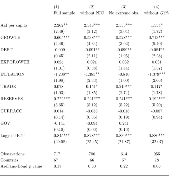
Column 1 of Table 1 presents the results of estimating (11).17 Most importantly,
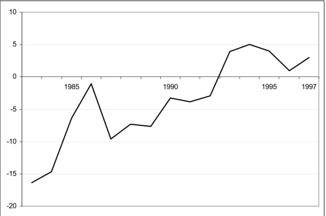
aid has a positive effect, and the coefficient is significant at the five percent level. Moreover, most control variables have the expected sign, although not all of them are significant. The coefficients of the time dummies, which are depicted in Figure 2 (but not reported in the table), also make sense, exhibiting a sharp drop during the debt crisis of the 1980s and a slow recovery during the 1990s.18 The probability value associated with the Arellano-Bond statistic
suggests that we can confidently reject the hypothesis that the disturbances are serially correlated. Finally, the results confirm the observation of Haque et al. (1996) that credit ratings are very persistent.19 On the one hand, this indicates
that creditworthiness is slow to react to a permanent increase of aid flows. On the
16This reduces the number of moment conditions since we have to lag the x-variables by at
leastthreeperiods to use them as instruments.
17These values are based on a one-step GMM estimator, which uses an exogenous weighting
matrix (see Arellano and Bond, 1991). While additional efficiency can be gained by deriving the weighting matrix in a two-step procedure, these gains are small relative to the lower reliability of the two-step estimator (see Bond, 2002:9).
18Note that the coefficients refer to the first-difference formulation in (11). Hence, a negative
value indicates that, on average, ratings decreased relative to the preceding year.
19However, the coefficient for the lagged dependent variable in Haque et al. (1996) is close
other hand, it implies that, although investor assessments return to some steady state level after a temporary “aid shock”, this convergence takes quite long and may buy a country time vis-a-vis international capital markets.
It is puzzling, though, that the ratio of debt over GDP is insignificant. This is in sharp contrast to preceding studies, which identified the debt level as a crucial determinant of perceived creditworthiness and interest rate spreads. A closer look at the data reveals that one single country may be responsible for this result: during the 1980s and 1990s, Nicaragua had debt levels way above the cross-country average, with a mind-boggling value of 1064 percent of GDP in 1990. In addition, the country experienced a hyperinflation in the late 1980s and current account deficits above 30 percent of GDP for several years in a row. While we have no reason to distrust these data, they show that the Nicaraguan experience is unusual in many dimensions. Put differently: our results so far may suffer from the fact that credit ratings just cannot be as bad as suggested by Nicaragua’s figures on inflation, external debt and current account deficits.
Our conjecture that the presence of Nicaragua in the sample distorts our find-ings is confirmed by column 2 in Table 1, which shows the results of estimating equation (11) without Nicaragua: the coefficient of debt is now significantly neg-ative. Moreover, trade openness has made it back into the club of significant regressors. Finally, aid continues to have a positive effect, now at the 1-percent level of significance.
Of course, Nicaragua is not the only country that experienced periods of ex-cessive inflation and indebtedness, and it could be argued that our results are driven by some other influential observation. In order to check this possibility, we removed countries that had annual inflation rates above 500 percent or debt levels above 200 percent of GDP for at least one year between 1980 and 2000. By setting these thresholds, we tried to strike a balance between our desire to eliminate “extreme” observations and the need to keep a reasonably large
sam-ple.20 We also removed Jordan, whose inflows of aid per capita in the 1980s
substantially exceeded those of other countries.21 Column 3 in Table 1 shows
that, quite surprisingly, this reduction of the sample – all in all, we sacrificed 92 observations – leaves the coefficient and the significance level of aid almost un-changed. Moreover, debt continues to have a negative effect. The inflation rate ceases to be significant, which confirms a standard result from empirical growth research: while hyperinflations definitely have a detrimental effect on growth, it is much harder to identify a significant role of price stability if one considers only countries with moderate inflation rates.22
To summarize: it appears that the presence of Nicaragua in the sample is quite important for the coefficients of some regressors – though not for the coefficient of aid –, whereas it does not really matter whether we include or exclude other “extreme observations”. In what follows, we will therefore work with a sample that discards the observations for Nicaragua, but includes all other countries.
In Section 3.1.3 we pointed out that the use of the “institutional” variable
GOVas a regressor shortens the time series in our panel since the IRIS III data set only covers the years between 1982 and 1997. Due to first-differencing and our decision to lag all regressors by one period, the regressions including GOV
thus only used observations for the years 1984 to 1998. Column 4 in Table 1 gives the results from estimating (11) without the governance variable, which allows us to use IICT observations between 1982 and 2000. Most notably, aid still has a positive effect on IICT, but the coefficient drops substantially, and the significance level increases to 8.5 percent.23 What explains the drop in the coefficient and the 20The countries that satisfy the above criteria are Argentina, Bolivia, Brazil, Congo,
Nicaragua, Peru, Poland, Russia, Mozambique, Ukraine, and Zambia.
21Between 1980 and 1990, per capita aid received by Jordan was usually more than five times
the cross-sectional average.
22See Fischer (1993), Barro (1995), Bruno and Easterly (1998), as well as Khan and Senhadji
(2001) for a more recent analysis.
hy-t-statistic for our aid variable? By re-estimating equation (11) withoutGOV, but with time series of varying length, we found that the result is mainly driven by the inclusion of the periods 1982-83, i.e. the years in which investor confidence was heavily shocked by Mexicos’s default and the resulting debt crisis.24 While
these observations do not invalidate our previous results, they suggest that aid may be less effective in supporting creditor confidence during times of extreme stress, when ratings are affected by rapidly deteriorating fundamentals and a general feeling of heightened uncertainty.
This important insight notwithstanding, we will return to our original speci-fication, which includesGOV as a regressor. The main reason is that, as we will see below, this variable has a significant effect on IICT for certain countries and time periods. Moreover, while using GOVas a regressor discards some informa-tion on the effects of aid during the tumultuous early 1980s and late 1990s, the shorter panel allows us to more clearly identify the impact of aid during periods of relative financial stability.25
3.3
Robustness checks
In this subsection, we will report the results from replacing ODA per capita in equation (11) by different types of aid, from running this regression for various country groups and time periods, and from experimenting with non-linear
spec-pothesis of serial correlation.
24A regression without GOVand without the observations for 1982-83 uses 882 data points
and yields a coefficient of 1.82, a t-statistic of 2.25, and an Arellano-Bond p-value of 0.13. The fit of our model further improves if we also exclude the years 1999-2000, i.e. the aftermath of the Asian crisis and the Russian default. In this case, we use 759 observations, the coefficient of aid is 2.52, while the t-statistic and the Arellano-Bond p-value rise to 3.26 and 0.33, respectively.
25Of course, GOV is not the only control variable whose inclusion reduces the size of our
sample. Hence, to be sure that our results are not an artifact of (non-deliberate) data-mining, we ran a regression with aid as the only regressor (in addition to time dummies). This regression, which was based on 1309 observations, yielded an aid coefficient of 5.47 and a t-statistic of 4.20.
ifications. Apart from testing the robustness of our findings, these variations provide important insights on the channels through which aid affects country creditworthiness.
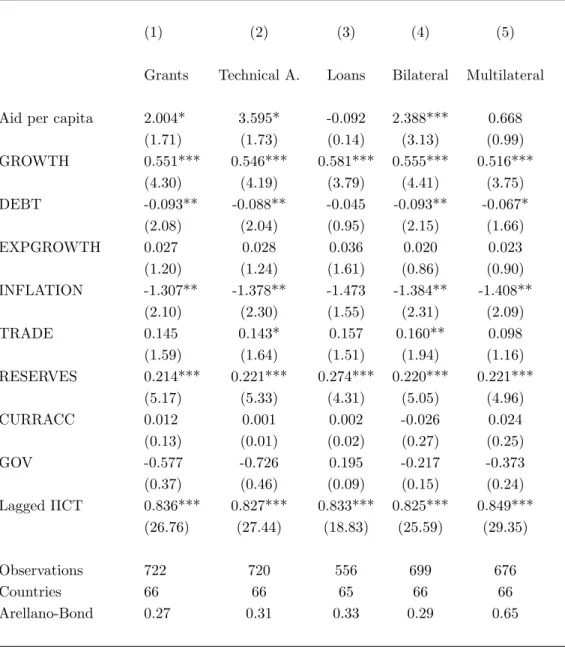
Table 2 differentiates between various types of aid: column 1 considers only
pure grants, while columns 2 and 3 consider technical assistance and loans, re-spectively. The other regressors are only marginally affected by this modification. However, while grants and technical assistance have a significantly positive effect on creditworthiness, the coefficient for loans is negative and not significant. This seems intuitive: both grants and technical assistance correspond to the type of transfer modelled in Section 2, with technical assistance being more likely to be used productively and to raise future income. Moreover, by establishing a long-term relationship between donor and recipient country, technical assistance expands the set of possible sanctions in case of default. Conversely, loans that raise the future debt burden seem to be unable to improve a country’s standing vis-a-vis international capital markets, even in the short run. Columns 4 and 5 of Table 2 show that bilateral aid has a much stronger impact on creditworthiness than multilateral aid. This may reflect the fact that multilateral aid frequently signals situations of financial emergency, which would have a negative impact on credit ratings. A second, complementary explanation for the stronger effect of bilateral aid is based on the notion that creditworthiness depends on the expected costs of default: multilateral aid may be less effective in raising these costs, since institutions like the World Bank and the IMF are less credible to sanction default than individual donor countries.
While grants and technical assistance are usually positive, there are several countries where net loans were negative for some years, i.e. in which repayments exceeded new disbursements. Since we are using logarithms, these observations necessarily drop out, and the size of our sample therefore decreases substantially. To make sure that this is not driving our results, we re-estimated equation (11) using aid over GDP as regressor. The first column of Table 3 demonstrates
that, with this specification, aid still has a significantly positive effect on country creditworthiness. Interestingly, this now also applies to all of its components – including loans and multilateral aid. However, as in Table 2, the effect of grants and technical assistance is still much stronger than the impact of loans. On the other hand, multilateral aid now seems to have a greater impact than bilateral aid. The reason for this striking difference to our results in Table 2 may be the fact that the log-transformation compresses the very large observations in our sample while a mere division by GDP does not, and that a few influential observations are thus driving the results in columns (5) and (6) of Table 3. To test this conjecture, we removed the series for Jordan – a country which received huge flows of bilateral aid in the 1980s – and re-ran the previous regressions. The coefficient of multilateral aid (as a share of GDP) fell to 0.60 (t-statistic: 1.65) while the coefficient of bilateral aid increased to 0.52 (t-statistic: 2.44). This partly re-establishes our previous result.
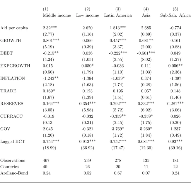
Table 4splits the sample into middle-income and low-income countries, and
along regional dimensions.26 Columns 1 and 2 demonstrate that aid has a
signif-icant effect for middle-income countries, but not for low-income countries. This is surprising, since we expected aid to have a much greater impact in those coun-tries that rely most heavily on foreign donors. The fact that even large inflows of aid fail to improve creditworthiness suggests that the poorest countries are stig-matized by a bad reputation, which is hardly affected by rising aid or changing economic fundamentals. This explanation is further supported by the observa-tion that the t-statistics of most other regressors are very low, too, and that the coefficient of the lagged dependent variable is much higher than for the middle-income countries. When we look at individual regions, the results (columns 3 to 5 in Table 4) reveal that aid has a significant effect in Latin America, while it
26See section 5.2 in the data appendix for a breakdown of our sample into low-income and
is insignificant in Asia and Africa. Note also that the effect of the governance variable is significantly positive for the Latin American and Asian subsamples, suggesting that, during the past two decades, institutional reforms contributed to restoring investor confidence in these countries. On the other hand, the coef-ficient of GOV is not significant for Africa – possibly, because this variable does not exhibit much time variation in African countries.27 The poor performance of
aid and of most other regressors in the case of Africa confirms the notion that countries at the lower end of the international income distribution are stuck with their poor credit ratings, and that neither large inflows of aid nor exceptional growth is able to change this.28
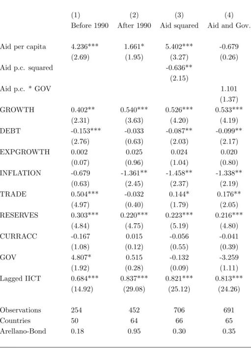
Columns 1 and 2 of Table 5report the results from running the regression for observations before and after 1990. While this break point is somewhat arbitrary, it is likely that aid disbursement criteria and thus the impact of aid changed after the end of the cold war. The numbers indicate that there are, indeed, substantial differences between the two decades: while the coefficients and t-statistics suggest a significantly positive effect in both periods, aid had a much stronger impact on credit ratings during the 1980s than during the 1990s. This may result from the fact that the number of low-income countries considered by theInstitutional Investorhas increased over the years. The weaker impact of aid in the 1990s may thus reflect the poor performance of aid in low-income countries. An alternative, less “mechanical” explanation is based on the observation that the average share of multilateral aid in total aid increased substantially between 1990 and 1998 (from 22 to 32 percent in our sample). Combined with our previous
27A possible explanation for the rather surprising negative coefficient of the current account
balance is that improving fundamentals may raise countries’ ability to attract foreign capital (and to finance current account deficits) before they are fully reflected by better credit ratings.
28Notably, export growth is one of the few significant determinants of creditworthiness for the
African and the low-income subsample. We interpret this finding as evidence of these countries’ dependence on raw materials exports.
result that multilateral aid is less effective in improving creditworthiness than bilateral aid, this may explain why both the coefficient and the t-statistic of aid are much lower in the 1990s.29 Note also that the role of debt, inflation, trade
openness, and institutional reform varies considerably between the “lost decade” and the “roaring nineties”: this may reflect both developing countries’ progress in liberalizing trade and improving the institutional framework and the shift of investors’ attention towards other hazards like low growth and high inflation.
We also investigated the proposition brought forward by Hansen and Tarp (2000) (among others) that there are diminishing returns to aid, and used the squared value of aid as an additional regressor. The numbers in column 3 of Table 5 support this idea: while the other coefficients are unaffected by the in-clusion of the nonlinear term, the coefficients of aid and aid squared suggest that aid flows above 70 US dollars per capita have a negative effect on creditworthi-ness – possibly because excessive aid dependence sends a bad signal to foreign investors.30
Finally, we checked whether the effect of aid on creditworthiness depends on the institutional environment and therefore included an interactive term – the logarithm of aid times our “institutional variable”GOV– as an additional regres-sor.31 As column 4 of Table 5 demonstrates, the notion that “money matters – in
a good policy environment” (World Bank, 1998:28) is not supported in our con-text: while the effects of aid on creditworthiness may be nonlinear, the marginal effect does not depend on the quality of institutions in recipient countries.
29We also checked whether the structural break was driven by a changing composition of aid
in terms of grants vs. loans. However, this conjecture was not supported by the data. In fact, the data reveal that the share of loans in total aiddecreasedthroughout the 1990s.
30Only few countries in our sample persistently passed this threshold.
31We excluded Nigeria whose per-capita aid inflows are frequently below one dollar. The log
transformation would have turned these observations into strongly negative values, and this would have distorted our results.
4
Summary and conclusions
When we started this investigation, we were curious whether aid could possi-bly raise developing countries’ creditworthiness and thus act as a “catalyst” for private capital flows. In this respect, our results are both encouraging and dis-heartening: aid raises the Institutional Investor’s index of country credit risk, but this effect seems to be limited to the subset of middle-income countries. By contrast, aid does not improve the reputation of low-income countries whose per-sistently low ratings keep deterring potential lenders. It is hard to decide whether this “debt intolerance” (Reinhart et al., 2003) is due to the inertia of investor expectations or due to entrenched institutional failure in these countries. Most likely it is both.
We also found some evidence that there are diminishing returns to aid: once aid (per capita) exceeds a certain level, additional inflows are counterproductive. On the other hand, there is no support for the notion that the marginal effect of aid on creditworthiness depends on the institutional environment in developing countries.
Finally, our results shed light on the channels through which aid may im-prove creditworthiness: technical cooperation seems to be more effective than pure grants or loans, suggesting that aid improves a country’s reputation when it raises future income and its potential losses from default. This conjecture is also supported by the observation that bilateral aid has a stronger impact on the
Institutional Investor’s ratings than multilateral aid. On a more general level, our results thus emphasize the importance to disentangle the different components of aid when assessing the effect of aid on macroeconomic variables. While this paper has limited its attention to the relationship between aid flows and credit-worthiness, we are quite sure that this insight generalizes to other parts of the aid-effectiveness debate.
References
Aizenman J.: “Country Risk, Asymmetric Information and Domestic Policies.”
NBER Working Paper 1880, (1986).
Aizenman J.: “Country Risk and Contingencies.”NBER Working Paper 2236,
(1987).
Alesina A. and D. Dollar: “Who Gives Foreign Aid to Whom and Why?”
Journal of Economic Growth ,vol. 5, 33-63, (2000).
Arellano M. and S. Bond: “Some Tests of Specification for Panel Data: Monte
Carlo Evidence and an Application to Employment Equations.” Review of Economic Studies, vol. 58, 277-297, (1991).
Barro R.: “Inflation and Economic Growth.” National Bureau of Economic
Research Inc., Working Paper 5326, (1995).
Bond S.: “Dynamic Panel Data Models: A Guide to Micro Data Methods and
Practice.” CEMMAP Working Paper No. CWP09/02, (2002).
Bruno M. and W. Easterly: “Inflation Crises and Long-Run Growth.”Journal
of Monetary Economics, vol. 41, 3-26, (1998).
Cantor R. and F. Packer: “Determinants and Impact of Sovereign Credit
Ratings.”FRBNY Economic Policy Review, (October 1996).
Chang C., E. Fernandez-Arias, and L. Serven: “Measuring Aid Flows: A
New Approach.” World Bank, Development Research Group, Washington D.C. , (1998).
Ciocchini F. and E. Durbin and D. Ng: “Does Corruption Increase Emerging
Market Bond Spreads?” Journal of Economics and Business, vol. 55, 503-28, (2003).
Cunningham, A., L. Dixon, and S. Hayes: “Analysing yield spreads on emerging market sovereign bonds” Bank of England Financial Stability Re-view, December 2001, 175-186., (2001).
Easterly W.: “Can Foreign Aid Buy Growth?” Journal of Economic
Perspec-tives, vol. 17, 23-48, (2003).
Easterly W., R. Levine, and D. Roodman: “New Data, New Doubts: A
Comment on Burnside and Dollar’s ”Aid, Policies, and Growth” (2000).”
The American Economic Review, forthcoming, (2003).
Eaton J., M. Gersovitz, and J. Stiglitz: “The Pure Theory of Country
Risk.”NBER Working Paper 1894, (1986).
Eichengreen B. and A. Mody: “What explains changing Spreads on Emerging
Market Debt: Fundamentals or Market Sentiment? ” NBER Working Paper No. 6408, (1998).
Fischer S.: “The Role of Macroeconomic Factors in Growth.” Journal of
Mon-etary Economics, vol. 32, 485-512, (1993).
Hansen H. and F. Tarp: “Aid effectiveness disputed.”Journal of International
Development, vol. 12, 375-398, (2000).
Hansen H. and F. Tarp: “Aid and growth regressions.” Journal of
Develop-ment Economics, vol. 64, 547-570, (2001).
Harms P. and M. Lutz: “Aid, Governance, and Private Foreign Investment:
Some Puzzling Findings and a Possible Explanation.” HWWA Discussion Paper 246, (2003).
Haque U. N., M. Kumar, N. Mark, and D. Mathieson: “The Economic Content of Indicators of Developing Country Creditworthiness.” IMF-Staff Papers, vol. 43, 688-724, (1996).
Haque U. N., N. Mark, and D. Mathieson: “The Relative Importance of
Political and Economic Variables in Creditworthiness Ratings.”IMF Work-ing Paper WP/98/46, (1998).
Jensen P and M. Paldam: “Can the new aid-growth models be replicated?”
Department of Economics, University of Aarhus, Working Paper No. 2003-17, (2003).
Judson R. and A. Owen: “Estimating Dynamic Panel Data Models: A Guide
for Macroeconomists” Economics Letters, vol. 65, 9-15, (1999).
Kahn M. and A. Senhadji: “Threshold Effects in the Relationship between
Inflation and Growth”IMF Staff Papers, vol. 48, 1-21, (2001).
Lee., M.: Panel data econometrics: methods-of-moments and limited dependent
variables, San Diego: Academic Press(1993).
Larrain F., H. Reisen, and J. von Maltzan: “Emerging Market Risk and
Sovereign Credit Ratings?” OECD Development Centre, Technical Paper No. 124, (1997).
Lee S.: “Are the credit ratings assigned by bankers based on the willingness
of LDC borrowers to repay?” Journal of Development Economics, vol. 40, 349-359, (1993).
Nickell S.: “Biases in Dynamic Models with Fixed Effects.” Econometrica, vol.
49, 1417-26, (1981)
Political Risk Services: International Country Risk Guide, (various issues).
Reinhart, C., K. Rogoff, and M. Savastano: “Debt Intolerance.”Brookings
Papers on Economic Activity, vol 0, no. 1, 2003, , 1-62, (2003).
Roodman, D. : “The Anarchy of Numbers: Aid, Development, and
Cross-country Empirics”Center for Global Development Working Paper 32, (2003).
Wooldridge J.: “Econometric Analysis of Cross Section and Panel Data.”
Cam-bridge, Massachusetts: The MIT Press, (2002).
World Bank: “Assessing aid: what works, what doesn’t, and why.” A World
Bank policy research report, Oxford University Press , (1998).
World Bank: “World Development Indicators on CD-ROM ”Washington DC,
The World Bank, (2003).
5
Data appendix
5.1
Definitions and sources
Institutional Investor Country Credit Rating (IICCR): Country Credit Ratings published in the Institutional Investor magazine every March and September since 1979. Source: Institutional Investor magazine, various issues.
Inflation: Annual percentage of inflation as measured by the consumer price index. Source: World Bank (2003).
Trade: Trade is the sum of exports and imports of goods and services measured as a share of gross domestic product. Source: World Bank (2003).
Debt: Total external debt divided by gross domestic product. Source: World Bank (2003).
Reserves: Net international reserves (excludes gold) divided by imports of goods and services. Source: World Bank (2003).
on constant local currency. World Bank (2003).
Current account balance: Current account balance is the sum of net exports of goods, services, net income, and net current transfers as percentage of gross domestic product. Source: World Bank (2003).
Export growth: Growth rate of exports of goods and services in current US dollars. Source: World Bank (2003).
Governance: Governance is an unweighted average of three International Country Risk Guide (ICRG) indices, ranging from 0 to 6: Corruption in Government: Lower scores indicate ”high government officials are likely to demand special payments” and that ”illegal payments are generally expected throughout lower levels of government” in the form of ”bribes connected with import and export licenses, exchange controls, tax assessment, police protection, or loans.”Rule of Law: This variable ”reflects the degree to which the citizens of a country are willing to accept the established institutions to make and implement laws and adjudicate disputes.” Higher scores indicate: ”sound political institutions, a strong court system, and provisions for an orderly succession of power.” Lower scores indicate: ”a tradition of depending on physical force or illegal means to settle claims.” Upon changes in government new leaders ”may be less likely to accept the obligations of the previous regime.” Quality of the Bureaucracy: High scores indicate ”an established mechanism for recruitment and training,” ”autonomy from political pressure,” and ”strength and expertise to govern without drastic changes in policy or interruptions in government services” when governments change. Source: Political Risk Services
Aid: Official development assistance and net official aid (2001 US dollars). Source: OECD (2004).
Technical cooperation: Technical co-operation is the provision of know-how in the form of personnel, training, research and associated costs (2001 US dollars). Source: OECD (2004).
Grants: Grants are transfers in cash or in kind for which no legal debt is incurred by the recipient (2001 US dollars). OECD (2004).
debt (2001 US dollars). OECD (2004).
Bilateral Aid: Bilateral transactions are those undertaken by a donor country directly with an aid recipient (2001 US dollars). Source: OECD (2004).
Multilateral Aid: Total net aid flows minus bilateral aid (2001 US dollars). Source: OECD (2004).
5.2
Countries in the sample
Algeria, (Angola*), Argentina, Bangladesh*, (Benin*), Bolivia, Botswana, Brazil, Bul-garia, Burkina Faso*, Cameroon*, Chile, China, Colombia, Congo Rep.*, Costa Rica, Cote d’Ivoire*, (Croatia), Dominican Republic, Ecuador, Egypt Arab Rep., El Sal-vador, (Estonia), Ethiopia*, Gabon, (Georgia*), Ghana*, Guatemala, Haiti*, Hon-duras, Hungary, India*, Indonesia*, Jamaica, Jordan, (Kazakhstan), Kenya*, (Latvia), (Lithuania), Malawi*, Malaysia, Mali*, (Mauritius), Mexico, Morocco, Mozambique*, (Nepal*), Nicaragua*, Nigeria*, Oman, Pakistan*, Panama, Papua New Guinea*, Paraguay, Peru, Philippines, Poland, Romania, Russian Federation, Senegal*, Sierra Leone*, South Africa, Sri Lanka, Sudan*, Syrian Arab Republic, Tanzania*, Thai-land, Togo*, Trinidad and Tobago, Tunisia, Turkey, Uganda*, (Ukraine*), Uruguay, Venezuela RB, Vietnam*, Zambia*, Zimbabwe*.
Note: Low-income countries, i.e. countries in which 2001 GNI per capita was 745 US dollars or less (World Bank 2003), are marked with an asterisk. Countries in brackets ar those used only in regression (4) of Table 1.
5.3
Summary statistics
Mean Max. Min. Std. Dev. Skewness Kurtosis IICCR 28.00 68.85 4.35 13.76 0.64 2.96 IICT -105.89 79.31 -309.05 74.91 -0.12 2.84
Aid per capita 35.48 468.26 -18.61 41.86 3.58 26.78 Techn.ass. p.c. 9.01 67.23 -9.27 8.61 2.17 10.35 Grants p.c. 27.12 416.89 0.36 35.20 4.25 33.98 Loans p.c. 8.36 140.70 -85.10 15.96 0.79 16.98 Multilat. aid p.c. 8.16 61.76 -25.40 9.41 1.65 7.00 Bilat. aid p.c. 27.32 453.40 -18.80 37.72 4.46 36.99 Aid/GDP 5.40 78.94 -0.55 8.01 3.30 20.00 Techn. ass./GDP 1.19 11.33 -0.30 1.53 2.57 12.21 Grants/GDP 3.94 49.67 0.01 6.06 3.23 17.37 Loans/GDP 1.45 29.27 -10.60 2.68 3.07 24.30 Multil. aid/GDP 1.78 24.48 -0.76 3.33 3.17 14.88 Bilat. aid/GDP 3.62 54.46 -0.46 5.22 3.65 24.49 GROWTH 1.22 16.54 -20.90 4.72 -0.77 5.29 DEBT 74.72 339.21 7.40 49.50 1.86 7.85 EXPGROWTH 9.16 283.76 -79.44 21.48 3.58 42.69 INFLATION 82.99 11749.64 -11.69 568.90 15.38 280.01 TRADE 58.27 192.11 12.35 27.58 1.12 5.37 RESERVES 27.38 276.91 0.04 29.06 4.35 32.80 CURRACC -3.77 28.71 -44.84 6.37 -1.25 11.58 GOV 2.85 5.33 0.67 0.86 -0.20 2.95
Annotations: The summary statistics refer to the 66 countries on which regression (2) in Table 1 is based.
6
Tables
Table 1: Aid and country creditworthiness
(Dependent variable: Transformed index of country credit risk)
(1) (2) (3) (4)
Full sample without NIC No extreme obs. withoutGOV
Aid per capita 2.262** 2.548*** 2.533*** 1.534*
(2.49) (3.12) (3.04) (1.72) GROWTH 0.605*** 0.538*** 0.528*** 0.713*** (4.46) (4.34) (3.92) (5.40) DEBT -0.009 -0.091** -0.099** -0.084** (0.45) (2.11) (1.95) (2.28) EXPGROWTH 0.025 0.021 0.032 0.031 (1.01) (0.88) (1.44) (1.37) INFLATION -1.208** -1.383** -0.810 -1.379*** (1.98) (2.33) (1.00) (2.66) TRADE 0.078 0.151* 0.219*** 0.117* (1.03) (1.85) (2.74) (1.78) RESERVES 0.222*** 0.221*** 0.241*** 0.192*** (5.65) (5.12) (5.22) (5.20) CURRACC 0.014 -0.035 -0.018 -0.087 (0.14) (0.36) (0.19) (0.94) GOV -0.141 -0.094 0.241 (0.10) (0.06) (0.16) Lagged IICT 0.845*** 0.828*** 0.839*** 0.880*** (29.08) (25.45) (21.87) (32.07) Observations 717 706 614 955 Countries 67 66 57 78 Arellano-Bondpvalue 0.17 0.30 0.22 0.03
Notes: In parentheses: Absolute values oft-statistics, based on a robust covariance-matrix.
**, **, *: significance levels of 1, 5, 10 percent.
Column (2): Sample without observations for Nicaragua.
Column (3): Sample without observations for Argentina, Bolivia, Brazil, Nicaragua, Peru, Poland, Russia, Ukraine, Congo, Mozambique, Zambia, Jordan.
All regressors are lagged by one period. All regressions include time dummies.
Table 2: Different types of aid
(Dependent variable: Transformed index of country credit risk)
(1) (2) (3) (4) (5)
Grants Technical A. Loans Bilateral Multilateral
Aid per capita 2.004* 3.595* -0.092 2.388*** 0.668
(1.71) (1.73) (0.14) (3.13) (0.99) GROWTH 0.551*** 0.546*** 0.581*** 0.555*** 0.516*** (4.30) (4.19) (3.79) (4.41) (3.75) DEBT -0.093** -0.088** -0.045 -0.093** -0.067* (2.08) (2.04) (0.95) (2.15) (1.66) EXPGROWTH 0.027 0.028 0.036 0.020 0.023 (1.20) (1.24) (1.61) (0.86) (0.90) INFLATION -1.307** -1.378** -1.473 -1.384** -1.408** (2.10) (2.30) (1.55) (2.31) (2.09) TRADE 0.145 0.143* 0.157 0.160** 0.098 (1.59) (1.64) (1.51) (1.94) (1.16) RESERVES 0.214*** 0.221*** 0.274*** 0.220*** 0.221*** (5.17) (5.33) (4.31) (5.05) (4.96) CURRACC 0.012 0.001 0.002 -0.026 0.024 (0.13) (0.01) (0.02) (0.27) (0.25) GOV -0.577 -0.726 0.195 -0.217 -0.373 (0.37) (0.46) (0.09) (0.15) (0.24) Lagged IICT 0.836*** 0.827*** 0.833*** 0.825*** 0.849*** (26.76) (27.44) (18.83) (25.59) (29.35) Observations 722 720 556 699 676 Countries 66 66 65 66 66 Arellano-Bond 0.27 0.31 0.33 0.29 0.65
Notes: In parentheses: Absolute values oft-statistics, based on a robust covariance-matrix.
**, **, *: significance levels of 1, 5, 10 percent. All regressors are lagged by one period. All regressions include time dummies.
Table 3: Aid as percentage of GDP
(Dependent variable: Transformed index of country credit risk)
(1) (2) (3) (4) (5) (6)
Total Aid Grants Technical A. Loans Bilateral Multilateral
Aid / GDP 0.413** 0.447** 3.909*** 0.342* 0.430** 0.711* (2.52) (2.36) (3.38) (1.85) (1.99) (1.86) GROWTH 0.605*** 0.582*** 0.562*** 0.583*** 0.597*** 0.579*** (4.53) (4.50) (4.29) (4.37) (4.48) (4.39) DEBT -0.119** -0.106** -0.142*** -0.106** -0.108** -0.114*** (2.55) (2.42) (3.44) (2.28) (2.31) (2.63) EXPGROWTH 0.028 0.028 0.032 0.029 0.029 0.027 (1.16) (1.22) (1.40) (1.26) (1.24) (1.15) INFLATION -1.261** -1.330** -1.233** -1.282** -1.284** -1.343** (2.09) (2.16) (2.15) (2.03) (2.08) (2.15) TRADE 0.137 0.135 0.145 0.144 0.134 0.151 (1.49) (1.49) (1.61) (1.52) (1.44) (1.63) RESERVES 0.211*** 0.216*** 0.229*** 0.217*** 0.214*** 0.215*** (5.21) (5.35) (5.50) (5.23) (5.30) (5.27) CURRACC 0.028 0.024 -0.042 0.004 0.017 0.015 (0.28) (0.25) (0.40) (0.04) (0.17) (0.14) GOV -0.318 -0.389 -0.725 -0.575 -0.583 -0.193 (0.20) (0.25) (0.47) (0.36) (0.37) (0.13) Lagged IICT 0.835*** 0.833*** 0.821*** 0.840*** 0.836*** 0.833*** (26.10) (26.56) (26.97) (27.31) (26.27) (26.61) Observations 722 722 722 722 722 722 Countries 66 66 66 66 66 66 Arellano-Bond 0.27 0.30 0.46 0.28 0.26 0.33
Notes: In parentheses: Absolute values oft-statistics, based on a robust covariance-matrix.
**, **, *: significance levels of 1, 5, 10 percent. All regressors are lagged by one period. All regressions include time dummies.
Table 4: Low- vs. middle income countries and regional differences
(Dependent variable: Transformed index of country credit risk)
(1) (2) (3) (4) (5)
Middle income Low income Latin America Asia Sub.Sah. Africa
Aid per capita 2.32*** 2.620 1.813*** 2.685 -0.774
(2.77) (1.16) (2.02) (0.89) (0.37) GROWTH 0.801*** 0.066 0.457*** 0.681** 0.161 (5.19) (0.39) (3.37) (2.00) (0.88) DEBT -0.215** 0.036 -0.222*** -0.501*** 0.049 (4.24) (1.05) (3.55) (8.02) (1.27) EXPGROWTH 0.015 0.050* -0.036 0.111 0.056** (0.50) (1.79) (1.10) (1.03) (2.36) INFLATION -1.243** -1.364 -1.039* 0.374 -1.397 (2.18) (1.63) (1.74) (0.28) (1.56) TRADE 0.169* 0.123 0.195 0.057 0.148 (1.67) (1.39) (1.51) (0.61) (1.46) RESERVES 0.164*** 0.354*** 0.292*** 0.332*** 0.281*** (3.05) (5.98) (5.72) (6.92) (3.06) CURRACC -0.019 -0.032 -0.359** -0.359* 0.026 (0.13 (0.31) (2.45) (1.75) (0.20) GOV 2.045 -0.321 3.769* 5.260* 1.237 (1.20) (0.18) (1.72) (1.84) (0.49) Lagged IICT 0.754*** 0.913*** 0.752*** 0.684*** 0.92*** (18.99) (36.92) (17.47) (12.30) (39.16) Observations 467 239 278 135 181 Countries 40 26 20 11 22 Arellano-Bond 0.24 0.52 0.67 0.07 0.24
Notes: In parentheses: Absolute values oft-statistics, based on a robust covariance-matrix.
**, **, *: significance levels of 1, 5, 10 percent. All regressors are lagged by one period. All regressions include time dummies.
Table 5: Structural breaks and nonlinear effects
(Dependent variable: Transformed index of country credit risk)
(1) (2) (3) (4)
Before 1990 After 1990 Aid squared Aid and Gov.
Aid per capita 4.236*** 1.661* 5.402*** -0.679
(2.69) (1.95) (3.27) (0.26) Aid p.c. squared -0.636** (2.15) Aid p.c. * GOV 1.101 (1.37) GROWTH 0.402** 0.540*** 0.526*** 0.533*** (2.31) (3.63) (4.20) (4.19) DEBT -0.153*** -0.033 -0.087** -0.099** (2.76) (0.63) (2.03) (2.17) EXPGROWTH 0.002 0.025 0.024 0.020 (0.07) (0.96) (1.04) (0.80) INFLATION -0.679 -1.361** -1.458** -1.338** (0.63) (2.45) (2.37) (2.19) TRADE 0.504*** -0.032 0.144* 0.176** (4.97) (0.40) (1.79) (2.05) RESERVES 0.303*** 0.220*** 0.223*** 0.216*** (4.84) (4.75) (5.19) (4.80) CURRACC -0.167 0.015 -0.056 -0.041 (1.08) (0.12) (0.55) (0.39) GOV 4.807* 0.515 -0.132 -3.259 (1.92) (0.28) (0.09) (1.11) Lagged IICT 0.684*** 0.837*** 0.821*** 0.813*** (14.92) (29.08) (25.12) (24.26) Observations 254 452 706 691 Countries 50 64 66 65 Arellano-Bond 0.18 0.95 0.30 0.35
Notes: In parentheses: Absolute values oft-statistics, based on a robust covariance-matrix.
**, **, *: significance levels of 1, 5, 10 percent. All regressors are lagged by one period. All regressions include time dummies.
6 -u0(A 1) u0(Y 2) D2 D∗ 2
-20 -15 -10 -5 0 5 10 1985 1990 1995 1997