Partially evaluating finite-state runtime monitors ahead of time
ERIC BODDEN, Technische Universit¨at DarmstadtPATRICK LAM, University of Waterloo
LAURIE HENDREN, McGill University
Finite-state properties account for an important class of program properties, typically related to the order of operations invoked on objects. Many library implementations therefore include manually-written finite-state monitors to detect violations of finite-state properties at runtime. Researchers have recently proposed the explicit specification of finite-state properties and automatic generation of monitors from the specification. However, runtime monitoring only shows the presence of violations, and typically cannot prove their absence. Moreover, inserting a runtime monitor into a program under test can slow down the program by several orders of magnitude.
In this work, we therefore present a set of four static whole-program analyses that partially evaluate runtime monitors at compile time, with increasing cost and precision. As we show, ahead-of-time evaluation can often evaluate the monitor completely statically. This may prove that the program cannot violate the property on any execution or may prove that violations do exist. In the remaining cases, the partial evaluation converts the runtime monitor into a residual monitor. This monitor only receives events from program locations that the analyses failed to prove irrelevant. This makes the residual monitor much more efficient than a full monitor, while still capturing all property violations at runtime.
We implemented the analyses inClara, a novel framework for the partial evaluation of AspectJ-based runtime monitors, and validated our approach by applying Clarato finite-state properties over several large-scale Java programs.Claraproved that most of the programs never violate our example properties. Some programs required monitoring, but in those casesClaracould often reduce the monitoring overhead to below 10%. We observed that several programs did violate the stated properties.
Categories and Subject Descriptors: D.2.4 [Software Engineering]: Software/Program Verification— Val-idation
General Terms: Algorithms, Experimentation, Performance, Verification
Additional Key Words and Phrases: typestate analysis, static analysis, runtime monitoring 1. INTRODUCTION AND CONTRIBUTIONS
Finite-state properties constrain acceptable operations on a single object or a group of inter-related objects, depending on the object’s or group’s history. Typestate systems [Strom and Yemini 1986], an instantiation of the idea of finite-state properties, enable the specification and (potentially static) verification of finite-state properties for program understanding and verification. One can define type systems [Bierhoff and Aldrich 2007; DeLine and F¨ahndrich 2004] that prevent programmers from writing code with typestate errors. Unfortunately, current typestate systems require elaborate program annotations, essentially to identify statements that may access an object (and hence modify its typestate) and variables that may or must point to the same objects (i.e., may or must alias). Such annotations are hard to maintain, possibly explaining in part why such type systems have not been adopted.
Portions of this work were published in [Bodden et al. 2007; Bodden et al. 2008a; Bodden 2010; Bodden et al. 2010].
Permission to make digital or hard copies of part or all of this work for personal or classroom use is granted without fee provided that copies are not made or distributed for profit or commercial advantage and that copies show this notice on the first page or initial screen of a display along with the full citation. Copyrights for components of this work owned by others than ACM must be honored. Abstracting with credit is permitted. To copy otherwise, to republish, to post on servers, to redistribute to lists, or to use any component of this work in other works requires prior specific permission and/or a fee. Permissions may be requested from Publications Dept., ACM, Inc., 2 Penn Plaza, Suite 701, New York, NY 10121-0701 USA, fax +1 (212) 869-0481, or [email protected].
c
YYYY ACM 0164-0925/YYYY/01-ARTA $10.00
connected disconnected error CLOSE RECONNECT CLOSE, RECONNECT, WRITE WRITE CLOSE WRITE
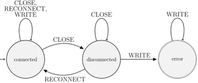
Fig. 1: “ConnectionClosed” finite-state property: no write after close.
A more pragmatic approach is to instead monitor programs for violations of finite-state properties at runtime. Several researchers have proposed notations and tools to support monitoring for finite-state properties expressed using tracematches or other formalisms [Al-lan et al. 2005; Bodden 2005; Chen and Ro¸su 2007; Maoz and Harel 2006; Kr¨uger et al. 2006]. The tracematches formalism combines regular expressions with AspectJ [Kiczales et al. 2001] pointcuts to provide a high-level specification language for runtime monitors. JavaMOP [Chen and Ro¸su 2007] is an open framework for notations that can generate monitors from high-level specifications written in different concrete notations such as lin-ear temporal logic, regular expressions or context-free grammars. Runtime monitoring is appealing because monitor specifications can be very expressive: they can reason about concrete program events and concrete runtime objects, and thus completely avoid false warnings. However, runtime monitoring basically amounts to testing, where the runtime monitor merely provides a principled way to insert high-level assertions into the program under test. Testing, however, has several drawbacks. A suite of sufficiently varying test runs may be able to identify errors or strengthen a programmer’s confidence in her program by not identifying errors, but it does not constitute a correctness proof if the test suite is not complete. Secondly, runtime monitoring requires program instrumentation, and, as we show in this paper, this instrumentation may slow down the program under test by several orders of magnitude, making exhaustive testing even less of an option in many cases.
In this work we therefore propose a hybrid approach that starts with a runtime monitor but then uses static analysis results to convert this monitor into a residual runtime monitor. The residual monitor captures actual property violations as they occur, but updates its internal state only at relevant statements, as determined through static analysis. Unlike static type systems, our approach requires no program annotations; it is fully automatic. Program annotations for state changes are replaced by non-intrusive AspectJ pointcuts. Program annotations for aliasing constraints are not necessary in our approach because we infer aliasing constraints through a combination of precise pointer analyses.
Static analyses for optimizing monitors have different requirements from fully-static ap-proaches. Consider our running example, in which programmers must not write to a connec-tion handle that is currently in its “disconnected” state. Figure 1 shows a non-deterministic finite-state machine for this property. It monitors a connection’s CLOSE, RECONNECT and WRITE events and signals an error at its accepting state. (The looping transitions on the initial state implement our matching semantics, where the runtime monitor signals an error each time it reaches a final state. Because the machine is non-deterministic, the self-loops shown in the figure enable the monitor to report more than one violation for a single runtime trace.) A correct runtime monitor must observe events like CLOSE and WRITE that can cause a property violation, but also events like RECONNECT that may prevent the violation from occurring. Missing the former causes false negatives while missing the latter causes false positives, i.e., false warnings. Both are unacceptable, so our approach guarantees that executions of the generated monitor have no false positives or false negatives—it may
do so by deferring some decisions until runtime. Sound static approaches that only attempt to prove the absence of property violations but have no runtime monitoring component, e.g. [Fink et al. 2006], have no such option; deferring decisions is not acceptable. They can only declare false positives.
We present a set of four static analysis algorithms that evaluate finite-state runtime moni-tors ahead of time, with increasing precision. All algorithms analyze so-calledshadows [Ma-suhara et al. 2003]. The term “shadows” is popular in the aspect-oriented programming community and refers to program locations that can trigger runtime events of interest. The first analysis, the Quick Check, uses simple syntactic checks only. In our example, the Quick Check may be able to infer that a program opens and closes connections but never writes to a connection. Such a program cannot violate the property—if there are no writes, then no write can ever follow a close operation. The second analysis stage, the Orphan-shadows Analysis, applies a similar check on a per-object basis. If a program opens and closes some connectionc, but never writes toc, then the analysis can rule out violations onc(but not on other connections, based on this information). This stage uses points-to analysis to handle aliasing, i.e., to decide whether or not two variables may point to the same runtime connec-tion object. The third stage, the Nop-shadows Analysis, takes the program’s control-flow into account. Using a backward analysis, it first computes, for every transition statements
(e.g. statements causing events of type CLOSE, RECONNECT or WRITE), sets of states that are, ats, equivalent with respect to all possible continuations of the control flow fol-lowing s. The analysis then uses a forward pass to find transition statements that only switch between equivalent states. Switching between equivalent states is unnecessary, and the analysis removes such transitions.
As we prove, all three analysis stages are sound, i.e., when an analysis asserts that a program location requires no monitoring, then removing transitions from that location will never alter the program locations at which the runtime monitor will (or will not) reach its er-ror state. However, all three analyses are also incomplete: they may fail to identify program locations that actually require no monitoring. We therefore investigated and developed a fourth analysis, the Certain-match Analysis, which reports no false positives but may miss actual violations. This analysis is thus similar in flavour to unsound static checkers as im-plemented, for instance, in FindBugs [Hovemeyer and Pugh 2004] or PMD [Copeland 2005]. The Certain-match Analysis applies the same forward pass as the Nop-shadows Analysis, but instead identifies program locations at which the program certainly triggers a prop-erty violation. Such certain matches help programmers find true positives in a larger set of potential false positives.
We have implemented our analyses in Clara (CompiLe-time Approximation of Run-time Analyses), our novel framework for partially evaluating runRun-time monitors ahead of time [Bodden et al. 2010; Bodden 2010]. We developed Clara to facilitate the integra-tion of research results from the static analysis, runtime verificaintegra-tion and aspect-oriented-programming communities. Clara features a formally specified abstraction, Dependency State Machines, which function as an abstract interface, decoupling runtime monitors from their static optimizations. The analyses that we present in this paper therefore apply to any runtime monitor implemented as an AspectJ aspect that uses Dependency State Ma-chines. Our analyses are therefore compatible with a wide range of state-of-the-art runtime verification tools [Allan et al. 2005; Bodden 2005; Chen and Ro¸su 2007; Maoz and Harel 2006; Kr¨uger et al. 2006], if they are extended to produce Dependency State Machines. We ourselves have successfully used Clara in combination with tracematches and Java-MOP [Bodden et al. 2009; Bodden 2009].
To evaluate our approach, we applied the analysis to the DaCapo benchmark suite [Black-burn et al. 2006]. In our experiments, in 68% of all casesClara’s analyses can prove that the program is free of program locations that could drive the monitor into an error state. In these cases, Clarastatically guarantees that the program can never violate the stated
property, eliminating the need for runtime monitoring of that program. In other cases, the residual runtime monitor will require less instrumentation than the original monitor, there-fore yielding a reduced runtime overhead. For monitors generated from a tracematch [Allan et al. 2005] specification, in 65% of all cases that showed overhead originally, no overhead remains after applying the analyses. The Certain-match Analysis, on the other hand, does not appear to be very effective: in our benchmark set, it could only identify a single match
ascertain, even though our runtime monitors signal several matches at runtime. Due to the
design of our analyses and the Claraframework, our analyses are equally effective on any runtime monitor for a given property, independent of the source of the monitor.
To summarize, this paper presents the following contributions:
— A set of three static whole-program analyses that can partially evaluate finite-state mon-itors ahead of time, with increasing precision.
— Soundness proofs for those three analyses.
— A novel Certain-match Analysis that can determine inevitable property violations on an intra-procedural level.
— A system for presenting analysis results to the user to support manual code inspection in the Eclipse integrated development environment.
— An open-source implementation of these analyses in the context of theClaraframework and a large set of experiments that validates the effectiveness of our approach based on large-scale, real-world benchmarks drawn from the DaCapo benchmark suite.
The relationship of this article to previous publications is as follows. Two of the contri-butions in this article are entirely novel: the design, implementation, and evaluation of the Certain-match Analysis (Section 8), and the Eclipse plugin for presenting analysis results to developers (Section 9). This article also presents improved—more precise or faster—versions of two previously-presented static analyses for eliminating unnecessary monitoring points (see Section 11.3 for details), and presents a complete description of the Nop-shadows Anal-ysis (Section 7), for the first time, including its handling of pointers and inter-procedural effects. We have also improved the presentation of the soundness proofs for the static analy-ses from Bodden’s PhD thesis [2009]. In summary, this article presents a consolidated view of the entire Clara framework, notably including all of its static analyses, the relevant correctness proofs, and a full evaluation, in a single publication.
2. RUNNING EXAMPLE
We continue by presenting a specification for the ConnectionClosed finite-state property and explaining how our static analyses can analyze programs for conformance with this property. In particular, we will demonstrate how our analyses behave on code that always violates the property, code that sometimes violates the property, and code that never violates the property.
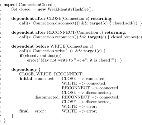
Recall that the ConnectionClosed property specifies that programs may not write to closed connections. Figure 2 presents a textual specification of the ConnectionClosed prop-erty using Dependency State Machines, Clara’s intermediate representation for runtime monitors. Specifications in Clara consist of an AspectJ aspect (implementing a runtime monitor for the property), augmented with additional annotations that aid static analysis. The example aspect consists of three pieces of advice (lines 4–13) which intercept disconnect, reconnect and write events. When disconnecting a connection, the CLOSE advice places the closed connection object into the setclosed. When the connection is re-connected, the RECONNECT advice removes it from the set again. Finally, the WRITE advice issues an error message upon any write to a connection in theclosedset. Note that the aspect uses its own data structure—the set in line 2—to keep track of closed connections.Claraseeks to be independent of such internal implementation details. The aspect therefore carries an additional,Clara-specific annotation in lines 15–25: the monitor’s Dependency State
Ma-1 aspectConnectionClosed{
2 Set closed =newWeakIdentityHashSet(); 3
4 dependent afterCLOSE(Connection c)returning:
5 call(∗ Connection.disconnect()) && target(c){closed.add(c);} 6
7 dependent afterRECONNECT(Connection c)returning:
8 call(∗ Connection.reconnect()) &&target(c){closed.remove(c);} 9
10 dependent beforeWRITE(Connection c): 11 call(∗ Connection.write (..)) &&target(c){ 12 if(closed . contains(c))
13 error (”May not write to ”+c+”: it is closed ! ” ); } 14
15 dependency{
16 CLOSE, WRITE, RECONNECT;
17 initial connected: CLOSE−>connected,
18 WRITE−>connected,
19 RECONNECT−>connected,
20 CLOSE−>disconnected;
21 disconnected: RECONNECT−>connected,
22 CLOSE−>disconnected,
23 WRITE−>error;
24 final error : WRITE−>error;
25 }
26 }
Fig. 2: “ConnectionClosed” aspect with Dependency State Machine.
chine. This state machine encodes the internal transition structure of the pieces of advice that implement the monitoring logic. Note that this is a textual representation of the state machine from Figure 1. We will formally define the semantics of Dependency State Machines in Section 4. [Bodden 2009] presents the formal syntax for these annotations.
The design of Dependency State Machines inClaraallows them to function as an ab-stract interface, bridging the efforts of the static analysis community to efforts of the runtime verification community. Many state-of-the-art runtime verification tools generate monitors in the form of AspectJ aspects, because such aspects offer a convenient and declarative way to define the program points which require instrumentation. Figure 3, for example, shows a high-level tracematch [Allan et al. 2005] specification for ConnectionClosed. Tracematches
1 aspectConnectionClosed{ 2 tracematch(Connection c){
3 symCLOSE after returning:call(∗Connection.disconnect()) &&target(c); 4 symRECONNECT after returning:call(∗Connection.reconnect()) &&target(c); 5 symWRITEafter returning:call(∗Connection.write(..)) &&target(c);
6
7 CLOSE+ WRITE{
8 error (”May not write to ”+c+”, as it is closed ! ” );
9 }
10 }
11 }
allow programmers to match on the execution history via a regular expression over AspectJ pointcuts. Line 2 states that the tracematch reasons about one connection c at a time. Lines 3–5 define the set of events that the monitor wishes to process. The events form sym-bols of an alphabet (hence the keyword sym), and line 7 uses this alphabet to define the regular expression “CLOSE+ WRITE”. The body (lines 7–9) will therefore execute after one or more disconnects, followed by a write, as long as there is no intervening reconnect. The tracematch implementation generates an AspectJ aspect similar to the one we showed in Figure 2 from this specification. Other runtime verification tools also generate similar aspects from their specification languages. By augmenting an aspect with a Dependency State Machine annotation, a tool can easily make its generated aspects available forClara to analyze and optimize. In our experiments, we will focus on optimizing runtime moni-tors from tracematches. However, in previous work [Bodden et al. 2009], we have shown that our analyses are equally effective on monitors generated from other types of high-level specifications. The only requirement forClara’s clients is that the provided Dependency State Machine annotations must be semantically equivalent to the annotated runtime mon-itor. In Section 4.1 we provide a full dynamic semantics of Dependency State Machines, which clients can use to prove that the provided Dependency State Machine annotations are indeed correct.
1 public static voidmain(String args[]){ 2 Connection c =newConnection(args[0]); 3 c . disconnect (); // CLOSE(c)
4 c . write(args [0]); // WRITE(c): violation−write after close on c 5 }
(a) Example program which always matches
1 public static voidmain(String args[]){ 2 Connection c1 =newConnection(args[1]),
3 c2 =newConnection(args[2]);
4 c1.disconnect (); // CLOSE(c1)
5 c2.write(args [0]); // WRITE(c2): write, but on c2, hence independent of 4 6 }
(b) Example program which never matches due to incompatibility of transitions
1 public static voidmain(String args[]){ 2 Connection c =newConnection(args[0]); 3 c . write(args [0]); // WRITE(c)
4 c . disconnect (); // CLOSE(c): no violation, since it always follows 3 5 }
(c) Example program which never matches due to ordering of transitions
1 public static voidmain(String args[]){ 2 Connection c =newConnection(args[0]), 3 if (args .length >1)
4 c . disconnect (); // CLOSE(c)
5 c . write(args [0]); // WRITE(c): violation−write after close possible 6 }
(d) Example program which matches on some inputs
Next, we discuss our analysis of ConnectionClosed on the code in Figure 4. Figure 4a always triggers the final state of the monitor, since it contains a connection close followed by a write on the same connection. Our Certain-match Analysis will determine that it always triggers the final state. It does so by performing a flow-sensitive propagation of possible states for the connection c; after line 2, the connection is in the initial “connected” state. Following the CLOSE and WRITE transitions, our analysis can deduce that the connection is sure to reach the final “error” state.
Our remaining analyses are staged: Clararuns a series of analyses in turn, from least computationally expensive to most expensive. The idea is to do as little work as possible to try to guarantee that programs do not violate properties. The first stage, Quick Check, therefore only collects the labels of transitions in the program, and eliminates the transitions which never affect whether or not the program triggers a final state. The second stage, Orphan-shadows Analysis, sharpens this information with pointer information. Finally, the third stage, Nop-shadows Analysis, is flow-sensitive: it uses information about the ordering of potential transitions in the program to rule out transitions which can never trigger the final state.Clarathen groups the remaining transitions intopotential failure groups, using points-to information: transitions that can potentially affect the same object appear in the same group. As we explain in Section 9, this eases manual code inspection.
Figure 4b presents one example of a program which never triggers the final transition. In this case, the program contains both WRITE and CLOSE transitions, so the Quick Check cannot remove these transitions. However, our pointer analysis finds that the connection objects c1 and c2 are distinct, so that no single object executes both the WRITE and CLOSE transition. The Orphan-shadows Analysis therefore instructs Clara to remove both transitions in Figure 4b.
Figure 4c also never triggers the final state, even though it contains all of the necessary transitions on appropriate objects. The analysis must track object abstractions through their potential states. In particular, our Nop-shadows Analysis establishes that the connection starts in its initial state after instantiation at line 2. Next, it follows the transitions in lines 3 and lines 4 to reason that these lines never trigger the monitor. Finally, since connectionc
does not escape themainmethod, the analysis can conclude that no other transition in the program affectsc, so that none of the transitions oncin themainmethod affect a possible match. Note that it is much harder to prove that transitions are unnecessary than that they are necessary (as we did for Figure 4a).
Finally, Figure 4d illustrates a program for which no static analysis can determine whether or not the final state is triggered, in this case because the transitions taken depend on program input. Each of our analyses would state that each transition could occur and has a potential effect on the state machine.
Parameterized traces.Every program run generates a parameterized trace [Chen and
Ro¸su 2009] over the pieces of advice applicable to that run. (The traces are parameterized by object identities.) We reason about these traces by using abstractparameterized runtime traces, which are sequences of sets of abstract events. Sets of abstract events enable us to account for the fact that every concrete program event (e.g. method calls) can potentially be matched by a number of overlapping pieces of advice. Section 4 formally defines the semantics of dependency state machines over abstract parameterized runtime traces.
For instance, consider the program from Figure 4b. This program generates the parame-terized trace “{CLOSE(c 7→o(c1))}{WRITE(c7→o(c2))}”: the “disconnect” method call is only matched by the CLOSE piece of advice, and this piece of advice binds the aspect’s variable cto o(c1), the object referenced byc1. Similarly, the “write” method call is only matched by the WRITE piece of advice and bindsctoo(c2). Parameterized traces give rise to “ground” traces by projection onto compatible variable bindings. In the above example, we can project onto c 7→o(c1) and c 7→o(c2). Projection onto c 7→o(c1) yields the trace
“close”, while c 7→ o(c2) yields the trace “write”. Neither projected trace belongs to the language that the Dependency State Machine in Figure 2 accepts.
The program from Figure 4a yields the trace “{CLOSE(c7→o(c))} {WRITE(c7→o(c))}”.
Here, projection ontoc7→o(c) yields the ground trace “close write”, which is in the language of the Dependency State Machine, indicating that this program may (and indeed will) violate the property that this Dependency State Machine describes.
3. CLARA FRAMEWORK
Clara(CompiLe-time Approximation of Runtime Analyses) is a novel research framework for partially evaluating runtime monitors ahead of time. We developed Clarato support easy implementations of the analyses presented in this paper, and to facilitate the integra-tion of research results from the static analysis, runtime verificaintegra-tion and aspect-oriented programming community in general. Clara’s major design goal is to decouple code gen-eration for efficient runtime monitors from the static analyses that convert these monitors into optimized, residual monitors which are triggered at fewer program locations. In this work, we provide a brief summary of Clara’s design; previous work [Bodden et al. 2010] and the first author’s dissertation [Bodden 2009] give a more detailed account. Clarais available as open-source software athttp://bodden.de/clara/.
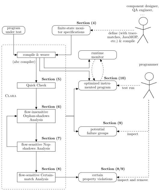
Figure 5 gives an overview of Clara. At the beginning of the work flow (top right) stands a component designer who wrote an application interface (API), which comes with usage requirements expressed as finite-state properties. In our running example, this would be the programmer who initially provides the “Connection” API. As part of the API, the designer specifies a runtime monitor which captures property violations at runtime, for instance as a tracematch. Further, the programmers uses a runtime-verification tool to automatically translate the high-level specification into an AspectJ aspect, annotated with a Dependency State Machine. We extended the tracematch implementation so that it automatically annotates the aspects that it generates. The authors of JavaMOP [Chen and Ro¸su 2007] are currently in the process of extending their tool accordingly, and many other runtime verification tools will likely support Dependency State Machines in the future.
The programmer invokesClarawith the aspect-based monitor definition and a program as inputs. Clara compiles the code of the runtime monitor and “weaves” the monitor into the program under test, i.e., instruments the program with code that notifies the monitor about state transitions that the program performs. (Clarauses the AspectBench Compiler [Avgustinov et al. 2005] for weaving.) Clara then invokes its static analysis engine, which may include third-party static analyses. These analyses collect information about the finite-state property to approximate the set of relevant instrumentation points. Whenever an analysis declares that an instrumentation point does not affect whether or not the program violates the property, Clara disables the instrumentation for this property at this point. The result is an optimized instrumented program that updates the runtime monitor only at program points at which instrumentation remains enabled.
Our Certain-match Analysis also reports certain matches to the programmer. Such matches denote program locations that certainly lead to a property violation if executed.
Claraoutputs a list ofpotential failure groups. Each group is a set of shadows containing a single potential point of failure, i.e. a shadow at which the program may violate the stated property at runtime, along with a set of context shadows, which trigger events on the same objects as the potential point of failure, and hence may contribute to the property violation. This presentation of our analysis results was particularly useful for manual inspection.
4. DEFINITIONS
We now provide a formal description of finite-state runtime monitors. These definitions allow us to reason formally about the correctness of our static analyses.
Clara
(abc compiler) compile & weave program under test finite-state moni-tor specifications Quick Check flow-insensitive Orphan-shadows Analysis flow-sensitive Nop-shadows Analysis flow-sensitive Certain-match Analysis optimized instru-mented program potential failure groups certain property violations programmer component designer, QA engineer, . . . runtime monitor Section (4) Section (5) Section (6) Section (7) Section (8) Section (8/9) Section (9) Section (10) test run inspect
inspect and remove define (with trace-matches, JavaMOP,
etc.) & compile
Fig. 5: Overview ofClara
4.1. Runtime Monitors
We begin by stating standard definitions from automata theory.
Definition1 (Finite-state machine). A non-deterministic finite-state machine M is a
tuple (Q,Σ, q0,∆, QF), whereQis a set of states, Σ is a set of input symbols,q0the initial state, ∆⊆Q×Σ×Qthe transition relation andQF ⊆Qthe set of accepting (final) states. We will also call final states “error states”. We consider that a finite-state property has been violated when the state machine associated with the property reaches a final state. (In that sense, our properties are negative properties which describe forbidden behaviour.)
Definition2 (Words, runs and acceptance). A word w = (a1, . . . , an) is an ele-ment of Σ∗; word w has length |w| = n. We define a run ρ of M on w to be a sequence (q0, qi1, . . . , qin) which respects the transition relation ∆; that is, ∀k ∈
[0, n). ∃ak. (qik, ak+1, qik+1) ∈ ∆, with i0 := 0. A run ρ is accepting if it finishes in an accepting state, i.e. qin ∈ QF. We say that M accepts w, and write w∈ L(M), if there
exists an accepting run ofMonw.
We further require the notion of a prefix.
Definition3 (Set of prefixes). Letw∈Σ∗ be a Σ-word. We define the setpref(w) as:
pref(w) :={p∈Σ∗| ∃s∈Σ∗ such thatw=ps}.
Definition4 (Matching prefixes of a word). Let w∈ Σ∗ be a Σ-word and L ⊆ Σ a
Σ-language. Then we define the matching prefixes of w (with respect to L) to be the set of prefixes ofwalso belonging toL:
matchesL(w) :=pref(w)∩ L.
We writematches(w) instead ofmatchesL(w) ifLis clear from the context.
Clarauses finite-state machines to model and implement runtime monitors.Clarafirst generates a finite-state machine from the provided monitor definition. It then instruments the program under test such that the program will issue a trace (effectively a word in Σ∗) when executed. The finite-state machine reads this trace as input. The instrumented program executes the monitor’s associated error handler whenever the machine reaches an accepting state, i.e., whenever the prefix of the trace read so far is an element of L.
Generalizing to multiple monitor instances.It would be a severe restriction to allow for
only one monitor instance at runtime. Consider ConnectionClosed from Section 1. Programs typically use many simultaneously-active connection objects, where each connection object could be in a different state. Modern runtime monitoring systems therefore allow the user to defineparametricruntime monitors [Chen and Ro¸su 2009]. A parametric monitor effectively comprises a set of monitors, one monitor for every variable binding. Clara’s semantics is defined over parametric monitors, which we now define.
Definition5 (Variable Binding). LetO be the set of all runtime heap objects andV a
set of variables appearing in monitor specifications. Then we define a variable bindingβ as a partial function β:V *O. We call the set of all possible variable bindingsB.
Due to variable bindings, runtime monitoring does not operate on a single trace from Σ∗, but rather on a parametrized trace, consisting of a trace of parametrized events. Parametrized events associate bindings with events.
Definition6 (Parametrized event). A parametrized event ˆe is a set of pairs (a, β) ∈
Σ× B. ˆΣ is the set of all parametrized events. A parametrized trace is a word from ˆΣ∗. We use sets of pairs because one program event can yield multiple monitoring events. This occurs when multiple monitors listen for the same program events.
Every monitored program will generate a parametrized event trace when it executes. The instrumentation thatClarainserts into the program notifies the runtime monitor at every event of interest about the monitor transition symbola∈Σ as well as the variable binding
β ∈ Bidentifying all monitor instances that need to process the event.
For instance, executing the program from Figure 4b with the ConnectionClosed monitor-ing aspect from Figure 2 yields the followmonitor-ing parametrized trace:
{(CLOSE, c7→o(c1))} {(WRITE, c7→o(c2))} Here, o(v) represents the object referred to by program variablev.
However, monitor instances are ordinary finite-state machines, which process symbols from the base alphabet Σ, rather than parametrized events from ˆΣ. We therefore project the unique parametrized program trace that the program generates onto a set of ground traces—words over Σ. Every ground trace is associated with a binding β and contains all events whose bindings are compatible withβ.
Definition7 (Compatible bindings). Let β1, β2 ∈ B be two variable bindings. These
bindings are compatible if they agree on the objects that they jointly bind: compatible(β1, β2) :=∀v∈(dom(β1)∩dom(β2)). β1(v) =β2(v).
Definition8 (Projected event). For every parametrized event ˆeand bindingβ we define
a projection of ˆewith respect toβ: ˆ
e↓β:={a∈Σ| ∃(a, βa)∈eˆsuch thatcompatible(βa, β)}.
Definition9 (Parametrized and projected event trace). Any finite program run induces
a parametrized event trace ˆt = eb1. . .cen ∈ ˆ
Σ∗. For any variable binding β we define a projected trace ˆt↓β ⊆ Σ∗ by only keeping events compatible with β. Formally, ˆt↓β is the smallest subset of Σ∗for which, ifef(i):=ebi↓βfor alli∈ {1, . . . , n}, withf : [1, n]→[1, m] order-preserving andm≤n, then
e1. . . em∈ˆt↓β.
In the following we will call traces liket, which are elements of Σ∗, ground traces, as opposed to parametrized traces, which are elements of ˆΣ∗.
In our semantics, a runtime monitor will execute its error handler whenever the prefix read so far of one of the ground traces of any variable binding is in the language described by the state machine. We exclude the empty trace (with no events) because this trace cannot possibly cause the handler to execute: empty traces contain no events, while we require handlers to see at least one event before executing. This yields the following definition.
Definition10 (Set of non-empty ground traces of a run). Let the trace ˆt ∈ Σˆ∗ be the
parametrized event trace of a program run. Then the set groundTraces(ˆt) of non-empty ground traces of ˆt is:
groundTraces(ˆt) := [ β∈B ˆ t↓β ∩Σ +.
We intersect with Σ+ to exclude the empty trace.
Definition11 (Matching semantics of a finite-state runtime monitor). Let M :=
(Q,Σ, q0,∆, QF) be a finite-state machine. Let ˆt ∈ Σˆ∗ be a parametrized event trace generated by a program execution. We say that ˆtviolates the property described by Mat positioniwhen:
∃t∈groundTraces(ˆt).∃p∈matchesL(M)(t).|p|=i.
By our definition of runtime monitoring, the monitor will execute its error handler at every position iat which ˆtviolates the monitored property.
Correct definitions of Dependency State Machines. In the future we expect runtime
verifi-cation tools that currently generate runtime monitors as AspectJ aspects to instead generate aspects annotated with Dependency State Machines. That way, the monitors become au-tomatically analyzable by Clara. The only requirement on Clara’s clients, i.e., on the runtime verification tools, is that the semantics of the generated Dependency State Machine
(as defined by Definition 11) must coincide with the semantics of the annotated monitor. Such proofs are simple to conduct for the two tools we tried, tracematches and JavaMOP, and we expect them to also be simple for other finite-state runtime monitoring tools.
4.2. Statically optimizing parametrized monitors
Our definition of the matching semantics for finite-state runtime monitors states when a runtime monitor needs to trigger on an input trace ˆt. Any sound static optimization of such runtime monitors must obey this semantics, i.e., must guarantee that the monitors trigger (or don’t trigger) exactly at the same times with or without the optimization.
We next define a runtime predicate called mustMonitor that, for every symbola ∈ Σ, every parametrized trace ˆt, and every position i ∈ Nin this trace, returns true when a -transitions must be monitored at positioniof ˆtaccording to the above semantics andfalse when the transition need not be monitored, i.e., when processing of the a-transition may safely be omitted.
mustMonitor: Σ×( ˆΣ)∗×N → B
mustMonitor(a,ˆt, i) :=∃t∈groundTraces(ˆt) such thatnecessaryTransition(a, t, i).
The mustMonitor predicate depends on the predicate necessaryTransition(a, t, i). This predicate is a free parameter to our semantics, enabling the use of any suitable definition ofnecessaryTransition. Our semantics demand thatnecessaryTransitionmust meet the fol-lowing soundness condition.
Condition1 (Soundness condition fornecessaryTransition). Any sound
implementa-tion ofnecessaryTransitionmust satisfy: ∀a∈Σ.∀t=a1. . . ai. . . an∈Σ+.∀i∈N.
a=ai∧matchesL(a1. . . an)6=matchesL(a1. . . ai−1ai+1. . . an) =⇒necessaryTransition(a, t, i).
In other words, a transitionamust be monitored at positioniwhenever not monitoringa
atiwould change the set of matches for a runtime monitor. Note that it is only possible to approximate necessaryTransition; the optimal function is uncomputable because it would require knowledge about future events: the most accurate possible necessaryTransition re-quires that, while observing thei-th event, one would need to know whether the remainder of the trace will or will not lead to further matches.
Sections 5 through 7 define three different approximations tonecessaryTransitionthat are computable at compile-time. We will prove that these approximations imply the soundness condition.
5. SYNTACTIC QUICK CHECK
The Quick Check is, as the name suggests, a simple analysis that can execute within millisec-onds. This analysis rules out transitions that have no effect because they are unreachable or have no effect in the program under analysis. The Quick Check only uses syntactic informa-tion which is available to the compiler after it inserts runtime monitoring instrumentainforma-tion; it runs in time polynomial in runtime monitor size and linear in program size.
Examples and Discussion
As an example, consider again the ConnectionClosed automaton from Figure 1 in combina-tion with a program that closes and perhaps reconnects conneccombina-tion objects but never writes to them (for instance, the program from Figure 4a without line 4). In this case, the Quick Check first removes all WRITE-transitions from the finite-state machine. Next, the
algo-rithm finds that all states have become unproductive.1This way, the Quick Check correctly determines that no symbol requires monitoring.
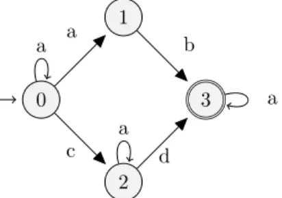
The Quick Check sometimes eliminates only some of the transitions in a finite-state machine. Consider the automaton in Figure 6. In this example, if the program can produce all events except b events, then the Quick Check will reduce the state machine to states 0,2, and 3. Along the remaining acyclic path through the automaton, the symbols c and
dchange the machine’s state, and hence require monitoring. The symbola, however, does not require monitoring: on the remaining productive states 0,2,and 3,a-transitions always loop. The Quick Check would report thatb must be monitored, but that is moot, since b
events cannot occur in our program.
Similarly, consider the case where the program can produce all events butdevents. The Quick Check would determine that symbolsa, bandcrequire monitoring:aandb because they transition from one productive state to another, andcbecause states 1 and 3 have no outgoing c-transition and therefore would possibly reject words when reading ac.
To clarify the last point, assume a program that generates a trace “a c b”. The monitor should not trigger on this trace because “a c b” is not in the language of this finite-state machine. But if we failed to monitorc, then the state machine would effectively only observe the partial trace “a b”. This trace would drive the finite-state machine into its final state, which would be incorrect. This point applies to our subsequent analyses as well.
The Quick Check generally works well in cases where properties do not apply to the program under test. For instance, in the ConnectionClosed example, the Quick Check would succeed only if the program either never closes connections or never writes to them. One may wonder why monitors would track properties which a program can obviously never violate. We envision a scenario in which monitors and programs are written by different people. In our example, the monitor for the ConnectionClosed property would be written by the developers of the Connection interface, and distributed along with that interface. The library developers cannot know in advance which parts of the distributed properties actual programs will use.
Algorithm
Algorithm 1 computes a set of symbols that need monitoring, given a set L of labels that occur. First, the set ∆Lfilters out transitions from the monitor carrying labels that do not occur in the program. Next, the setQpretains only productive states fromQ—states that are reachable through ∆L from the initial state q0 and which can reach some final state in QF. The set of productive transitions ∆p then retains from ∆L only those transitions that lead from and to productive states. Finally, the algorithm returns the set of symbols either appearing in non-looping productive transitions or for which a productive state has 1A productive state is a state that is reachable from an initial state and from which some final state can
be reached. 0 1 2 3 a b c d a a a
no outgoing transition at all. The latter class of symbols must remain, as they cause input words to be rejected.
Algorithm 1 Compute symbols required under Quick Check. Input: set Lof labels of all transition statements in the program Output: setsymbolsThatNeedMonitoring
1: let∆L={(qs, a, qt)∈∆|a∈L} in
2: letQp={q∈Q| ∃path in ∆L from q0 toq ∧ ∃path in ∆L from qtoqf ∈QF}in
3: let∆p={(qs, a, qt)∈∆L|qs∈Qp∧qt∈Qp}in
4: return {a∈Σ| ∃qs∈Qp.((∃qt∈Qp.(qs, a, qt)∈∆p∧qs6=qt)∨ (¬∃qt∈Qp.(qs, a, qt)∈∆p))}
To connect the Quick Check to Clara’s optimization engine, we simply define a new predicatenecessaryTransitionQCas an instantiation of the predicatenecessaryTransition:
necessaryTransitionQC(a, t, i) :=a∈symbolsThatNeedMonitoring. Soundness of the Quick Check
To show that the Quick Check meets the soundness condition from Section 4 we need to show the following:
∀a∈Σ ∀t=a1. . . ai. . . an ∈Σ+ ∀i∈N:
a=ai∧matchesL(a1. . . an)6=matchesL(a1. . . ai−1ai+1. . . an) =⇒necessaryTransitionQC(a, t, i)
Proof. Follows immediately from Algorithm 1. Assume matchesL(a1. . . an) 6= matchesL(a1. . . ai−1ai+1. . . an). Because the matchessets differ, we know that after hav-ing read the prefix a1. . . ai−1, the automaton must either move from one productive state to another (ensured by the first disjunct of the return value and the definition of ∆p) or it must move to no state at all (ensured by the second disjunct). In either case,
a∈symbolsThatNeedMonitoring, sonecessaryTransitionQC(a, t, i) holds.
6. FLOW-INSENSITIVE ORPHAN-SHADOWS ANALYSIS
The flow-insensitive Orphan-shadows Analysis sharpens the results of the Quick Check by taking pointer information into account: it removes transitions which are ineffective because they are bound to objects that never match. The Orphan-shadows Analysis runs in time polynomial in runtime monitor size and in shadow count; it incurs setup overhead beyond the Quick Check, though, because it relies on points-to information. In particular, the Orphan-shadows Analysis models runtime objects using the static abstraction of points-to sets. For any program variable p, the points-to set pointsTo(p) is the set of all allocation sites, as represented by newstatements, that can reachpthrough a chain of assignments.
Example and Motivation
Recall the example from Figure 4b, which never matched because the CLOSE and WRITE events occurred on different objects: the points-to set for variable c1referenced at line 4 would contain thenewstatement at line 2, while the points-to set for variablec2referenced at line 5 would contain the newstatement at line 3. The points-to sets pointsTo(c1) and pointsTo(c2) would be disjoint: it is impossible forc1andc2to point to the same object. At runtime, variable bindingsβconnect monitor variables to runtime heap objects. Points-to sets can serve in the place of these heap objects, and we denote static variable bindings which use points-to sets by ˜β. Static variable bindings summarize runtime bindings. That is,
letv be a monitor specification variable andobe a runtime object. Thenβ(v) =oimplies that owas created at one of thenewstatementsnsuch thatn∈β˜(v).
Bindings are critical to matching. A runtime monitor only reaches its error state after having processed appropriate transitions with a “compatible variable binding”. That is, each pair of transitions comes with bindings βi and βj; we require that, for each pair of transitions leading to a match,compatible(βi, βj).
We statically approximate variable bindings using points-to sets. To do so, we define a static approximation stCompatible of the compatibility predicate compatible. Instead of requiring equality as in the runtime case, we instead declare two bindings to be statically compatible when their points-to sets overlap on their joint domains. That is, variables in common may possibly be assigned the same objects at runtime:
stCompatible( ˜β1,β˜2) :=∀v∈(dom( ˜β1)∩dom( ˜β2)).β˜1(v)∩β˜2(v)6=∅.
Shadows.Programs containshadows, which are static program points causing finite-state
machine transitions. Pointcuts in the declaration of the dependency state machine induce shadows. Each shadow binds some number of variables. At runtime, shadows cause events, and their variables become bound to heap objects. We use points-to sets to approximate the heap objects occurring in variable bindings. We denote the set of all shadows by S.
We say that two shadows s1 and s2 are compatible, and write stCompatible(s1, s2), if their bindings are statically compatible. Like most points-to analysis clients, our static analysis exploits the negation ofstCompatible: it disregards transitions or events that can, in combination, only lead to incompatible variable bindings. Such events clearly cannot drive the runtime monitor into an error state.
Algorithm
Algorithm 2 presents the algorithm for the Orphan-shadows Analysis. This algorithm runs the Quick Check once for each shadow s. Each invocation of the Quick Check is told that only the labels for shadows compatible withsexist. Thensis necessary for Orphan-shadows Analysis iff, considering only the set of shadows compatible withs, the Quick Check declares that sis necessary.
To connect the Orphan-shadows Analysis to Clara’s optimization engine, we proceed analogously to the Quick Check, and define the predicate necessaryTransitionOSA, as a second instantiation ofnecessaryTransition:
necessaryTransitionOSA(a, t, i) :=shadow(ai)∈necessaryShadows
6.1. Soundness of the Orphan-shadows Analysis
To show soundness for the Orphan-shadows Analysis (as per Section 4) we must show: ∀a∈Σ ∀t=a1. . . ai. . . an∈Σ+ ∀i∈N:
a=ai∧matchesL(a1. . . an)6=matchesL(a1. . . ai−1ai+1. . . an) =⇒necessaryTransitionOSA(a, t, i)
Proof. Assume matchesL(a1. . . an) 6= matchesL(a1. . . ai−1ai+1. . . an). As with the Quick Check, after having read the prefixa1. . . ai−1, the automaton must either move from one productive state to another or it must move to no state at all (because no current state has aai-transition). In either case, the disequality implies that the transition at position i Algorithm 2 Compute symbols required under Orphan-shadows Analysis
Output: set necessaryShadows
1: functioncompSyms(s) ={l∈L| ∃s0∈ S.stCompatible(s, s0)∧l=label(s0)}
must have a variable binding compatible with all bindings of all transitions at positions 1 through n. Therefore, by construction, it must hold that shadow(ai)∈ necessaryShadows and hencenecessaryTransitionOSA(a, t, i).
6.2. Benefits of a demand-driven pointer analysis
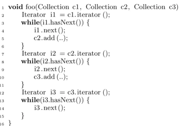
To compute points-to sets we use the demand-driven, refinement-based, context-sensitive, flow-insensitive pointer-analysis by Sridharan and Bod´ık [2006]. Context-sensitive analyses distinguish objects that are allocated in different calling contexts but using the same alloca-tion sites, e.g., multiple iterators that are all instantiated by calling the same iterator()
method in the Java runtime library. Sridharan and Bod´ık’s analysis starts with context-insensitive information computed by Spark [Lhot´ak and Hendren 2003] and then refines the context-insensitive results with additional context information on demand. This is relatively fast because the refinement only needs to be computed for variables that we are interested in, i.e., for program variables that the monitor actually refers to. The pointer analysis is also demand-driven: it computes context information up to a certain level, defined by a user-provided quota. If the refined information is precise enough to distinguish the computed points-to sets from others, then we are done. Otherwise, we can opt to have the points-to set refined further with a higher quota.
To use the demand-driven approach, we augmented points-to sets with wrappers. Upon an emptiness-of-intersection query for points-to setspointsTo(c1) andpointsTo(c2), the wrap-pers compute a first approximation ofpointsTo(c1) andpointsTo(c2). If this approximation is sufficient to determine thatpointsTo(c1)∩pointsTo(c2) =∅, then the wrappers immedi-ately returnfalse. Otherwise, the wrappers refine the approximations of both points-to sets and re-iterate until finding two approximations with empty intersection (yieldingfalse), or until exhausting a pre-defined quota, yielding true.
7. FLOW-SENSITIVE NOP-SHADOWS ANALYSIS
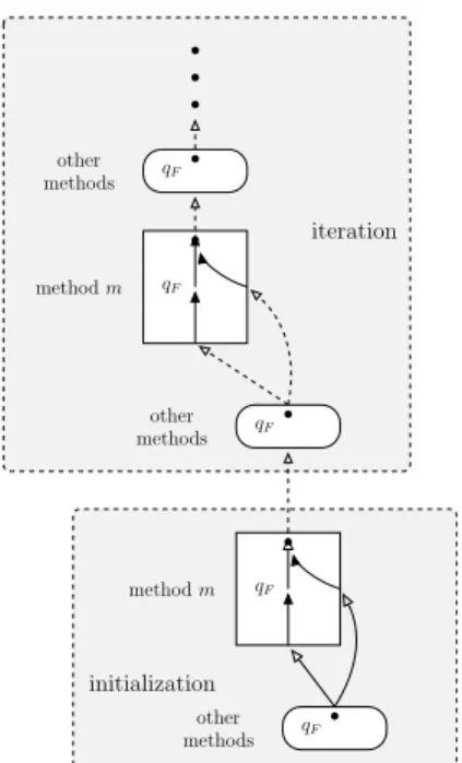
The key technical contribution in this work is our novel Nop-shadows Analysis. This analysis is a flow-sensitive intra-procedural analysis, which incorporates inter-procedural information from the flow-insensitive Orphan-shadows Analysis. Its abstractions track, for each program statement, (1) the set of heap objects that could be in each state of the Dependency State Machine, and (2) sets of states from which objects could reach a final state. Using this information, our analysis identifies nop shadows, which are shadows that do not affect whether the Dependency State Machine can reach a final state.
Two main reasons motivated our design decision to use an intra-procedural analysis. First, intra-procedural analyses almost always run more quickly than inter-procedural analyses, since they consider far less code. Our second reason is empirical. We manually investi-gated the still-active instrumentation points in our benchmarks following the application of the flow-insensitive Orphan-shadows Analysis, and found that, in most cases, intra-procedural analysis information suffices to rule out unnecessary instrumentation points, when combined with coarse-grained inter-procedural summary information available from the Orphan-shadows Analysis. Most procedures appear to locally establish the conditions that they require to satisfy the type of conditions that we currently specify and verify with Clara. The results presented in this paper confirm these findings.
We next explain the need for flow-sensitivity by presenting some code which exercises our running example, the ConnectionClosed tracematch. Our first example is straight-line code involving a single connection object; however, in Section 7.6, we discuss how our analysis handles loops, multiple methods, and events on arbitrary combinations of aliased objects.
7.1. Example
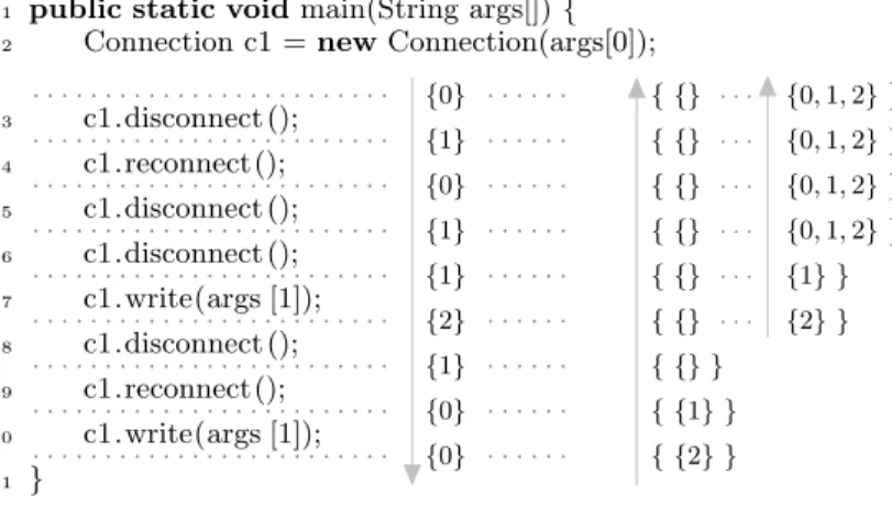
Figure 7 presents example code. It is annotated with a simplified version of the analysis information that our analyses will compute; an explanation of this information follows.
The code creates a connection and executes some operations on that connection, all of which cause transitions on the ConnectionClosed aspect. Because our example code only manipulates one connection object, we can defer our discussion of aliasing to Section 7.6.1. While this example is contrived, it demonstrates the possibilities for optimization by taking control flow into account. (The flow-insensitive Orphan-shadows Analysis does not suffice: both disconnect and reconnect events occur on the same object.) The only events that must be monitored to trigger the monitor for this example at the right time are 1) the write at line 7 and 2) one of the two disconnect events at lines 5 and 6. In particular, the disconnect and reconnect operations at lines 3 and 4 do not need to be monitored: they are on the prefix of a match, but the match can be completed without monitoring this prefix. Conversely, the operations at lines 8 to 10 do not lead to a pattern violation and hence need no monitoring either. Soundness requires monitoring at least one of the two disconnects at lines 5 and 6, but not both.
Using the Nop-shadows Analysis results, the compiler need only retain instrumentation at lines 5 and 7, or 6 and 7—the minimal set of instrumentation points guaranteeing an optimized instrumented program will report an error if and only if the un-optimized program would have reported an error.
7.2. Analysis Overview
The Nop-shadows Analysis identifies nop shadows one at a time, by combining results from two analysis phases. The first phase uses a backward dataflow analysis to tell apart, for every statement in a method, (1) states which may possibly lead (in the rest of the program) to a final state (“hot states”) and (2) states that will never give rise to a final state (“cold states”). The second phase uses a forward dataflow analysis to compute possible monitor states at each statements. The analysis can then identify nop shadows by combining results from the two phases.
Let shadows lead fromq toq0. Thensmust be monitored, i.e., is not a nop shadow, if there is some continuation for which q andq0 are not in the same equivalence class. Two situations require shadows to remain enabled: (1) a transition atsmay move the automaton from a hot to a cold state, leading to false positives if disabled; or (2) a transition from a cold state to a hot state, leading to false negatives if disabled. In (1), disablingsmay lead to false positives at runtime; because the transition is disabled, the monitor state remains hot and the monitor may therefore signal a violation that swould have prevented. In (2),
1 public static voidmain(String args[]){ 2 Connection c1 =newConnection(args[0]); 3 c1.disconnect (); · · · {0} · · · { {} · · · {0,1,2} } 4 c1.reconnect (); · · · {1} · · · { {} · · · {0,1,2} } 5 c1.disconnect (); · · · {0} · · · { {} · · · {0,1,2} } 6 c1.disconnect (); · · · {1} · · · { {} · · · {0,1,2} } 7 c1.write(args [1]); · · · {1} · · · { {} · · · {1} } 8 c1.disconnect (); · · · {2} · · · { {} · · · {2} } 9 c1.reconnect (); · · · {1} · · · { {} } 10 c1.write(args [1]); · · · {0} · · · { {1} } 11 } · · · {0} · · · { {2} }
the transition moves the automaton from cold to hot. In this case, disabling smay yield a false negative; the monitor could fail to signal an actual violation.
We can disablesin all other cases: if, for all continuations ofs, all possible source states
q and target states q0 are either all hot or all cold. Such a transition would not change whether or not the automaton matches, and we declare thatsis a nop shadow.
Dependencies between shadows require us to iterate our algorithm until it reaches a fixed point, removing one shadow at a time.
We describe the algorithm by first discussing the forward and backward phases, as they apply to a single set of variable bindings; Section 7.6.1 presents our full abstraction, which maps Dependency State Machine states to logical formulas over binding representatives.
7.3. Forward pass
The forward pass determines, for each statement s, the set of automaton states that the automaton could be in at statements. The forward analysis works on a determinized input state machine2.
Clarabuilds the deterministic automaton using subset-construction:
Definition12 (Determinizing a non-deterministic state machine). LetL ⊆Σ∗be a
reg-ular Σ-language and let M = (Q,Σ,∆, Q0, F) be a non-deterministic finite-state ma-chine with L(M) = L. Then we define the deterministic finite-state machine det(M) as det(M) := (P(Q),Σ, δ, Q0,Fˆ) by:
δ = λQs.λa.{qt∈Q| ∃qs∈Qs such that∃(qs, a, qt)∈∆}; ˆ
F = {QF ∈ P(Q)| ∃q∈QF such thatq∈F}.
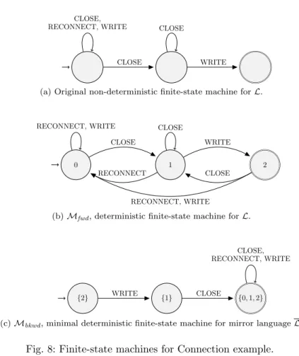
Figure 8a reproduces the non-deterministic finite-state machine for the ConnectionClosed example. Figure 8b shows the equivalent deterministic finite-state machine. We have as-signed a fresh state number to each state in the deterministic automaton.
In Figure 7, next to the downwards-pointing arrow, we have annotated each statement with the states of the deterministic automaton just before and after executing that state-ment. In this example, the program has only a single control-flow path, and therefore our analysis will only associate a single state with each statement. However, if there are mul-tiple control-flow paths reaching a statements, and the execution along these paths yields different states q1 and q2, then our analysis will associate bothq1 and q2 with s—it does not merge states. In the sequel, we will denote the set of source states associated withsby sources(s). Also, we will refer to the deterministic finite-state machinedet(M) asMfwd. 7.4. Backward pass
The backward analysis determines, for every statement s, sets of states that are “hot” at
s; it finds one set for every possible continuation of the control flow afters which reaches the final state. Like the forward analysis, the backward analysis uses a determinized state machine. In particular, it uses a determinized state machine for the mirror language L, which consists of the reverse of every word in L. Given a non-deterministic finite-state machineMwithL(M) =L, one can easily obtain a non-deterministic finite-state machine rev(M) acceptingLby reversing the transition function.
For any non-deterministic finite-state machine M, L(rev(M)) =L(M).
Our backward analysis operates on the state machine Mbkwd:=det(rev(Mfwd)).
2Determinizing ensures that the state machine will be in only one state at a time. This simplifies the
CLOSE CLOSE,
RECONNECT, WRITE
WRITE CLOSE
(a) Original non-deterministic finite-state machine forL.
0 1 2 CLOSE RECONNECT, WRITE WRITE CLOSE RECONNECT CLOSE RECONNECT, WRITE
(b)Mfwd, deterministic finite-state machine forL.
{2} WRITE {1} CLOSE {0,1,2}
CLOSE, RECONNECT, WRITE
(c)Mbkwd, minimal deterministic finite-state machine for mirror languageL. Fig. 8: Finite-state machines for Connection example.
Note that L(Mbkwd) =L. Figure 8c shows the state machine that the backward analysis uses for the ConnectionClosed example. The states of Mbkwd are actually subsets of the state set of Mfwd; we labelled every state of Mbkwd with the corresponding state set of det(rev(M)) (Figure 8b). For presentation purposes, we omitted the reject state from the Figure; the reject state represents the empty state set. By construction,Mbkwdis minimal. (See [Brzozowski 1962] for a proof.)
The forward analysis conceptually starts at the beginning of the program execution. (Since our analyses are intra-procedural, we use Orphan-shadows Analysis to summarize caller effects). The backward analysis, on the other hand, starts at every statement which potentially reaches a final state, i.e., at every shadow s such that label(s) = l with an
l-transition into a final stateqF ∈F.
In Figure 7, we show how the states of Mbkwd evolve through the backward analysis. At first, the only label that can bring the ConnectionClosed monitor into a final state is a WRITE. The analysis therefore starts immediately before every write statement. The analysis then proceeds exactly as the forward analysis. For instance, starting in state {2} and reading a WRITE through the automaton in Figure 8c, the analysis infers that the next state, just before the WRITE, is{1}. Due to the symmetries between the analyses, we have implemented the forward and backward analyses using a common code base; the only difference is in the inputs (state machines, control-flow graphs) that we provide to them.
7.5. Determining Nop shadows
The analysis information in Figure 7 enables us to identify and disable nop shadows. Our notion of a nop shadow is related to the novel idea of continuation-equivalent states. We say that states q1 and q2 are continuation-equivalent at a shadow s, or simply equivalent at s, and write q1 ≡s q2, if, for all possible continuations of the control flow after s, the dependency state machine reaches its final state at the same program points, whether we are in stateq1 orq2at s. We formally define this equivalence relation as follows.
For every shadow s, call the sets of states computed by the backward analysis imme-diately after s the futures ofs. Further, call the states computed by the forward analysis immediately before s the sourcesof s, and for every state q in sources(s), let target(q, s) be the target state reached after executing an s-transition from q. For instance, for the disconnect statement at line 5 of Figure 7 we have:
futures(line 5) = { {},{0,1,2} }; sources(line 5) = {0};
target(0,line 5) = 1.
We further define continuation-equivalence for states as:
q1≡sq2 := ∀Q∈futures(s). q1∈Q⇔q2∈Q.
A shadow is a nop shadow when it transitions between states in the same equivalence class, unless the target state is an accepting state. (Because reaching a final state triggers the monitor, such transitions have an effect even though they switch between equivalent states.) Recall thatF is the set of accepting, i.e., property-violating, states ofMfwd.
Definition 13. A shadow at a statementsis anop shadow if:
∀q∈sources(s). q≡starget(q, s)∧target(q, s)6∈F.
The first conjunct states a nop-shadow transitions only between states that are in the same equivalence class. However, if target(q, s) ∈ F, then the shadow triggers the run-time monitor. According toClara’s monitoring semantics, a monitor must signal repeated property violations every time the violation occurs—some monitors execute error-handling code. For instance, on “c . disconnect (); c . write (); c . write()”, the monitor should signal a violation after both WRITE events. However, the second WRITE event does not change the monitor’s state; we have 2 =target(2, s) = 2, so we must explicitly handle such cases.
Examples. The disconnect statement at line 5 of Figure 7 has source(s) = {0} and
target(0, s) = 1. For both sets Qfut ∈ futures(s) ={ {},{0,1,2} }, 0 ∈ Qfut ⇔1 ∈ Qfut. Consequently, we have 0≡s1. Because 16∈F, sis a nop shadow.
The write statement at line 7 is different. Here,source(s) ={1}andtarget(1, s) = 2. The set Qfut ={2} ∈futures(s) has 2 ∈Qfut but 16∈Qfut. Hence, 16≡s 2, i.e.,s is not a nop shadow, and must therefore remain enabled.
Remark on minimization.Although any machine accepting the mirror language would
work for the backward analysis, the definition of nop shadows explains why we use a mini-mal deterministic finite-state machine: in a minimini-mal state machine, all (forward-)equivalent states are collapsed together. The collapsed state will be labeled with a larger set Qfut of Mfwd states than the un-collapsed sets would have been. Hence, after collapsing equivalent states, more sets Qfut will contain both source and target states.
Need to re-iterate. Our example program contains several nop shadows. For instance, all
shadows in lines 3–6 from Figure 7 are nop shadows, and indeed it is sound to disable any single shadow from that set. However, we can only remove shadows one-by-one: after dis-abling a shadow, we need to re-compute the analysis information for its containing method,
because disabling a shadow changes the monitor’s transition structure within the method. For instance, in our example, disabling both CLOSE transitions at lines 5 and 6 is unsound: removing both shadows leads to the monitor not reaching its final state at line 7.
Algorithm 3 presents the main loop of the Nop-shadows Analysis. For each shadow-bearing method in the program, this algorithm iterates the forward and backwards passes, along with the Orphan-shadows Analysis (when necessary), greedily removing shadows until it reaches a fixed point. On our benchmarks, two iterations of the outer loop always sufficed. Algorithm 3 Main loop for Nop-shadows Analysis.
repeat
foreach methodm still bearing enabled shadowsdo repeat
compute forward and backward analysis results form. if mcontains nop shadows then
arbitrarily choose and remove any one nop shadow. re-run Orphan-shadows Analysis on shadows from m. end if
untilno nop shadows remain inm.
if we have removed any nop shadows frommthen re-run Orphan-shadows Analysis on entire program. end if
end for
untilwe failed to remove a nop shadow in the previous iteration
In the example, the algorithm would leave one of the shadows at lines 5–6, and the shadow at line 7—exactly the minimal set of shadows in this case.
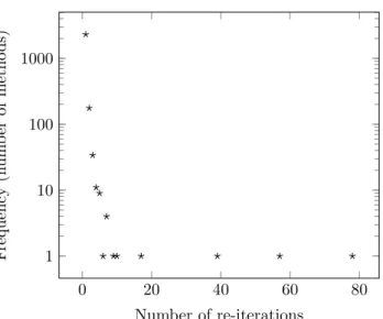
Figure 9 shows how often we re-iterate the analysis of each method, summarizing results over all methods from our benchmark set where Nop-shadows Analysis applies. Observe that we iterate only a few times for the vast majority of cases—this number is bounded by the number of still-enabled shadows in the method—and there are only twelve cases in which we have to iterate more than ten times. There was one method which required 78 re-iterations:fillArrayin classCompactArrayInitializerof the bloat benchmark with the FailSafeIter tracematch. This method contains a large number of statements that modify a collection (an instruction stream).
Our simplified discussion ignored the following features of Java code: (1) conditional control flow and loops,
(2) multiple methods with virtual dispatch, (3) aliased objects, and
(4) more general specification patterns referring to more than one object.
In the following, we explain an analysis that takes all of the above into account. We show that it is sound for any single-threaded Java program without reflection; in continuing work, we are investigating the use of dynamic information for circumscribing the potential impact of reflection on program behaviour [Bodden et al. 2011].
7.6. Full description of the Nop-shadows Analysis
We next present a sound implementation of the functionnecessaryTransition for the Nop-shadows Analysis. First, we motivate the need for flow-sensitive alias information. Recall that we defined the semantics of a dependency state machine over ground traces, which are projections of the single trace of parameterized events occurring at runtime. Our static
0 20 40 60 80 1 10 100 1000 Number of re-iterations F requency (n um b er of metho d s)
Fig. 9: Number of re-iterations per method (log scale).
analysis needs an analogue of projection to extract sub-traces for different variable bindings. We next define object representatives and explain how they are used in our abstraction.
7.6.1. Abstractions: object and binding representatives. Runtime monitors associate automaton states with variable bindings, i.e., mappings from free variables declared in the depen-dency state machine to concrete runtime objects. Because concrete runtime objects are not available at compile time, we use a static abstraction. We model a runtime binding
x = o(v1)∧y = o(v2) with a binding x = r(v1)∧y = r(v2), where r(vi) is the “ob-ject representative” ofo(vi). Object representatives are a static abstraction that uniformly incorporate aliasing information from multiple alias analyses. A full description of object representatives is beyond the scope of this paper; see [Bodden et al. 2008b] for details. In brief, object representatives almost transparently substitute for runtime objects by support-ing both may-alias and must-alias queries. The must-alias relation is the equality relation for object representatives. That is, when our implementation generates a set of two object representatives{r1, r2}, then ifr1andr2must-alias, we haver1=r2, so the set reduces to {r1}={r2}. This smaller representation saves time and memory during analysis.
At compile time, we implement object representatives as objects that are instantiated with a local variablevand statement sas parameter. An object representative hence represents the object pointed to by v at s. We omit s when it is clear from the context, or when
v has a single assignment, and write o(v). (Note that storing s is necessary because our internal representation is not in Static Single Assignment Form [Cytron et al. 1991]. If it were, scould be inferred from v.) Each object representativer1 also has access to a insensitive context-sensitive whole-program pointer analysis and to intra-procedural flow-sensitive must- and must-not-alias analyses, allowing the representative to decide aliasing relations to other object representativesr2on a best-effort basis (while defaulting to “may alias”, denoted r1≈r2). Table I summarizes the relations between object representatives.
We call the set of all object representatives ˜O. For any subset R⊆O˜ of object represen-tatives, we define setsmustAliases(R) andmustNotAliases(R) as follows:
mustAliases(R) := {r0 ∈O | ∃˜ r∈R such thatr=r0}; mustNotAliases(R) := {r0 ∈O | ∃˜ r∈R such thatr6=r0}.