arXiv:1803.00952v1 [math.OC] 2 Mar 2018
Miten Mistry1 Dimitrios Letsios1 Ruth Misener1 Gerhard Krennrich2 Robert M. Lee2
Abstract
Decision trees effectively represent the sparse, high dimensional and noisy nature of chemi-cal data from experiments. Having learned a function from this data, we may want to there-after optimize the function, e.g., picking the best chemical process catalyst. In this way, we may repurpose legacy predictive models. This work studies a large-scale, industrially-relevant mixed-integer quadratic optimization problem involving: (i) gradient-boosted ptrained re-gression trees modeling catalyst behavior, (ii) penalty functions mitigating risk, and (iii) penal-ties enforcing composition constraints. We de-velop heuristic methods and an exact, branch-and-bound algorithm leveraging structural prop-erties of gradient-boosted trees and penalty func-tions. We numerically test our methods on an industrial instance.
1. Introduction
Machine learning traditionally focusses on model predic-tivity and the computational expense of training. Opti-mization in the machine learning literature usually refers to the training procedure, e.g., model accuracy maximiza-tion (Sra et al.,2012;Snoek et al.,2012). Here, we inves-tigate optimization problems where the pretrained model prediction appears in the objective function. Modeling of physical and chemical processes is a major industrial exam-ple, where not only we require tools to predict the outcome of certain operating conditions, but also guidance towards a better set of operating conditions with respect to some performance criteria.
One option is using smooth and continuous machine learn-ing models, e.g., neural networks and support vector ma-chines with radial basis function kernels, to represent these physical and chemical processes. The resulting
optimiza-*
Equal contribution 1Department of Computing, Imperial Col-lege London, South Kensington, SW7 2AZ, UK2BASF SE, Lud-wigshafen am Rhein, Germany. Correspondence to: Miten Mistry <[email protected]>.
tion models may be addressed using local nonlinear opti-mization methods (Nocedal & Wright,2006). But feasible solutions come without a quantifiable guarantee of global-ity, even when using multi-start algorithms to escape local minima. The value of global optimization is known in the chemical processing literature (Boukouvala et al., 2016), e.g., local minima can lead to infeasible parameter estima-tion (Singer et al., 2006) or misinterpreted chemical data (Bollas et al.,2009). For applications where global opti-mization is less relevant, we still wish to develop optimiza-tion methods for discrete and non-smooth machine learning models, e.g., regression trees. Discrete optimization meth-ods allow repurposing a legacy model, originally built for prediction, into an optimization framework.
Also, although many machine learning techniques deal with feature correlation in training data, careful formula-tion of the subsequent optimizaformula-tion problem is essential to avoid implicit and unintentional feature causal roles. Con-sider, for instance, using historical data from a manufactur-ing process for quality maximization. The data may exhibit correlation between two process parameters: the tempera-ture and the concentration of a chemical additive. A ma-chine learning model of the system assigns weights to the parameters for future predictions. Lacking additional in-formation, numerical optimization may produce candidate solutions with temperature and concentration combinations that are drastically different from past observations. For instance, the machine learning model may incorrectly as-sociate temperature as responsible for an observed effect. A remedy to control the optimizer’s adventurousness is to include a term penalizing deviation from the training data subspace. Large values of this risk control parameter gen-erates conservative solutions. Smaller values of the penalty term explores regions with greater possible rewards at the cost of additional uncertainty.
This work elaborates on optimization methods for prob-lems whose objective includes gradient-boosted tree (GBT) model predictions (Friedman, 2001; Hastie et al., 2009) and risk terms to penalize deviation from the covariance structure of training data. Advantages of GBTs are myriad and justify their prominence among the winners in machine learning competitions (Chen & Guestrin, 2016; Ke et al., 2017). GBTs are robust to scale differences in the training data features, handle easily both categorical and
numeri-cal variables, and can minimize arbitrary differentiable loss functions. In addition, much work has been done to accel-erate the training of GBTs using graphical processing units and distributed computing resources (Zhang et al.,2017). Our approach formulates a mixed-integer quadratic pro-gramming (MIQP) problem whose objective consists of a discrete GBT trained function and a continuous convex penalty function. Our goal is to design exact optimization methods computing either globally optimal solutions, or solutions within a quantified distance from the global op-timum. We formulate the problem as an MIQP and solve a large industrial instance using commercial approaches. Mo-tivated by weak numerical findings, we develop a novel branch-and-bound method that exploits the tree ensemble combinatorial structure and the penalty function convexity in an integrated setting. Numerical analysis substantiates the strength of our approach.
The paper proceeds as follows. Section2formally defines the optimization problem. Section3 formulates the prob-lem as an MIQP and performs worst cases analysis. Sec-tion4 develops heuristics. Section5presents our branch-and-bound method. Section6presents a numerical analy-sis on a large-scale industrial instance. Finally, Section 7 concludes.
2. Optimization Problem
We analyze an optimization problem that consists of penalty functions and gradient-boosted tree (GBT) trained functions (Friedman, 2001; 2002). GBTs are a subclass of boosting methods (Freund, 1995). Boosting methods convert a collection of weak learners into a strong learner, where a weak learner is at least better than random guess-ing. For GBTs, the weak learners are classification and regression trees (Breiman et al.,1984).
In this work, our analysis is restricted to GBTs that only consist of regression trees, i.e., no categorical variables. Each level of a GBT splits variable xi into xi < v and xi ≥ v wherev is some constant defined at training. A GBT trained function is a collection of binary trees, each of which provides its own independent contribution when evaluating at x. The overall output is the sum of all tree evaluations. For a givenx, a tree evaluation follows a root-to-leaf path by queryingxi < vorxi ≥ vand following the left or right child, respectively, in each tree level. The leaf that corresponds toxcontains the tree’s contribution. Assume that we want to optimize a GBT trained function. Since the GBT function approximates an unknown func-tion, we may trust an optimal solution close to regions with many training points. To better approximate the remaining regions, we add a convex penalty term whose parameters are obtained by principal component analysis (PCA) on the
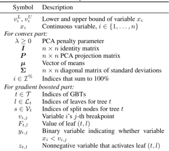
Table 1. Model sets, parameters and variables. Symbol Description
vLi,viU Lower and upper bound of variablexi
xi Continuous variable,i∈ {1, . . . , n}
For convex part:
λ≥0 PCA penalty parameter
I n×nidentity matrix
P n×nPCA projection matrix
µ Vector of means
Σ n×ndiagonal matrix of standard deviations i∈ I% Indices that sum to 100%
For gradient boosted part:
t∈ T Indices of GBTs
l∈ Lt Indices of leaves for treet s∈ Vt Indices of split nodes for treet
vi,j Variablei’sj-th breakpoint
Ft,l Value of leaf(t, l)
yi,j Binary variable indicating whether variable
xi< vi,j
zt,l Nonnegative variable that activates leaf(t, l)
training data. We consider the following optimization prob-lem: min vL≤x≤vU cvxλ(x) | {z } Convex Part + GBT(x) | {z } GBT Part , (1) cvxλ(x) =λ(I−P)Σ −1( x−µ) 2 2+ 100− X i∈I% xi 2 ,
andx = (x1, . . . , xn)⊤ is the variable vector. GBT(x) is the GBT trained function value atx. Penalty parameter λ ∈ R≥0, identity matrix I ∈ Rn×n, projection matrix P ∈ Rn×n, meanµ ∈ Rn, and diagonal matrix of stan-dard deviationsΣ∈Rn×ndefine the convex penalty term. Variable subsetI%⊆ {1, . . . , n}contains variablesx
ithat should sum close to 100%. ParametersvL,vU ∈ Rn en-force box constraints that lower and upper bound variable
x. Table1defines the model sets, parameters and variables. The additional term, which encourages the subsetI% ⊆ {1, . . . , n}of variablesxito sum close to 100%, is an arti-fact of the chemical processing application. We expect that the mass fraction of chemical compositions sums to 100 and, in the application, this term in the objective is equiva-lent to a constraint as there are several inert chemicals, i.e., variablesxithat participate in the mass fraction sum but do not appear in the GBTs. But, more generally, our method can include any convex penalty term.
The problem instances that this paper addresses consist of a sum of independently trained GBT functions. However, without loss of generality, we equivalently optimize a sin-gle GBT function which is the union of all original GBTs.
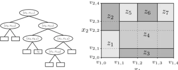
(x1, v1,1) (x2, v2,3) (x1, v1,3) z7 (x1, v1,2) z6 z5 (x2, v2,1) z4 z3 (x2, v2,2) z2 z1 v1,0 v1,1 v1,2 v1,3 v1,4 v2,0 v2,1 v2,2 v2,3 v2,4 z1 z2 z3 z4 z5 z6 z7 x1 x2
Figure 1. Gradient boosted tree trained in two dimensions. Left: gradient boosted tree. Right: domain partition.
3. Mixed-Integer Quadratic Formulation
Equation (1) consists of a continuous penalty function and a discrete GBT function. The discrete nature of the GBT function arises from the left/right decisions at the split nodes. So we consider a mixed-integer quadratic pro-gramming (MIQP) formulation. The main ingredient of the MIQP model is a mixed-integer linear programming (MILP) formulation of the GBT part which merges with the convex part via a linking constraint. The high level MIQP is:min
vL≤x≤vU
cvxλ(x) + [GBT MILP objective] (2a) s.t. [GBT MILP constraints], (2b)
[Variable linking constraints]. (2c) MILP approaches for machine learning show com-petitive performance for some important applications (Bertsimas & Mazumder, 2014; Bertsimas & King, 2016; Bertsimas et al., 2016; Bertsimas & Dunn, 2017; Miyashiro & Takano, 2015). The performance of MILP methods arises from the significant improvement of mixed-integer algorithms (Bixby, 2012) and the availability of commercial codebases.
3.1. GBT MILP Formulation
We form the GBT MILP using theMiˇsi´c(2017) approach. Figure1shows how a GBT partitions the domain[vL,vU] ofx. Optimizing a GBT function reduces to optimizing the leaf selection, i.e., finding an optimal interval, opposed to a specificxvalue. Aggregating over all GBT split nodes produces a vector of ordered breakpointsvi,j for eachxi variable:vLi =vi,0< vi,1<· · ·< vi,mi < vi,mi+1=v
U i . Consecutive pairs of breakpoints define a set of intervals where the GBT function is constant. Each point xi ∈
[vL i , v
U
i ]is either on a breakpointvi,jor in the interior of an interval. Binary variableyi,jmodels whetherxi < vi,jfor i∈[n] ={1, . . . , n}andj∈[mi] ={1, . . . , mi}. Binary variablezt,lis 1 if treet∈ T evaluates at nodel ∈ Ltand 0 otherwise. Denote byVtthe set of split nodes for treet. Moreover, letLeftt,sandRightt,sbe the sets of leaf nodes in the subtrees rooted in the left and right children of split
nodes, respectively.
The GBT problem is formulated by Eq. (3). Equation (3a) minimizes the total value of the active leaves. Equation (3b) selects exactly one leaf per tree. Equations (3c) and (3d) enforce that a leaf is activated only if all corresponding splits occur. Equation (3e) ensures that ifxi ≤vi,j−1, then
xi≤vi,j. Without loss of generality, we may drop variable zt,l integrality constraint because any feasible assignment ofyspecifies a single leaf, i.e., a single region in Fig.1.
min X t∈T X l∈Lt Ft,lzt,l (3a) s.t. X l∈Lt zt,l= 1, ∀t∈ T, (3b) X l∈Leftt,s zt,l≤yi(s),j(s), ∀t∈ T, s∈ Vt, (3c) X l∈Rightt,s zt,l≤1−yi(s),j(s), ∀t∈ T, s∈ Vt, (3d)
yi,j≤yi,j+1, ∀i∈[n], j∈[mi−1], (3e)
yi,j∈ {0,1}, ∀i∈[n], j∈[mi], (3f)
zt,l≥0, ∀t∈ T, l∈ Lt. (3g)
3.2. Linking Constraints
Equations (4a) and (4b) relate the continuousxi variables to the binaryyi,jvariables as follows:
xi≥vi,0+
mi
X
j=1
(vi,j−vi,j−1)(1−yi,j), (4a)
xi≤vi,mi+1+
mi
X
j=1
(vi,j−vi,j+1)yi,j, (4b)
for all i ∈ [n]. Note that we express the linking con-straints using non-strict inequalities to avoid computational issues when optimizing with strict inequalities. Combining Eqs. (2) to (4) defines the mixed-integer quadratic program-ming (MIQP) formulation of Eq. (1).
3.3. Worst Case Analysis
The difficulty in solving the optimization problem, i.e., Eq. (1), is primarily justified by the fact that optimising a GBT trained function, i.e., Eq. (3), is an NP-hard problem (Miˇsi´c,2017). In what follows, we provide theoretical jus-tification that the number of continuous variable splits and tree depth affect the performance of an exact method based on complete enumeration. These parameters motivate the branching scheme in our branch-and-bound algorithm. In a GBT ensemble, each continuous variable xi is asso-ciated with mi + 1 intervals (splits). Picking one inter-valj ∈ {1, . . . , mi+ 1} for each xi sums to a total of
Qn
i=1(mi+ 1)distinct combinations. A GBT trained func-tion evaluafunc-tion selects a leaf from each tree. However, not
all leaf combinations of leafs are valid evaluations. In a con-sistent leaf combination where one leaf enforcesxi < v1
and another enforces xi ≥ v2, it must be the case that
v2< v1. Letdbe maximum depth of a tree inT. Then, the
number of leaf combinations is upper bounded by2d|T | . Since the number of feasibility checks for a single combi-nation is 12|T |(|T |−1), an upper bound on the total number of feasibility checks is2d−1|T |2(|T |−1). Among others,
this observation implies that the worst case performance of an exact method improves as the number of trees decreases.
4. Heuristics
We propose heuristic methods that generate good fea-sible solutions to our optimization problem based on two approaches: (i) mixed-integer quadratic program-ming (MIQP), and (ii) particle swarm optimization (PSO) (Eberhart & Kennedy, 1995; Kennedy & Eberhart, 1995). The former approach is motivated by the decomposability of GBT ensembles, while the latter one exploits trade-offs between the convex part and the GBT part in the objective function.
MIQP-based heuristic. While commercial MIQP solvers provide weak feasible solutions for large-scale Eq. (1) problem instances, they may efficiently solve moderate instances to global optimality. This observation motivates the computation of heuristic solutions by decom-posing an MIQP instance into smaller MIQP sub-instances. A sub-instance is restricted to a subsetT′ ⊆ T
of GBTs. Our MIQP-based heuristic solves sub-instances iteratively. LetTi be the subset of trees when thei-th heuristic itera-tion begins. Initially,T0 =∅. At each iteration, subsetTi is computed by the union ofTi−1andN additional trees in T \Ti−1, i.e.,Ti−1⊆Ti. Denote byx(i)the sub-instance optimal solution for the subset Ti of trees, e.g., x(0) is the optimal solution computed by solely optimizing the convex part.
We propose two approaches for picking the subsequentN trees. Our first approach selects the trees inTi\Ti−1
accord-ing to the order in which the trees are generated duraccord-ing the training process. The trees are constructed iteratively one by one and each new tree aims in minimizing the GBT en-semble error with respect to the training data. Therefore, a subset of early generated trees is expected to provide a bet-ter approximation of the GBT trained function compared to the one computed by a subset among the latest generated trees. In our second approach, thei-th iteration selects the N trees with the maximum contribution when evaluating atx(i−1). These trees are expected tighten the sub-instance
approximation the most.
PSO-based heuristic. PSO computes a good heuristic so-lution by triggeringN particles that collaboratively search the feasibility space. We pick the initial particle positions randomly. The search occurs in a sequence of rounds. In each round, every particle chooses its next position follow-ing the direction specified by a weighted sum of (i) the glob-ally best found solution, (ii) the particle’s best found solu-tion, (iii) the direction of its current trajectory, and moving by a fixed step size. Termination occurs either when all particles are close, or within a specified time limit. A key observation is that we should avoid initializing the parti-cle positions in feasible regions strictly dominated by the convex term in Eq. (1). Furthermore, we should ensure suf-ficiently large initial distances between the particles. We improve the PSO performance by selecting random points and projecting them relatively close to regions where the convex term does not strictly dominate the GBT term. The projected points are the initial particle positions.
5. Branch-and-Bound Algorithm
Branch-and-bound is an exact method used for solving mixed-integer nonlinear optimization problems. Using a divide-and-conquer principle, branch-and-bound forms a tree of subproblems to search the domain of feasible so-lutions. Key aspects of branch-and-bound are: (i) rig-orous lower (upper) bounding methods for the minimiza-tion (maximizaminimiza-tion) subproblems, (ii) choosing the next branch and (iii) generating good feasible solutions. In the worst case, branch-and-bound enumerates all solutions, but generally it avoids complete enumeration by pruning sub-problems, i.e., removing infeasible subproblems or nodes with lower bound larger than the best found feasible solu-tion (Morrison et al.,2016). This section exploitsspatial
branchingthat splits on continuous variables and is
primar-ily used for handling nonconvexities, e.g., seeBelotti et al. (2013).
5.1. Overview
The branch-and-bound algorithm spatially branches over the [vL,vU] domain. It selects a variable xi, a point c and splits interval[vL
i, viU]into intervals[viL, c]and[c, viU]. Each of these intervals correspond to an independent sub-problem and a new branch-and-bound node. At a given node, denote the reduced domain byS = [L,U]. The spa-tial branching choice is a critical issue and arises from the relationship of the continuousxvariables and Section3 bi-naryyvariables (any feasibleyis an interval of[vL,vU]). A subproblem over[L,U] ⊂ [vL,vU] immediately fixes some of they. To avoid redundant branches, all GBT splits define the branch-and-bound branching points.
The remainder of this section is structured as follows. Sec-tion5.2discusses a lower bound for the Eq. (1)
optimiza-tion problem. Secoptimiza-tion5.3generates an ordering to the GBT node splits to aid subproblem lower bounding. Section5.4 explains how the branch-and-bound algorithm leverages strong branching for relatively cheap node pruning. 5.2. Lower Bounding
Effective lower bounding is fundamental to any branch-and-bound algorithm. The MIQP consists of a convex
(penalty) part and anmixed-integer linear(GBT) part, han-dling these parts independently forms the basis of our lower bounds.
Consider assessing over domainS = [L,U] ⊆ [vL,vU]. Equation (1) restricted tox∈Sresults in optimal objective valueRS, the tightest relaxation, i.e., lower bound. But findingRSis difficult, so we lower boundRS with:
ˆ RS = min x∈S cvxλ(x) | {z } bcvx,S + min x∈S GBT(x) | {z } bgbt,S,∗ . (5)
Equation (5) treats the two Eq. (1) objective terms as inde-pendent, i.e.,RˆS separates the convex part from the GBT part. A mixed-integer model for Eq. (5) consists of Eqs. (2) and (3), i.e., without the Eq. (4) linking constraints. From a computational perspective, the Eq. (5) separation lever-ages the easy-to-solve convex part and the availability of commercial codes for the MILP GBT part. In general,
ˆ
RS ≤ RS
, but ifS only corresponds to a single leaf for each GBT,RˆS = RS
. Tractability is an important when lower bounding. ForRˆS, findingbcvx,Sis easy, but finding bgbt,S,∗is NP-hard (Miˇsi´c,2017). With the aim of
tractabil-ity, we calculate a relaxation onbgbt,S,∗, at the expense of
tightness.
5.2.1. BOUND FORGBTS
When evaluating the GBT functions at a given x, each tree provides its own independent contribution, i.e., a sin-gle leaf. A feasible selection of leaves has to be consis-tent with respect to the GBT node splits, i.e., if one leaf splits on xi < v1 and another splits on xi ≥ v2 then
v1 > v2. Relaxing this consistency requirement derives
lower bounds onbgbt,S,∗. The most na¨ıve bound that this
approach achieves isbgbt,na¨ıve =Pt∈T min{Ft,l|l∈ Lt}, i.e., ignore all splits. Lower boundsbgbt,S,∗andbgbt,na¨ıveof the GBT part represent two extremes: the former is gener-ally intractable and tight whereas the latter is tractable and typically weak. We improve onbgbt,na¨ıvewhile aiming to re-tain tractability by considering a partition,P, of the set of trees, i.e.,P ={T1, . . . , Tk}whereTi ⊆ T,Ti∩Tj =∅ fori 6=j, andSki=1Ti =T. Letbgbt,Tibe the minimum GBT objective value restricted to the subsetTiof trees. For eachi ∈[k], this term can be computed using Eq. (3) for-mulation and we setbgbt,P =Pki=1bgbt,Tiwhere the term
bgbt,P denotes the resulting lower bound using partitionP. We havebgbt,S,∗≥
bgbt,P ≥bgbt,na¨ıve for any partitionP of
T.
At a given node, since we are dealing with the reduced do-mainx∈S, we may improve onbgbt,na¨ıveby only consider-ing reachable leaves. Moreover, we may improve onbgbt,P by settingyi,j= 0oryi,j= 1for anyyi,jthat corresponds toxi≤Liorxi≥Ui, respectively.
The branch-and-bound algorithm chooses an initial parti-tion Proot
at the root node with subsets of size N. Our choice ofProot
for the instance in Section 6has been de-cided numerically. The important factors to consider are the tree depth, the number of continuous variable splits and their relation with the number of binary variables for a sub-set of sizeN.
5.2.2. LOCALLOWERBOUNDIMPROVEMENT
Calculating the updated bound bcvx,S
in a branch-and-bound node is computationally easy. Furthermore, at least one among two sibling nodes has the same convex bound with the parent node. Therefore, a single computation suf-fices to determine the convex bounds of two sibling nodes. On the GBT side, the branch-and-bound algorithm initially calculates a global lower bound with partitionProot. When the algorithm is at some non-root branch-and-bound node with domain S = [L,U] ⊂ [vL,vU], some of the y
i,j variables are fixed. Since the number of valid GBT nodes decreases as the algorithm descends lower in the branch-and-bound tree, a tighter GBT bound may be computed by reducing the number of subsetskin the partition, without very significant overhead. However, this reduction should occur with moderation because, while fixing binary vari-ables simplifies the local problem, a complete recalculation may still carry too much of an expense when considering the cumulative use of time across all subproblems. Consider a nodeSwith a known valid boundbgbt,P′
for the parent node. This bound as well as the corresponding in-dividual lower boundsbgbt,T′
i are also valid for nodeS. In
general, for two partitionsP andP′we do not know a
pri-ori which partition results in a superior GBT lower bound. However, ifP andP′ are such that everyT′ ∈P′ is
con-tained in someT ∈ P, thenbgbt,P ≥ bgbt,P′
. Therefore, given partitionP′ for the parent node, constructingP for the child nodeS by unifying subsets ofP′will not result in inferior lower bounds.
To improve uponbgbt,P′ at nodeS, we first sort the sub-sets of P′ in non-decreasing order with respect to the number of non-fixed variables corresponding to S. Let this ordering be P′ = {T
1, T2, . . . , Tk}. Then, we it-eratively take the union of consecutive pairs and calcu-late the associated lower bound, i.e., the first calculation
is for bgbt,T1∪T2 and the second is forbgbt,T3∪T4 and so forth. The iterations terminate at a user defined time limit resulting in two sets of bounds: those that are com-bined and recalculated, and those that remain unchanged. Assuming that the final subset that is updated has index
2l, the new partition of the trees at node S is P =
{T1∪T2, . . . , T2l−1∪T2l, T2l+1, . . . Tk}with GBT bound bgbt,P = Pl i=1bgbt ,T2i−1∪T2i +Pk i=2l+1bgbt ,Ti. The
sec-ond sum is a result of having the time limit on updating the GBT lower bound. This time limit is necessary to maintain a balance between searching and bounding.
5.2.3. NODEPRUNING
In the branch-and-bound algorithm, each node has access to: (i) the current best found feasible objective f∗, (ii) a lower bound on the convex penaltiesbcvx,S, and (iii) a lower bound on the GBT partbgbt,S
. The algorithm prunes node Sifbcvx,S+
bgbt,S
> f∗. This condition is valid since the left hand side tells us that all feasible solutions inShave objective inferior tof∗
. 5.3. Branch Ordering
The performance of the branch-and-bound algorithm de-pends on its ability to prune nodes. The pruning condi-tion depends on the quality of the best found feasible so-lutionf∗and the tightness ofbgbt,S. Boundbcvx,Sis tightly computed. A feasible solution may be improved by local search at a branch-and-bound node. We tightenbgbt,S us-ing the Section5.2lower bounding method whose perfor-mance depends on how many binary variables are fixed at nodeS. Branching decisions should be effective at fixing binary variables in order to improvebgbt,S
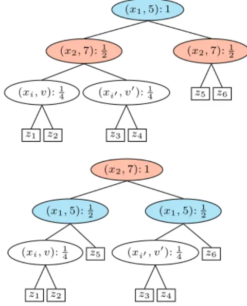
computation. Since all branches of the branch-and-bound algorithm are splits from the GBTs, the GBT lower bounding step bene-fits from branching choices that can fix a larger number of binary variables. We order the splits by preprocessing the GBTs. Each split node contains a split pair(xi, v)and has depthd. Root node hasd= 0. As Fig.2shows, each split node assigns to its(xi, v)pair a weight2−d. A given pair may repeat in a single tree and over different trees. Hence, we sum up all its weights. Sorting the split pairs in non-increasing weight order defines the branch ordering. The choice of2−dfavors split pairs that are higher in their respective GBTs. Branching on such a split pair should be more effective at fixing binary variables. Furthermore, since we sum the weights, the branch ordering also priori-tizes pairs occuring more often. This weighting also incor-porates a fairness property. Assume a GBT where the root splits on (xi1, v1), while both children split on(xi2, v2). Then, these split pairs are interchangable, i.e., (xi2, v2) could be the root and (xi1, v1) the two children. There-fore, they should have the same weight. This idea extends
(x1,5): 1 (x2,7):12 z6 z5 (x2,7):12 (xi′, v′):14 z4 z3 (xi, v):14 z2 z1 (x2,7): 1 (x1,5):12 z6 (xi′, v′):14 z4 z3 (x1,5):12 z5 (xi, v):14 z2 z1
Figure 2. GBT node weighting computed at preprocessing step. Pairs(x1,5)and(x2,7)are interchangeable. So, their summed
weights are equal to ensure the fairness property.
locally to a non-root node. Choosing a local weight of2−d covers this case since the weights are summed up and the GBTs are binary trees. Figure2shows this interchangabil-ity property for an unbalanced tree, where the bottom tree gives a more balanced structure than the top tree.
5.4. Strong Branching
Branch selection is fundamental to any branch-and-bound algorithm. Strong branching selects a branch that en-ables pruning with low effort computations and achieves a non-negligible speed-up in the algorithm’s performance (Morrison et al.,2016). Strong branching is known to have increased the size of efficiently solvable large-scale mixed-integer problems and is a major component of commer-cial solvers (Klabjan et al.,2001;Anstreicher et al.,2002; Anstreicher,2003;Easton et al.,2003;Belotti et al.,2009; Kılınc¸ et al.,2014). We use strong branching to leverage the easy-to-solve convex penalty term for pruning.
At a branch-and-bound nodeS, branching leads in two chil-drenS′ andS′′. One node amongS′ andS′′inherits the convex boundbcvx,S from the parent, while the other re-quires a new computation. We employ strong branching by investigating the kfirst branches in the list generated according to Section5.3. Without loss of generality, sup-pose that S′
does not inheritbcvx,S
. If one of the k pos-sible branches results in bcvx,S′
that satisfies the pruning condition without GBT bound improvement, then it is im-mediately selected as the strong branch and we proceed with nodeS′′
. Figure3 illustrates strong branching. If a strong branch cannot be found, the algorithm performs a lo-cal GBT lower bound improvement (Section5.2.2). If the new local GBT lower bound is not large enough to prune
[(xi1, v1), (xi2, v2), (xi3, v3), . . .] Current Node xi1< v1 xi1≥v1 Current Node xi2< v2 xi2≥v2 Current Node xi3< v3 xi3≥v3 Strong Branch Figure 3. Strong branching for selecting the next spatial branch. A strong branch leads to a node that is immediately pruned, based on a convex bound computation.
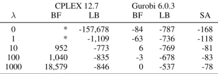
Table 2. Best feasible (BF) solution and lower bound (LB) found by MIQP solvers CPLEX 12.7 and Gurobi 6.0.3 compared with the GenSA simulated annealing solution (SA) with one hour time-out for the industrial instance of Eq. (1).
CPLEX 12.7 Gurobi 6.0.3 λ BF LB BF LB SA 0 * -157,678 -84 -787 -168 1 * -1,109 -63 -736 -118 10 952 -773 6 -769 -81 100 1,040 -835 -3 -678 -83 1000 18,579 -846 0 -537 -78
the current node, the algorithm branches on the first item of the branch ordering, it adds the children to the list of un-explored nodes and continues with the next iteration. The above cases ensure the selection of some branch.
Strong branching allows efficient pruning in regions where the contribution of the convex part in the objective is sig-nificant. Such a branch selection allows early node pruning in the branch-and-bound tree and avoids a large number of useless node repetitions. Furthermore, it reduces the com-putational overhead incurred by bound recalculation. Fi-nally, it results in a sharper bound tightening at a local level.
6. Numerical Analysis
This section compares the Sections 4 and 5 algorithms against black-box solvers. The algorithms are implemented in Python 3.5.3 using Pyomo 5.2 (Hart et al.,2011;2017) for mixed-integer modeling and solver interfacing. We use CPLEX 12.7 and Gurobi 6.0.3. Experiments are run on an Ubuntu 16.04 HP EliteDesk 800 G1 TWR with 16GB RAM and an Intel Core [email protected] CPU.
We test our algorithms on an industrial instance. The con-vex part hasn = 42continuous variables,rank(P) = 2
and|I%|= 37. The GBT part contains 8800 trees where
4100 trees have max depth 16, the remaining trees have max depth 4, the total number of leaves is 93,200 and the corresponding Eq. (3) model has 2061 binary variables. This instance was originally tackled using GenSA
simu-Table 3. Mixed-integer quadratic programming (MIQP), particle swarm optimization (PSO) and simulated annealing (SA) results with a 1 hour timeout.
λ SA MIQP PSO 0 -168.2 -144.0 -150.7 1 -130.7 -104.0 -111.9 10 -102.7 -89.6 -92.0 100 -84.2 -83.2 -85.3 1000 -80.2 -80.4 -76.9
lated annealing package (Xiang et al.,2013) 6.1. Mixed-Integer Quadratic Pragramming
We feed the instance to MIQP solvers CPLEX 12.7, Gurobi 6.0.3 and GenSA simulated annealing package with 1 hour timeout. Table2 lists the obtained results. SA finds bet-ter heuristic solutions than the MIQP solvers. In two cases, CPLEX does not even report a feasible solution. The large optimality gap returned by the MIQP solvers implies that (i) either there exist significantly better solutions than the ones computed by SA, or (ii) the solver lower bounds are extremely weak. Determining a better optimality gap moti-vates the design of our branch-and-bound algorithm. Table 2 shows that the optimization problem is difficult for state-of-the-art commercial MIQP solvers. Moreover, the problem becomes harder as parameterλdecreases and GBTs’ contribution to the objective becomes more signif-icant. This finding motivates the design of optimization methods that aim in bounding efficiently the GBT trained function and exploit bounds on the convex penalty function when its contribution becomes significant. In this last case, we are equipped with stronger bounds.
6.2. Heuristics
We compare the Section4 heuristics to simulated anneal-ing (SA). For MIQP, each iteration introducesN = 10new trees. Table3compares the heuristics for increasingλ. SA outperforms the other heuristics for smallerλ’s and is com-petitive for larger values. Since both MIQP and PSO ex-ploit the convex part, they both perform better for larger values of λ. Figure 4 shows the heuristic improvement over time forλ = 0andλ = 1000. MIQP objective provements are not regular and drop sharply when they im-prove. Particle swarm optimization (PSO) converges to an inferior solution for both λ’s. Even though particles are initially projected towards low penalty regions, they suf-fer from bias, e.g., if a non-optimal solution remains the best found for many iterations, the other particles become biased towards it. For large λ’s, the Section 4 heuristics do not significantly improve on the SA solutions. This
sug-0 0.5 1 −160 −140 −120 −100 Time/hours O b je ct iv e MIQPPSO SA 0 0.5 1 −80 −75 −70 −65 Time/hours O b je ct iv e MIQP PSO SA
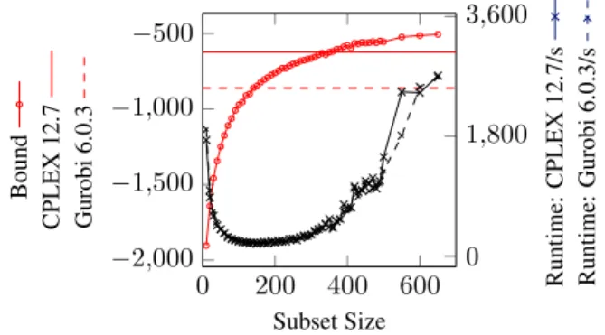
Figure 4. Mixed-integer quadratic programming (MIQP), particle swarm optimization (PSO) and simulated annealing (SA) results. Top:λ= 0. Bottom:λ= 1000. 0 200 400 600 −2,000 −1,500 −1,000 −500 0 1,800 3,600 Subset Size B o u n d C P L E X 1 2 .7 G u ro b i 6 .0 .3 R u n ti m e: C P L E X 1 2 .7 /s R u n ti m e: G u ro b i 6 .0 .3 /s
Figure 5. GBT part bounding using the partition based algorithm (Section5.2). The left axis corresponds to the lower bound and the right axis to the cumulative runtime of CPLEX 12.7/Gurobi 6.0.3 to solve the individual MILPs. The horizontal lines are the CPLEX 12.7 and Gurobi 6.0.3 lower bounds after solving the en-tire instance with one hour time limit.
gests that the Table2lower bounds may be poor motivating the need for an improved bounding approach.
6.3. Branch-and-Bound
The Section5branch-and-bound algorithm initializes with a feasible solution and a GBT part global lower bound. We initialize with the best feasible solutions from Section6.2. For the GBT lower bound, we use the Section5.2approach. We first investigate how different subset sizes affect the cal-culated bound and runtime for this algorithm.
Figure5 compares the GBT bounding algorithm for vari-ous partition subset sizes to MILP solvers CPLEX 12.7 and Gurobi 6.0.3. The bounding algorithm calculates tighter bounds as the subset size increases. For larger sizes, the runtime shows exponential increase. Small subset sizes have a larger computational cost due to the non-negligible modeling overhead of solving many small MILPs.
Compar-0 0.5 1 −1,000 −500 0 Time/hours B o u n d BB-BO BB-WBO Gurobi BF 0 0.5 1 −800 −600 −400 −2000 Time/hours B o u n d BB-BO BB-WBO Gurobi BF
Figure 6. Branch-and-bound lower bound improvement forλ= 0
(top) andλ= 1000(bottom) compared to Gurobi 6.0.3 given a one hour timeout. We test the branch-and-bound algorithm with (BB-BO) and without (BB-WBO) branch ordering. BF is the best known feasible solution.
ing with a black-box approach, we see that a well chosen subset size achieves superior time-to-bound performance. A subset size of 140 solves in 4 minutes and improves on the Gurobi 6.0.3 bound. Choosing a subset size of 360 im-proves on the CPLEX 12.7 bound and takes 8 minutes. Given the Fig.5results, we initialize the branch-and-bound algorithm using a subset size of 150 forProotas it is in the trough of runtime plot. Figure6compares the branch-and-bound algorithm with (BB-BO) and without (BB-WBO) the branch ordering to Gurobi 6.0.3 (solving the entire MIQP problem) and the best known feasible solution for λ= 0andλ= 1000. BB-BO outperforms all of the other approaches, providing a significant decrease in the optimal-ity gap forλ = 1000. Comparing with Gurobi 6.0.3, the λ= 1000case produces a much better optimality gap. For λ = 0, all solvers have a fairly large optimality gap, this is due to the problem being closer to the NP-hard Eq. (3) model Also strong branching is less likely to be invoked in early nodes of the branch-and-bound tree resulting more regular GBT bounds updates and therefore a large increase in cumulative bounding time. Both λ’s show the impor-tance of the branch ordering. BB-BO is able to produce bet-ter bounds earlier and forλ= 1000strong branching cou-pled with the branch ordering results in significant bounds improvement.
7. Conclusion
As machine learning methods mature and their predictive modeling power becomes well-respected industrially, deci-sion makers want to move from solely making predictions on model inputs to deciding algorithmically what is the best model input. In other words, we must move towards optimizing pre-trained machine learning models. This
pa-per effectively addresses a large-scale, industrially-relevant gradient-boosted tree model by directly exploiting: (i) ad-vanced mixed-integer programming technology with strong optimization formulations, (ii) GBT tree structure with pri-ority towards searching on commonly-occurring variable splits, and (iii) convex penalty terms with enabling fewer mixed-integer optimization updates. The particular model application is in chemical catalysis, but the general form of the optimization problem will appear whenever we wish to optimize a pre-trained gradient-boosted tree with convex penalty terms. It would have been alternatively possible to train and then optimize a smooth and continuous machine learning model, but applications with legacy code may start with a GBT. Additionally, it is well known in catalysis that the global solution to an optimization problem is often par-ticularly useful. The methods in this paper not only gener-ate good feasible solutions to the optimization problem, but they also converge towards proving the exact solution.
Acknowledgements
The support of: BASF SE, the EPSRC Centere for Doc-toral Training in High Performance Embedded and Dis-tributed Systems to M.M. (EP/L016796/1), and an EPSRC Research Fellowship to R.M. (EP/P016871/1) is gratefully acknowledged.
References
Anstreicher, K., Brixius, N., Goux, J.-P., and Linderoth, J. Solving large quadratic assignment problems on compu-tational grids. Mathematical Programming, 91(3):563– 588, Feb 2002. ISSN 1436-4646.
Anstreicher, K. M. Recent advances in the solution of quadratic assignment problems.Mathematical Program-ming, 97(1):27–42, Jul 2003. ISSN 1436-4646.
Belotti, P., Lee, J., Liberti, L., Margot, F., and W¨achter, A. Branching and bounds tightening techniques for non-convex MINLP.Optimization Methods and Software, 24 (4-5):597–634, 2009.
Belotti, P., Kirches, C., Leyffer, S., Linderoth, J., Luedtke, J., and Mahajan, A. Mixed-integer nonlinear optimiza-tion. Acta Numerica, 22:1131, 2013.
Bertsimas, D. and Dunn, J. Optimal classification trees.
Machine Learning, 106(7):1039–1082, Jul 2017. ISSN
1573-0565.
Bertsimas, D. and King, A. OR Forum – An algorithmic approach to linear regression. Operations Research, 64 (1):2–16, 2016.
Bertsimas, D. and Mazumder, R. Least quantile regression
via modern optimization.The Annals of Statistics, 42(6): 2494–2525, 12 2014.
Bertsimas, D., King, A., and Mazumder, R. Best subset selection via a modern optimization lens. The Annals of
Statistics, 44(2):813–852, 04 2016.
Bixby, R. E. A brief history of linear and mixed-integer pro-gramming computation. Documenta Mathematica, pp. 107–121, 2012.
Bollas, G. M., Barton, P. I., and Mitsos, A. Bilevel op-timization formulation for parameter estimation in va-porliquid(liquid) phase equilibrium problems. Chem
Eng Sci, 64(8):1768 – 1783, 2009.
Boukouvala, F., Misener, R., and Floudas, C. A. Global op-timization advances in mixed-integer nonlinear program-ming, MINLP, and constrained derivative-free optimiza-tion, CDFO. Eur J Oper Res, 252(3):701 – 727, 2016. Breiman, L., Friedman, J. H., Olshen, R. A., and Stone,
C. J. Classification and Regression Trees. Wadsworth, Inc., 1984.
Chen, T. and Guestrin, C. Xgboost: A scalable tree boost-ing system. InProceedings of the 22nd ACM SIGKDD International Conference on Knowledge Discovery and
Data Mining, pp. 785–794, 2016.
Easton, K., Nemhauser, G., and Trick, M. Solving the travelling tournament problem: A combined integer pro-gramming and constraint propro-gramming approach. In Burke, E. and De Causmaecker, P. (eds.), Practice
and Theory of Automated Timetabling IV, pp. 100–109,
Berlin, Heidelberg, 2003. Springer Berlin Heidelberg. ISBN 978-3-540-45157-0.
Eberhart, R. and Kennedy, J. A new optimizer using par-ticle swarm theory. In Proceedings of the Sixth Inter-national Symposium on Micro Machine and Human Sci-ence, pp. 39–43, Oct 1995.
Freund, Y. Boosting a weak learning algorithm by majority.
Information and Computation, 121(2):256 – 285, 1995.
Friedman, J. H. Greedy function approximation: A gradi-ent boosting machine. The Annals of Statistics, 29(5): 1189–1232, 2001.
Friedman, J. H. Stochastic gradient boosting.
Computa-tional Statistics & Data Analysis, 38(4):367 – 378, 2002.
Hart, W. E., Watson, J.-P., and Woodruff, D. L. Py-omo: modeling and solving mathematical programs in Python.Mathematical Programming Computation, 3(3): 219–260, 2011.
Hart, W. E., Laird, C. D., Watson, J.-P., Woodruff, D. L., Hackebeil, G. A., Nicholson, B. L., and Siirola, J. D.
Pyomo–optimization modeling in Python, volume 67.
Springer Science & Business Media, second edition, 2017.
Hastie, T., Tibshirani, R., and Friedman, J.The Elements of
Statistical Learning. Springer-Verlag New York, second
edition, 2009.
Ke, G., Meng, Q., Finley, T., Wang, T., Chen, W., Ma, W., Ye, Q., and Liu, T.-Y. LightGBM: A highly efficient gradient boosting decision tree. In Guyon, I., Luxburg, U. V., Bengio, S., Wallach, H., Fergus, R., Vishwanathan, S., and Garnett, R. (eds.),Advances in Neural
Informa-tion Processing Systems 30, pp. 3149–3157. Curran
As-sociates, Inc., 2017.
Kennedy, J. and Eberhart, R. Particle swarm optimization.
InProceedings of the IEEE International Conference on
Neural Networks, volume 4, pp. 1942–1948 vol.4, Nov
1995.
Kılınc¸, M., Linderoth, J., Luedtke, J., and Miller, A. Strong-branching inequalities for convex mixed integer nonlin-ear programs.Computational Optimization and
Applica-tions, 59(3):639–665, Dec 2014.
Klabjan, D., Johnson, E. L., Nemhauser, G. L., Gelman, E., and Ramaswamy, S. Solving large airline crew schedul-ing problems: Random pairschedul-ing generation and strong branching. Computational Optimization and
Applica-tions, 20(1):73–91, Oct 2001.
Miˇsi´c, V. V. Optimization of Tree Ensembles. ArXiv
e-prints, 2017. arXiv:1705.10883.
Miyashiro, R. and Takano, Y. Mixed integer second-order cone programming formulations for variable selection in linear regression. European Journal of Operational
Re-search, 247(3):721 – 731, 2015.
Morrison, D. R., Jacobson, S. H., Sauppe, J. J., and Sewell, E. C. Branch-and-bound algorithms: A survey of recent advances in searching, branching, and pruning.Discrete
Optimization, 19:79 – 102, 2016.
Nocedal, J. and Wright, S. J. Sequential Quadratic
Pro-gramming, pp. 529–562. Springer New York, 2006.
ISBN 978-0-387-40065-5.
Singer, A. B., Taylor, J. W., Barton, P. I., and Green, W. H. Global dynamic optimization for parameter estimation in chemical kinetics. J Phy Chem A, 110(3):971–976, 2006.
Snoek, J., Larochelle, H., and Adams, R. P. Practical bayesian optimization of machine learning algorithms.
InAdvances in Neural Information Processing Systems
25, pp. 2951–2959. Curran Associates, Inc., 2012. Sra, S., Nowozin, S., and Wright, S. J. Optimization for
Machine Learning. MIT Press, 2012.
Xiang, Y., Gubian, S., Suomela, B., and Hoeng, J. Gener-alized simulated annealing for efficient global optimiza-tion: the GenSA package for R. The R Journal Volume 5/1, Jun 2013.
Zhang, H., Si, S., and Hsieh, C.-J. GPU-acceleration for Large-scale Tree Boosting. ArXiv e-prints, 2017. arXiv:1706.08359.