Understanding Graph Data Through Deep
Learning Lens
Supriya Pandhre
A Thesis Submitted to
Indian Institute of Technology Hyderabad
In Partial Fulfillment of the Requirements for
The Degree of Master of Technology
Department of Computer Science & Engineering
Acknowledgements
It has been a wonderful journey as a MTech student at IITH, and I was fortunate to share it with very inspiring and exceptionally intelligent people.
First, I would like to express my deepest gratitude to my adviser Dr.Vineeth N Balasubramanian, who has always been very supportive and encouraging throughout my journey. Before joining as his student, I was just a person interested in research with no clue of what exactly it means to do a research. Like a lighthouse guides a lost ship in the big ocean, he guided me. His guidance not only made me a better researcher but also a better person. Everything I could achieve in my career, its because of him.
I would like to thank Dr.Manish Gupta, with whom I was fortunate to have co-authored two papers and learned a lot from him. I would also like to thank Himangi Mittal, who has greatly helped me in getting my first research paper published at the conference. Her dedication and enthusiasm has always inspired me. A big thanksto my friends and group members: Adepu Ravi Sankar, Arghya Pal, Akilesh B, Tanya Marwah, Anirban Sarkar, Joseph K J, Arjun D’Cunha, Bhavana Jain and the list continues. Discussions with them in weekly meetings has helped me hone my research skills, making me push my boundaries and extend my thinking directions.
I am thankful to my parents who has always encouraged me to aim high and supported me in chasing my dream. Thank you for your endless love!
Abstract
Deep neural network models have established themselves as an unparalleled force in the domains of vision, speech and text processing applications in recent years. However, graphs have formed a significant component of data analytics including applications in Internet of Things, social networks, pharmaceuticals and bioinformatics. An important characteristic of these deep learning techniques is their ability tolearn the important features which are necessary to excel at a given task, unlike traditional machine learning algorithms which are dependent on handcrafted features. However, there have been comparatively fewer efforts in deep learning to directly work on graph inputs. Various real-world problems can be easily solved by posing them as a graph analysis problem. Considering the direct impact of the success of graph analysis on business outcomes, importance of studying these complex graph data has increased exponentially over the years.
In this thesis, we address three contributions towards understanding graph data: (i) The first contribution seeks to find anomalies in graphs using graphical models; (ii) The second contribution uses deep learning with spatio-temporal random walks to learn representations of graph trajectories (paths) and shows great promise on standard graph datasets; and (iii) The third contribution seeks to propose a novel deep neural network that implicitly models attention to allow for interpretation of graph classification.
Contents
Declaration . . . ii
Approval Sheet . . . iii
Acknowledgements . . . iv
Abstract . . . v
1 Introduction 1 1.1 Motivation . . . 1
1.2 Contributions & Outline . . . 2
2 Background: Graph Analysis 4 2.1 Graph Outlier Detection . . . 4
2.1.1 Community-based Outlier Detection . . . 4
2.1.2 Analysis of Edge-attributed Graphs . . . 4
2.2 Temporal Graph Analysis . . . 5
2.3 Network Representation Learning . . . 5
2.3.1 Node Classification . . . 5
2.3.2 Graph Classification . . . 6
3 Community-based Outlier Detection for Edge-Attributed Graphs 8 3.1 Motivation . . . 8
3.2 Methodology . . . 10
3.2.1 Problem Statement . . . 10
3.2.2 Cliques and Potentials in HMRF . . . 12
3.2.3 Probability of Generating the Data . . . 13
3.3 Inference . . . 14
3.3.1 Inferring Hidden Labels . . . 14
3.3.2 Estimating Parameters . . . 16
3.4 Discussion . . . 17
3.5 Experiments . . . 17
3.5.1 Synthetic Dataset . . . 18
3.5.2 Four Area Dataset . . . 19
4 STWalk: Learning Trajectory Representations in Temporal Graphs 22 4.1 Motivation . . . 22 4.2 Methodology . . . 23 4.2.1 STWalk1 . . . 24 4.2.2 STWalk2 . . . 25 4.3 Experiments . . . 27 4.3.1 Datasets . . . 27 4.3.2 Baseline Methods . . . 29
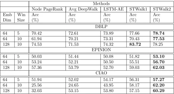
4.3.3 STWalk for Trajectory Classification . . . 29
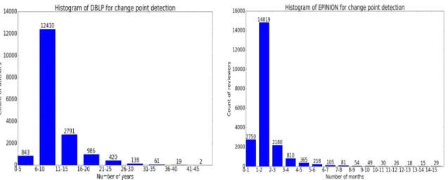
4.3.4 STWalk for Change Point Detection . . . 32
4.3.5 Arithmetic Operations on Trajectory Representations . . . 33
4.4 Conclusion . . . 35
5 Attend, Order and Classify: End-to-End Deep Neural Network for Graph Clas-sification 36 5.1 Motivation . . . 36
5.2 Related Work . . . 38
5.2.1 Learning Permutation . . . 38
5.2.2 Interpretability of Neural Network . . . 38
5.3 Methodology . . . 39 5.3.1 Problem Statement . . . 40 5.3.2 SoftAttention Module . . . 40 5.3.3 SoftOrdering Module . . . 41 5.4 Experiments . . . 43 5.4.1 Datasets . . . 43 5.4.2 Experimental Setup . . . 44 5.4.3 Results . . . 45 5.5 Discussion . . . 46
5.5.1 Using AtOrC for Explaining Network Decisions: . . . 46
5.5.2 Ablation Study . . . 46
5.6 Conclusion . . . 50
6 Conclusions 51
Chapter 1
Introduction
1.1
Motivation
The rising use of social networks and various other sensor networks in real-world applications ranging from politics to healthcare has made computational analysis of graphs a very important area of research today. Study of user-user interactions also plays a crucial role in applications such as user classification for targeted advertising or link prediction to suggest new connections on social networking sites. With increasing amount graph data being generated from diversity of sources, analyzing and understanding the graph data has now gained more importance than ever. In this dissertation, we consider three fundamental graph analysis tasks: anomaly detection in static graphs (arXiv 2016), learning trajectory representation on dynamic graphs (ACM CoDS-COMAD 2018) and end-to-end framework for graph classification (under review at IEEE ICDM 2018). For each of the aforementioned tasks, we developed different models and techniques using deep learning for understanding the complex graph data.
Our first contribution aims at analyzing the static graphs and finding the anomalies. Beyond graph analysis tasks like graph query processing, link analysis, influence propagation, there has recently been some work in the area of outlier detection for information network data. Although various kinds of outliers have been studied for graph data, there is not much work on anomaly de-tection from edge-attributed graphs. In this light, we introduce a method that detects novel outlier nodes by taking into account the node data and edge data simultaneously to detect anomalies. We model the problem as a community detection task, where outliers form a separate community. We propose a method that uses a probabilistic graphical model (Hidden Markov Random Field) for joint modeling of nodes and edges in the network to computeHolistic Community Outliers (HCOut-liers). Thus, our model presents a natural setting for heterogeneous graphs that have multiple edges/relationships between two nodes. EM (Expectation Maximization) is used to learn model parameters, and infer hidden community labels. Experimental results on synthetic datasets and the DBLP dataset show the effectiveness of our approach for finding novel outliers from networks.
In the quest of understanding the graph data, our second contribution addresses the analysis of temporal graphs. Analyzing the temporal behavior of nodes in time-varying graphs is useful for many applications such as targeted advertising, community evolution and outlier detection. Hence, we present a novel approach, STWalk, for learning trajectory representations of nodes in temporal
graphs. The proposed framework makes use of structural properties of graphs at current and previous time-steps to learn effective node trajectory representations. STWalk performs random walks on a graph at a given time step (called space-walk) as well as on graphs from past time-steps (called time-walk) to capture the spatiotemporal behavior of nodes. We propose two variants of STWalk to learn trajectory representations. In one algorithm, we perform space-walk and time-walk as part of a single step. In the other variant, we perform space-walk and time-walk separately and combine the learned representations to get the final trajectory embedding. Extensive experiments on three real-world temporal graph datasets validate the effectiveness of the learned representations when compared to three baseline methods. We also show the goodness of the learned trajectory embeddings for change point detection, as well as demonstrate that arithmetic operations on these trajectory representations yield interesting and interpretable results.
With the unprecedented success of the deep learning techniques, particularly, Convolution Neural Networks (CNN) in computer vision, natural language processing, and speech processing domain, our third contribution seeks to extend and utilize these concepts for understanding graph-structured data. However, applying Convolution Neural Network directly on graph data presents two problems: i) variable number of nodes to process and ii) no unique way of ordering the nodes. Hence, in this work, we propose AtOrC , a novel end to end deep neural network framework that “learns to select” the important nodes as well as “learns to order” them, all in a single pass of the input graph. As the name “Attend, Order and Classify” suggests, the framework contains 3 modules: the SoftAttention module that learns which nodes to attend to, the SoftOrdering module that learns how to order them and the Convolutional Neural Network that learns local features useful for graph classification. Experiments on several standard benchmark datasets demonstrate that the proposed framework, AtOrC , achieves significant improvement on the classification task. Particularly, the algorithm was able to outperform state of the art methods with 10.66% improvement in classification accuracy on IMDB-MULTI dataset. Moreover, the attention maps generated during the classification process by the SoftAttention module can be used for interpreting the decisions made by the framework. These maps give insights into the deep neural network, making it more reliable and usable in risk-sensitive applications such as healthcare.
1.2
Contributions & Outline
The core contribution of this dissertation is three novel frameworks, each one focused on three task. The first framework detects anomalies in static graphs and hence named “HCODA”:Holistic Community Outlier Detection Algorithm, the second method aims at learning graph representa-tion on dynamic graphs and given name “STWalk”: Space-Time Walk, and the final framework is designed for graph classification that learns to attend and order the graph nodes, hence named “AtOrC”:Attend, Order and Classify. The details of the contributions are given below:
• HCODA: Holistic Community Outlier Detection Algorithm
– We look at the community outlier detection problem from a holistic perspective by in-corporating node data, edge data, and the linkage structure. Based on such a view, we propose the problem of detecting novel HCOutliers.
– We model the problem as a community analysis task over a HMRF and provide inference using an EM algorithm.
• STWalk: Space-Time Walk
– We present an unsupervised trajectory learning algorithm that embeds the spatial and temporal characteristics of nodes over a given time window. The algorithm carries out a random walk in a current graph, resulting in a space-walk, as well as in graphs at different time steps, called time-walk. The traversed random walks are then considered as sentences, with nodes as words from a vocabulary.
– We employ the SkipGram [1] network to learn the latent representations of node trajec-tories such that it maximizes the probability of co-occurrence of two nodes within the specified window size.
• AtOrC: Attend, Order and Classify
– There are three modules in our proposed framework: the Soft-Attention module, the Soft-Permutation module and the Convolutional Neural Network. As the name Attend, Order and Classifysuggests, each one performs one task: Attend, Order and Classify respectively. Each of these modules are differentiable, hence allowing backpropagation to be used to train the network. To the best of our knowledge, our proposed framework is the first end-to-end architecture that learns which nodes to focus on and how to order those nodes, in order to help the convolutional layers learn better features and make more accurate decisions on the graph classification task.
– Soft-Attention Module: Our framework uses Soft-Attention over the nodes of the graph to select few important nodes. It is achieved by applying 1D Gaussian filter, whose mean and variance are learned by backpropagation algorithm. We also show that these learned attention maps can be used to interpret the decisions made by the model(figure 5.1).
– Soft-Permutation Module: We also propose the Soft-Permutation network that learns the best ordering of nodes that will help the model to perform better at graph classification task.
– We use the Convolutional Neural Network to learn the local features of the nodes. Instead of selecting only one filter size for the convolution operation, we used Inception Module, inspired by the InceptionNet [2] architecture.
Thesis Outline:
The thesis is divided into six chapters. In Chapter 1, we introduce the graph analysis and provide overview of our contributions. In Chapter 2, we give background on graph analysis. The Chapter 3 presents our work on outlier detection in edge-attributed graphs. In Chapter 4, we propose our contribution in learning representation on temporal graph. In Chapter 5, we present our work on graph classification. Finally, we conclude in Chapter 6.
Chapter 2
Background: Graph Analysis
2.1
Graph Outlier Detection
Outlier detection has a long history and [3, 4, 5] provide extensive overviews of popular methods; [6, 7] focus on network outlier detection methods. Our work is most related to two main sub-areas of network outlier detection: community-based outlier detection and analysis of edge-attributed graphs, each of which is discussed below.
2.1.1
Community-based Outlier Detection
Community-based outlier detection methods perform community analysis on graphs. Nodes that do not belong to any community are labeled as outliers. Community-based outlier detection has been studied both for static networks and dynamic networks. The notion of community outliers has been studied for static bipartite graphs using random walks in [8], for static homogeneous networks using probabilistic models in [9], and for static heterogeneous graphs using non-negative matrix factorization in [10]. [11] summarizes different anomaly detection methods in dynamic graphs such as decomposition based methods [12], [13], distance based methods [14]. Community based outlier detection method, for dynamic graphs, is proposed for a two-snapshots setting in [15] and for a series of snapshots in [16].
2.1.2
Analysis of Edge-attributed Graphs
Edge content indicates the type of relationship between the two nodes. However very little work exists on analysis of edge-attributed graphs. Qi et al. [17] proposed a edge-induced matrix factor-ization based method for finding communities in social graph using edge content. [18] proposed a method that considers edge data of User-Likes-Pages Facebook graph for temporal analysis to find the page-like pattern. [19] proposed a method for mining coherent sub-graphs in multi-layer edges by exploiting edge content. [20] proposed a method for finding top-Kinteresting subgraphs matching a query template where interestingness is defined using edge weights. We propose a community-based outlier detection method for edge-attributed graphs which jointly exploits edge content along with node data and the linkage structure.
2.2
Temporal Graph Analysis
Related to the other focal subarea for this work, time-varying graphs have been studied for appli-cations such as node classification [21, 22, 23], link prediction [24], community evolution [25] and outlier detection [7] in recent years. In one of the earlier works in this area, Tang et al. [25] pro-posed a spectral clustering framework for studying the evolution of communities in time varying multi-mode networks. Aggarwal et al. [21] proposed a node classification model that used network structure and node attributes from time-varying graphs. The model was specifically designed for textual node attributes. In [24], a non-parametric model was proposed for link prediction in a series of network snapshots. More recently, Li et al. [23] presented a framework that used node attributes for learning node embeddings. The model first learns separate embeddings from network structure and node attributes respectively. The node embeddings are then combined using matrix perturba-tion theory. Another recent work, GraphSAGE [22], proposed an inductive algorithm that generates node embeddings using sampling and aggregating local neighborhood information and learning a function to generate node embeddings of unseen data. For more such methods, Aggarwal et al. [26] provide a comprehensive survey on methods for temporal graph analysis.
While there have been a few efforts on analysis of time-varying graphs, all the aforementioned algorithms enforce the data to have node attributes. Many real-world graph data, however, may not provide node features either because they are not available publicly for use or they are missing (for instance, it is optional to fill age or location while creating a user profile on Twitter). In this work, we seek to propose a new framework, SpaceTimeWalk (STWalk), that seeks to utilize only the structural properties of time-varying graphs to learn compact low-dimensional embeddings capturing spatio-temporal properties of node trajectories.
We now present the proposed STWalk algorithm.
2.3
Network Representation Learning
2.3.1
Node Classification
In recent years, there have been a few approaches proposed for learning representations of networks, in particular, learning graph node embeddings. Many of the recent efforts have been inspired by the recent wave of deep learning methods that have demonstrated impressive success in learning representations of other kinds of data such as images, speech and text. DeepWalk [27], one of the earliest efforts in this regard, combined a random walk-based method with a SkipGram network (traditionally used in Natural Language Processing) to learn node representations. Node2vec [28] extended DeepWalk by employing biased random walks to learn node embeddings. In particular, Node2Vec precomputes a matrix, which is similar to a transition probability matrix, that assigns a probability of transition in a random walk, and is based on two hyper-parameters that control whether the walk will stay within a close neighborhood of the node or it will move farther away from that node.
Tang et al. (LINE) [29] computed node embeddings using a function of the probability of observing first-order and second-order nodes together in a random walk within a certain window size. This method then uses Asynchronous Stochastic Gradient Descent to solve the optimization problem. GraRep [30] employed a Singular Value Decomposition-based method for dimensionality reduction
and learning graph representations. Cao et al. [31] proposed a stacked denoising autoencoder for learning the vertex representations in graphs, where they used random surfer model to learn the structural properties of graph calculate the positive pointwise mutual information and then employ denoising autoencoder to reduce the dimensions of learned node features. There have also been efforts, such as [32], which have used deep neural network-based models for learning embeddings in heterogeneous networks. The main goal of the paper [32] was to consider information from multiple sources in dynamic network and learn unified representation. A more detailed review on network embedding techniques can be found in [33]. However, all the aforementioned methods work only with static graphs. In this work, we focus on learning representations of node trajectories in dynamic graphs. Dynamic graphs are evolving by nature, and it is important to capture the addition and deletion of nodes and edges, while capturing the behavior of a node over time in a learnt representation.
Node classification using Attention: Many algorithms have been proposed for node classification. However, recently researchers have started using attention for this task. The main aim of using the attention is to pick only few neighbors whose features are most helpful in discriminating the current node. This problem of focusing on important neighbors is solved by taking a weighted average of neighbors. The algorithms differ in the way they calculate the neighborhood weights. Masci et al [34] propose an algorithm for 3D shapes that works in non-Euclidean domain. The neighborhood weight is calculated based on the distance between two nodes on a polar coordinate system. Boscaini et al [35] use the heat kernel to measure the distance between two nodes and calculate the neighborhood weight. Monti et al [36] propose to learn mixture of Gaussian distributions on the neighborhood that will learn how to weight the neighbors instead of using predetermined weighing function. Velickovic et al [37] propose similar algorithm. Atwood et al [38] proposed a diffusion-convolution operation for node classification. Our work differs from these algorithms as we propose to use attention for graph classification i.e. selecting important nodes out of all the nodes in graph which are helpful in classifying the given graph. Our motivation for using attention is, the real-world graphs can be very huge and hence it is not feasible solution to use all nodes to classify the graph. Moreover, only certain area of graph could be playing important part in distinguishing the graph from others. Hence, in this work we propose SoftAttention module which picks the most important nodes in the graph that will help it classify the graph correctly.
2.3.2
Graph Classification
Early work in the domain of graph classification include kernel based algorithms such as Shortest-path kernel [39], random-walk kernel [40], graphlet count kernel [41] and WL kernel [42]. However, the main issue with these algorithms is they are not scalable and non-differentiable. In recent time, many deep learning based approaches have been proposed. Niepert et al [43] proposed a CNN based architecture for graph classification. The algorithm includes multiple preprocessing steps that coverts the given graph in such a way that CNN can be applied on it. Subgraph2vec [44] algorithm uses information from nearby nodes to learn the latent representation of rooted subgraph in unsupervised setting and these features are then used for graph classification. Deep Graph Kernel [45] count the occurrences of small size graphlets in given graph. It is used as feature vector for graph classification. Zhang et al [46] propose a pooling layer which sorts the nodes and considers first few nodes for graph classification. Our work is different than these algorithm as it is end-to-end differentiable,
with SelfAttention module that selects the most important nodes in the graph, SelfOrdering module that orders the nodes in such a way that it can perform better at graph classification.
Chapter 3
Community-based Outlier
Detection for Edge-Attributed
Graphs
3.1
Motivation
Outlier (or anomaly) detection is a very broad field which has been studied in the context of a large number of research areas like statistics, data mining, sensor networks, environmental science, distributed systems, spatio-temporal mining, etc. Many algorithms have been proposed for outlier detection in high-dimensional data, uncertain data, stream data and time series data. By its inherent nature, network data provides very different challenges that need to be addressed in a special way. Network data is gigantic, contains nodes of different types, rich nodes with associated attribute data, noisy attribute data, noisy link data, and is dynamically evolving in multiple ways. Outlier detection on networks for various applications can be useful for: (1) identification of interesting entities or sub-graphs, (2) data de-noising (both with respect to the network nodes and edges), (3) understanding the anomalous temporal behavior of entities, and (4) identification of new trends or suspicious activities in both static and dynamic scenarios. Some examples of network outliers include users who spread rumors on Twitter, unusual but successful associations of persons with various organizations in an organizational network, sensor with anomalous readings in a sensor network, anomalous traffic between two components in a distributed network, snapshot with broken correlation between network properties across time, etc.
Given a static graph, one can find node, edge or subgraph outliers. For dynamic graphs, the outliers could be time stamps where the properties of the snapshot are significantly different from the properties of other snapshots. In the dynamic scenario, one can also identify a node (or an edge, or a subgraph) which shows anomalous behavior across time as an outlier. Popular outlier detection methods for static graphs include the Minimum Description Length (MDL) method [47], frequent subgraph mining, egonet analysis [48], and community analysis [9, 10]. Popular methods for outlier detection for dynamic graphs include graph similarity based methods [49], temporal spectral analysis [50], temporal structural connectivity analysis [51], and temporal community analysis [16,
15].
While most work in the past on network outlier detection has focused on graphs with node data and links, there is very little work in the area of edge-attributed graphs. In some cases, node data and linkage could be normal even when edge data is abnormal, in the context of nodes on which the edge is incident. With the rich variety of interactions in various complex graphs across a variety of domains, it is critical to incorporate such edge attributes in finding novel outliers. If we could assign a latent community to every node and every edge, a HCOutlier node is one which is linked to many nodes of another community, or has incident edges belonging to another community.
The following real-world examples demonstrate the importance of HCOutliers.
Organizational Graph Example: A graph of people working in a company is called an organization graph. Edges represent frequent communication. Role of a person can be considered as the commu-nity label. Usually a chemist in a company would communicate frequently with other chemists. But a suspicious HCOutlier node would not just communicate frequently with members of other roles, but also the community of the communications would be different from the one expected for its role. Such a person could be an activist planning a malicious activity with other folks in the company, or a star performer working on a secret collaborative project.
Co-authorship Graph Example: A co-authorship graph contains authors as nodes. Two authors are connected if they have published a paper together. On such graphs, research areas can be considered as latent communities. Most authors collaborate with other authors, and publish papers in the same research area. An HCOutlier would be an author who: (1) collaborates frequently with authors from other research areas, and (2) collaborates with other authors of same or different community on papers which belong to other research areas. Such authors perform inter-disciplinary research and are vital in cross-pollination of concepts across research areas.
Co-actorship Graph Example: A co-actorship graph contains actors as nodes. Two actors are con-nected if they have worked in a movie together. On such graphs, movie genres can be considered as latent communities. Most actors collaborate with other actors, and work in moviesin the same genre. An HCOutlier would be an actor who: (1) collaborates frequently with actors from other genres, and (2) collaborates with other actors of same or different genre in movies which belong to other genres. HCOutlier actors are ones who have built a reputation for being multi-faceted actors with an eclectic range of movies.
Limitations of Past Approaches: In the past, various approaches have been proposed by looking only at node data and ignoring network structure. Clearly, HCOutliers cannot be detected using such a global approach because HCOutlier nodes belong to popular communities. There has been work on finding community outliers for both homogeneous [9] and heterogeneous graphs [10] by considering node data and link structure but ignoring edge data. Clearly, such an approach can identify some HCOutliers who are linked to nodes with a different community label. But they cannot identify a HCOutlier who could be connected to nodes of the same community label but has incident edges with a different community label.
Brief Overview of the Proposed Approach: We propose a probabilistic model for detection of Holis-tic Community Outliers. We model the problem as a community detection task where the outliers are modeled as a separate community. A Hidden Markov Random Field (HMRF) is used to perform joint community analysis for both nodes and edges considering node data, edge data and the linkage structure. Thus, the HMRF contains both nodes and edges from the graph as vertices, referred
to as a node-vertex and an edge-vertex respectively. Community labels for outliers are sampled from a uniform distribution while normal vertices could be sampled from Gaussian or a multinomial distribution. EM is used for the inference, and to compute the hidden community labelZ for every vertex.
We make the following contributions in this chapter:
• We look at the community outlier detection problem from a holistic perspective by incorpo-rating node data, edge data, and the linkage structure. Based on such a view, we propose the problem of detecting novel HCOutliers.
• We model the problem as a community analysis task over a HMRF and provide inference using an EM algorithm.
• Using several experiments on synthetic datasets and a DBLP dataset, we show the effectiveness of the proposed approach in identifying HCOutliers.
3.2
Methodology
In this section, we develop the HMRF model which we use to perform joint community analysis for both nodes and edges considering node data, edge data and the linkage structure.
3.2.1
Problem Statement
Consider an undirected graphG={V, E}, where V is the set of vertices andE is the set of edges. Node and Edge Data: LetS be the set of observed data.
• LetSi represent the observed data of nodevi ∈V which haspattributes,Si1,Si2,· · ·,Sip. • LetSij represent the observed data of edge eij ∈E, i.e., edge data between nodesvi andvj,
and there are qnumber of attributes,Sij1,Sij2, · · ·, Sijq.
HMRF Model: The HMRF contains a vertex representing each node and each edge fromG. We refer to the HMRF vertices representing nodes and edges as node-vertices and edge-vertices respectively. We use the index i to refer to node-vertices in the HMRF, and the index ij to refer to edge-vertices in the HMRF. We use the indexb to refer to all the vertices in the HMRF. Thusb∈B= {1,2,· · ·, i,· · ·,|V|,(1,2),(1,3),· · · ,(1,|V|),(2,3),· · ·,(|V| −1,|V|)}. Note thatij ∈ B if i < j. Thus,|B|=|V|+|E|.
• Let X ={Xb} be a set of random variables. Xi generates node dataSi, and Xij generates
edge dataSij.
• LetZ ={Zb} be the set of hidden random variables. Zi indicates the community assignment
of vi. Suppose there are K communities, thenZi ∈ {0,1,2,· · ·, K}. If Zi = 0, thenvi is an
outlier. IfZi=k, thenvi belongs to the communityk. Similarly,Zij denotes the community
• Let W denote the weights in the HMRF. Wvi,vj is set to the weight of the edge eij ∈E and
represent edge strength. Wvi,vj,eij are weights for a triangle clique consisting ofvi,vj andeij.
Thus,|W|= 4|E|(3 faces of the triangle formed by two node-vertices and an edge-vertex, and the whole triangle itself).
Wvi,eij can be set in multiple ways. We set it to the inverse of number of neighbors ofvi in G.
Thus, for a co-authorship graph, this weight can be set to the inverse of the number of co-authors of author vi in the graph. For a Twitter users graph, this weight can be set to the inverse of the
number of other users that the uservi is connected to. In a directed network sense, the weight can
also be set to the ratio of the number of tweets from user vi to user vj to number of total tweets
from uservi.
Wvi,vj,eij should reflect some property of the triangle clique which cannot be captured using
individual edges. For a co-authorship network, this could be set to ratio of number of papers where authorsvi andvj are co-authors to the total number of papers on which eithervi orvj are authors.
Similarly, for a Twitter user network, this weight can be set to the ratio of tweets exchanged between usersvi andvj to the total tweets posted by either vi orvj.
Zb’s are influenced by their neighbors, i.e., if two nodes are linked, it is likely that both belong to
the same community. This does not hold for the outliers. LetNidenote the set of neighbors of node
vi. IfZi = 0, thenvi is an outlier, and so the neighborhood set is empty. Also, each node-vertex is
connected to the edge-vertex corresponding to the edges which are incident on the node inG.
Ni= {vj|Wvivj >0, i6=j, Zj6= 0}∪ {exy|Wviexy >0, x=i or y=i, Zxy6= 0} Zi6= 0 φ Zi= 0 (3.1)
Similarly, we also define neighbors for edge-vertices,Nij, as follows. Note that for an edge-vertex,
the neighbors are only the node-vertices on which the edge-vertex is incident except for the case when these node-vertices are outliers.
Nij =
(
{vi|zi6= 0} ∪ {vj|zj6= 0} Zij6= 0
φ Zij= 0
(3.2)
Data Likelihood: Let Θ ={θ1, θ2, .., θK}be the set of parameters describing the normal communities.
Thus, likelihood for node/edge data can be written as follows.
P(Xb=Sb|Zb=k) =P(Xb=Sb|θk) (3.3)
We assume the outliers follow uniform distribution as we do not know beforehand which elements(node-vertex or edge-elements(node-vertex) are anomalous or what they look like.
whereρ0 is a constant.
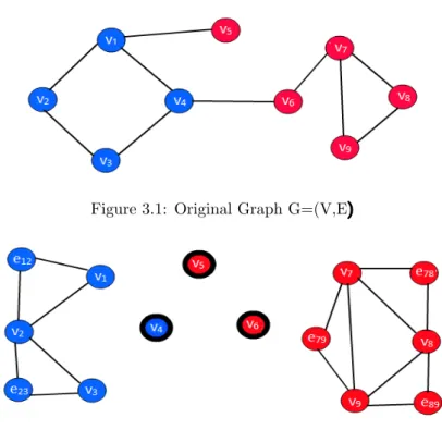
Figures 3.1 and 3.2 illustrate a sample graph and its corresponding HMRF model. The graph has two communities, blue and red. The nodev5has connection with the member of blue community
as if it is part of blue community but its node attributes are similar to red community. Hence, in the HMRF model, it is not connected to any other node, indicatingv5 as an outlier. The edge between
v4 andv6 indicate the cross-community collaboration and thus detected as interesting nodes.
Figure 3.1: Original Graph G=(V,E)
Figure 3.2: HMRF model of G indicating anomalous nodev4,v5andv6
3.2.2
Cliques and Potentials in HMRF
As the community label assignment follows an HMRF, we can defineP(Z) = H1
1exp(−U(Z)) where
U(Z) is the potential function, defined as sum over all possible cliques.
We consider two kinds of clique potentials: pairwise (vi tovj,vi toeij) and triangular (between
U(Z) =−λ1 X Wvivj>0, Zi6=0, Zj6=0 Wvivjδ(Zi−Zj) −λ2 X Wvieij>0, Zi6=0, Zij6=0 Wvieijδ(Zi−Zij) −λ2 X Wvj eij>0, Zj6=0, Zij6=0 Wvjeijδ(Zj−Zij) −λ3 X Wvivj eij>0, Zi6=0, Zj6=0, Zij6=0 Wvivjeijψ(Zi, Zj, Zij) (3.5)
whereλ1, λ2, λ3 are constants,Wvivj >0,Wvieij >0,Wvjeij >0,Wvivjeij >0, imply that there are
links connectingvi-vj,vi-eij,vj-eijandZi,Zj,Zijare non-zero. Theδfunction is defined asδ(x) = 1
ifx= 0 andδ(x) = 0 otherwise. Also,ψ(Zi, Zj, Zij) = 1 ifδ(Zi−Zj) +δ(Zi−Zij) +δ(Zj−Zij)≤1,
and 0 otherwise. Note that we defineψ this way to capture the intuition that the clique potential should fire if at least two of the members in the clique share the same community label. Overall, the potential function suggests that, if members of the clique are normal objects, they are more likely to be in the same community when there exists a link connecting them in G, and the probability becomes higher if their link (weight) is stronger.
3.2.3
Probability of Generating the Data
Given the community label of a vertex (ZiorZij) in the HMRF, the corresponding data (XiorXij)
can be modeled as data generated from a distribution with parameters specific to the community. Community labels can be obtained using either Gaussian mixture model on the data if it is contin-uous, or as multinomial if the data is textual.
Continuous Data: If the data is numeric and 1-dimensional, we need to learn the mean (µk), and
standard deviation (σk) for each communitykrepresented using a Gaussian. Given the parameters
and the community label, the log likelihood can be written as follows.
lnP(Xi=Si|Zi=k) =− (Si−µk)2 2σ2 k −lnσk−ln √ 2π (3.6)
In case of multi-dimensional data withpdimensions, the log likelihood can be written as follows.
lnP(Xi=Si|Zi=k) =− (Si−µk)TΣk−1(Si−µk) 2 −ln Σk 2 −ln p (2π)p (3.7)
attributes (or words) are independent of each other, given the community label. P(Xi=Si|θk) = p Y c=1 P(Xic =Sic|θk) (3.8) P(Xij =Sij|θk) = q Y c=1 P(Xijc=Sijc|θk) (3.9)
For text data, given a vocabulary ofT words, letdbl be the number of times the wordl appears
in data related to vertexb. Then the parameters θk ={βk1,· · ·, βkT} denote the probability of a
particular word belonging to communityk. Given the parameters, the data likelihood of an object belonging to thekthcommunity can be computed as follows.
lnP(Xic =Sic|Zi =k) =
T
X
l=1
dillnβkl (3.10)
whereβkl is the probability of the word with indexl belonging to communityk.
3.3
Inference
The model parameters Θ and the set of hidden labelsZ are unknown as described in Section 3.2. In this section, we describe methods to infer the hidden labels and also estimate the model parameters.
3.3.1
Inferring Hidden Labels
Assuming the model parameters Θ are known, we find the configurationZ that will maximize the posterior distribution as follows.
ˆ
Z = arg max
Z P(X=S|Z)P(Z) (3.11)
To find such a configuration, we use the Iterated Conditional Modes (ICM) algorithm [52]. It is a greedy algorithm which guarantees convergence to a local optima by sequentially updating oneZb
at a time assuming otherZ’s (i.e.,ZB−b) as constant. At each step, the algorithm updatesZb given
Xb =Sb and the other labels such that the posteriorP(Zb|Xb=Sb, ZB−b) is maximized. IfZb 6= 0,
applying Bayes rule,
P(Zb|Xb=Sb, ZB−b)∝P(Xb=Sb|Z)P(Z) (3.12)
In Eq. 3.12,P(Z) can be computed using Eq. 3.5. But rather than considering potential for the entire graph, Eq. 3.12 needs potentials defined over only those cliques in whichZb is involved. Thus,
P(Zi|Xi=Si, ZB−{i})∝P(Xi=Si|Z)× exp(λ1 X vj∈Ni Wvivjδ(Zi−Zj) +λ2 X exy∈Ni Wviexyδ(Zi−Zxy) +λ3 X vj∈Ni, exy∈Ni Wvivjexyψ(Zi, Zj, Zxy)) (3.13)
Also, the corresponding equation for the edge-vertices can be written as follows.
P(Zij|Xij=Sij, ZB−{(i,j)})∝P(Xij=Sij|Z)× exp(λ2 X vi0∈Nij Wvi0eijδ(Zi0−Zij) +λ3Wvivjeijψ(Zi, Zj, Zij)) (3.14)
Taking log of the posterior probability, we can transform the maximizing posterior problem to minimizing the conditional posterior energy function defined as shown in Eqs. 3.15 and 3.16 for node-vertices and edge-vertices respectively.
Ui(k) =−lnP(Xi=Si|Zi=k)−λ1 X vj∈Ni Wvivjδ(k−Zj) −λ2 X exy∈Ni Wviexyδ(k−Zxy) −λ3 X vj∈Ni, exy∈Ni Wvivjexyψ(k, Zj, Zxy) (3.15) Uij(k) =−lnP(Xij=Sij|Zij=k) −λ2 X vi0∈Nij Wvi0eijδ(Zi0−k)−λ3Wvivjeijψ(Zi, Zj, k) (3.16)
IfZb= 0, the vertex has no neighbors, and thus
P(Zb|Xb=Sb, ZB−{b}) ∝ P(Xb=Sb|Zb= 0)P(Zb= 0) (3.17)
Hence,
Ub(0) =−ln(ρ0π0) =a0 (3.18)
Finally, the labelZbfor vertexbin HMRF is set tok∈ {0,1,· · ·, K}such thatUb(k) is minimized.
The predefined hyper-parameters,λ1, λ2, λ3, represent the importance of the respective components
of the graph structure. a0 is the outlierness threshold. Algorithm 8 first randomly initializes the
Algorithm 1: Inferring Hidden Labels
1 Input: Node/Edge dataS, weightsW, set of model parameters θ, number of clustersK,
hyper-parameters (λ1, λ2, λ3), thresholda0, initial assignment of labelsZ(1);
2 Output: Updated assignment of labelsZ;
3 Randomly set Z(0) t←1while Z(t) is not close enough to Z(t−1) do 4 t←t+ 1forb= 1;b≤ |B|;i+ +do
5 Update Zb(t)=k which minimizesUb(k) using Eqs. 3.15, 3.16 and 3.18
6 end 7 end
8 returnZ(t)
3.3.2
Estimating Parameters
In this subsection, we discuss a method for estimating unknownθ from the data. θ describes the model that generates node data and edge data. Hence we seek to maximize the data likelihood
P(X =S|θ) to obtain ˆθ. However, since both the hidden labels and the parameters are unknown and they are inter-dependent, we use expectation-maximization (EM) algorithm (as shown in Algo-rithm 6) to solve the problem. We direct the reader to [9] for details.
The algorithm starts with an initial estimate of hidden labels Z(1). Given the current
configu-ration of hidden labels, we can estimate model parameters as follows. For univariate numeric data,
µ(kt+1) andσk(t+1) are estimated as follows:
µ(kt+1)= P|B| b=1P(Zb=k|Xb =Sb,Θ(t))Sb P|B| b=1P(Zb =k|Xb=Sb,Θ(t)) (3.19) (σk(t+1))2= P|B| b=1P(Zb=k|Xb=Sb,Θ(t))(Sb−µk)2 P|B| b=1P(Zb=k|Xb=Sb,Θ(t)) (3.20)
For text data, given a vocabulary ofT words, letdbl be the number of times the wordl appears
in data related to vertexb. Then, given the current configuration of hidden labels, we can estimate parameters of the multinomial distributionβkl fork∈ {1,· · ·, K} andl∈ {1,· · ·, T} as follows:
β(klt+1)= P|B| b=1P(Zb=k|Xb=Sb,Θ(t))dbl PT l=1 P|B| b=1P(Zb=k|Xb=Sb,Θ(t))dbl (3.21)
Given the updated parameters, the new configuration of hidden labels can be estimated using Algorithm 8 whereP(Zb=k∗|Xb=Sb,Θ(t)) = 1 ifk∗= arg minkUb(k), and 0 otherwise.
In summary, the Holistic Community Outlier detection algorithm shown in Algorithm 6 works as follows. It begins with some initial label assignment of the vertices in the HMRF. In the M-step, the model parameters are estimated using the EM algorithm to maximize the data likelihood, based on the current label assignment. In the E-step, Algorithm 8 is run to re-assign the labels to the objects by minimizing Ub(k)for each HMRF vertex sequentially. The E-step and M-step are repeated until convergence is achieved, and the outliers are the nodes that have 0 as the final estimated labels.
Algorithm 2: Holistic Community Outlier Detection
1 Input: Node/Edge dataS, weightsW, set of model parameters θ, number of clustersK,
hyper-parameters (λ1, λ2, λ3), thresholda0, initial assignment of labelsZ(1);
2 Output: Set of Holistic Community Outliers;
3 Randomly set Z(0) t←1while Z(t) is not close enough to Z(t−1)do
4 M-step: GivenZ(t), update parameters Θ(t+1) according to Eqs. 3.19, 3.20 or 3.21.
E-step: Given Θ(t+1), update the hidden labels asZ(t+1)using Algorithm 8. t←t+ 1
5 end
6 returnthe indices of outliers: {i:Zb(t)= 0, b∈B}
3.4
Discussion
In this section, we discuss how to set the hyperparameters and how to initialize the hidden labels.
Setting Hyperparameters: The HCOutlier detection algorithm has the following hyperparameters: thresholda0, clique importance variables,λ1, λ2, λ3and number of communities K.
λ1, λ2, λ3 indicate the importance of link between two nodes, the importance of link between
edge-vertex and a node-vertex, and the importance of the triangle between the edge-vertex and the node-vertices of which the edge is incident respectively. Ifλs are set to low values, the algorithm will consider only node information for finding the outliers. If their values are set too high, all connected nodes will have the same label, so an upper bound can be set forλ1+λ2+λ3, such that a value
above this bound will result into empty communities. High λ1 will give more importance to the
linkage in the graph. High λ2 will give high importance to consistency between the node data and
edge data in the graph. High λ3 will give high importance to consistency between the edge data
and both the incident nodes in the graph.
The threshold a0 can be replaced by another parameter (percentage of outliers r) as follows.
In Algorithm 8, first calculate ˆZi = arg minkUi(k)(k6= 0) for each i ∈ {1,· · ·,|V|}and then sort
Ui( ˆZi) in non-descending order. Finally, select toprpercentage as outliers.
K represents the number of normal communities. For small value of K, algorithm will find the global outliers, and for large value ofK many local outliers will be detected because of many com-munities. An appropriateKcan be set using a variety of methods like Akaike Information Criterion (AIC), Bayesian Information Criterion (BIC), Minimum Description Length (MDL), etc.
Initialization of labels: Instead of initializing Z randomly, we initialize Z values by clustering the nodes without considering outliers. To overcome local optima issues, we run the algorithm multiple times with different initialization, and choose the one with the largest data likelihood value.
3.5
Experiments
Evaluation of outlier detection algorithms is difficult in general due to lack of ground truth. Hence, we perform experiments on multiple synthetic datasets. We evaluate outlier detection accuracy of the proposed algorithm based on outliers injected in synthetic datasets. We evaluate the results on real datasets using case studies. We perform comprehensive analysis of objects to justify the top
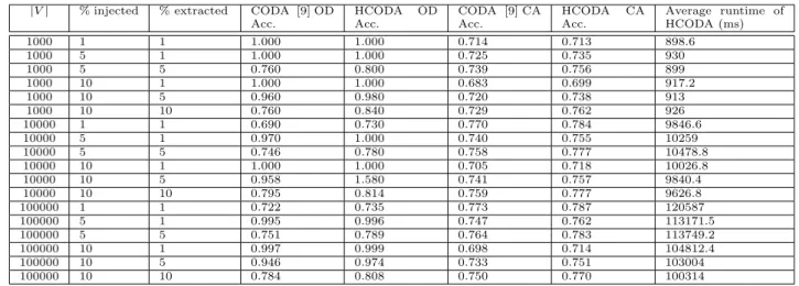
Table 3.1: Synthetic Dataset Results on Graphs A, B and C (K=5; OD Acc.=Outlier Detection Accuracy, CA Acc.=Community Assignment Accuracy; CODA is Baseline, HCODA is the proposed algorithm)
|V| % injected % extracted CODA [9] OD
Acc. HCODA OD Acc. CODA [9] CA Acc. HCODA CA Acc. Average runtime of HCODA (ms) 1000 1 1 1.000 1.000 0.714 0.713 898.6 1000 5 1 1.000 1.000 0.725 0.735 930 1000 5 5 0.760 0.800 0.739 0.756 899 1000 10 1 1.000 1.000 0.683 0.699 917.2 1000 10 5 0.960 0.980 0.720 0.738 913 1000 10 10 0.760 0.840 0.729 0.762 926 10000 1 1 0.690 0.730 0.770 0.784 9846.6 10000 5 1 0.970 1.000 0.740 0.755 10259 10000 5 5 0.746 0.780 0.758 0.777 10478.8 10000 10 1 1.000 1.000 0.705 0.718 10026.8 10000 10 5 0.958 1.580 0.741 0.757 9840.4 10000 10 10 0.795 0.814 0.759 0.777 9626.8 100000 1 1 0.722 0.735 0.773 0.787 120587 100000 5 1 0.995 0.996 0.747 0.762 113171.5 100000 5 5 0.751 0.789 0.764 0.783 113749.2 100000 10 1 0.997 0.999 0.698 0.714 104812.4 100000 10 5 0.946 0.974 0.733 0.751 103004 100000 10 10 0.784 0.808 0.750 0.770 100314
few outliers returned by the proposed algorithm. The code and the data sets are publicly available1.
All experiments are performed on a machine with Intel core i3-2330M processor running at 2.20GHz and 4GB RAM.
We compare our algorithm with Community Outlier Detection Algorithm (CODA) [9]. CODA is also an algorithm for community-based outlier detection which performs community detection using node data and linkage; but ignores edge-data completely.
3.5.1
Synthetic Dataset
We synthetically generate three graphs: Graph A (|V|=1000), Graph B (|V|=10000) and Graph C (|V|=100000). The node data is generated using 5 different Gaussian distributions and similar procedure is followed to generate edge data as well. Then for each of these graphs, different per-centage of outliers are injected by randomly changing the data associated with 1%, 5% and 10% of the nodes.
We generate a variety of synthetic datasets by varying the number of nodes in the graph, per-centage of outliers injected in the graph and perper-centage of outliers to be extracted by the algorithm. Table 3.1 shows the synthetic dataset results for the baseline (CODA) as well as the proposed al-gorithm (HCODA). We set the number of clusters (K) to 5 for these experiments (based on the generation process). We measure the performance of the two algorithms from two perspectives: firstly, accuracy of extraction of the injected outliers (OD Acc.) and secondly, how well it assigns the community label to all the nodes of the graph (CA Acc.). Note that each cell of the table corresponds to average over five runs of the algorithm. As the table shows, the proposed algorithm (HCODA) is 6.2% more accurate than the baseline on average in terms of outlier detection accuracy. Similarly, HCODA is 2.2% better than CODA on average. The performance is consistent across var-ious graph sizes as well as across different degrees of outlierness in the graph.
Hyperparameter Sensitivity: To understand the impact of various hyperparameters (λ’s), we per-formed a few experiments. The results are shown in Figures 3.3, 3.4 and 3.5. Figure 3.3 shows the sensitivity of the outlier detection accuracy with respect to variation ofλ3. We plot the curves for
Graph A and B for the case of 10% injected outliers and 10% outliers to be extracted. Recall that
λ3 is the weight for the triangular clique. As can be seen from the figure, higher values of λ3 are
preferable but in general any value greater than 0.5 is reasonable.
0.74
0.76
0.78
0.8
0.82
0.84
0
0.2
0.4
0.6
0.8
1
Outlier Det
ection
Accur
acy
λ
3Sensitivity of λ
3Graph A
Graph B
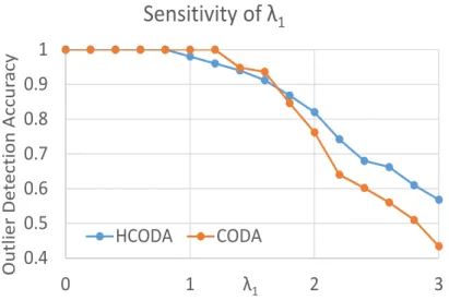
Figure 3.3: Sensitivity ofλ3Figures 3.4 and 3.5 show the sensitivity of the outlier detection accuracy with respect to variation ofλ1 for both the proposed algorithm (HCODA) and the baseline (CODA). Figures 3.4 is the plot
for Graph A while Figures 3.5 is the one for Graph B. Both the plots are for the case of 10% injected outliers and 1% outliers to be extracted. Recall thatλ1 is the weight for the linkage in the original
graph. As can be seen from the figure, lower values ofλ1 are preferable both in the case of CODA
as well as HCODA.
We noticed that the algorithm is not significantly sensitive to the parameterλ2and hence we do
not show the corresponding plot.
3.5.2
Four Area Dataset
DBLP (http://dblp.uni-trier.de/) contains information about computer science journals and proceedings. Four Area is a subset of DBLP for the four areas of data mining (DM), databases (DB), information retrieval (IR) and machine learning (ML). It consists of papers from 20 conferences (five per area): KDD, PAKDD, ICDM, PKDD, SDM, ICDE, VLDB, SIGMOD, PODS, EDBT, SIGIR, WWW, ECIR, WSDM, IJCAI, AAAI, ICML, ECML, CVPR, CIKM. Thus, we consider the authors who have published papers in these conferences, and work with the co-authorship network (edge weight = co-authorship frequency). The edge data consisted of a vector of size four representing the count of papers co-authored in a particular research area.
The graph contains a total of 42844 author nodes. Each author is associated with a vector of size 20 containing the count of papers published by an author in the twenty conferences. There is an
0.74
0.76
0.78
0.8
0.82
0.84
0
0.2
0.4
0.6
0.8
1
Outlier Det
e
ction
Accur
a
cy
λ
3Sensitivity of λ
3Graph A
Graph B
0.4
0.5
0.6
0.7
0.8
0.9
1
0
1
2
3
Outlier Det
e
ction
Accur
a
cy
λ
1Sensitivity of λ
1HCODA
CODA
0.4
0.5
0.6
0.7
0.8
0.9
1
0
1
2
3
Outlier Det
e
ction
Accur
a
cy
λ
1Sensitivity of λ
1HCODA
CODA
Figure 3.4: Sensitivity ofλ1(Graph A)
edge between two authors if they co-authored a paper together and the count of such co-authored papers is the weightWvivj between two nodes.
The graph contains 118618 co-authorship edges. The weight of the link between the author-vertex and the co-authorship-edge-vertex in the HMRF (i.e.,Wvieij) is set to the inverse of the number of
co-authors of authorvi in the graph. Wvi,vj,eij is set to ratio of number of papers where authorsvi
andvjare co-authors to the total number of papers on which eithervi orvjare authors. We set the
number of communities to K=4 (i.e., four normal communities and an outlier community). Also, we set the percentage of outlier parameterr as 1%. The average execution time of the lgorithm is 30.32 seconds.
Case Studies: Result of algorithm show that it is able to identify interesting nodes(authors) and edges(co-authorship). We validate the result produced by algorithm by manually visiting the au-thors’ homepages. For example, work by Sameer K. Antani is mainly in Clinical data standards and electronic medical records, but he published a paper with authors working in information retrieval i.e. node data of Sameer K. Antani is different from the fellow co-authors but the relationship is similar to what two authors from information retrieval should have and hence the algorithm has identified this node as interesting one. Similarly, Ivo Krka mainly focuses on software engineering and system modeling, however, he has published a paper on data mining and hence identified by the algorithm.
The proposed algorithm also identified authors based on the edge information. We discuss a few cases now. Anindya Datta usually publishes in information systems, and Debra E. VanderMeer usually publishes work related to design science research, but their co-authored work is published on data management and very large databases topics. Sabyasachi Saha has co-authored papers with Sandip Sen on topics related to artificial intelligence and he has also published work on information and knowledge management with Pang-Ning Tan. The algorithm was able to identify him because of his work in multiple research areas.
0.74
0.76
0.78
0.8
0.82
0.84
0
0.2
0.4
0.6
0.8
1
Outlier Det
e
ction
Accur
a
cy
λ
3Sensitivity of λ
3Graph A
Graph B
0.4
0.5
0.6
0.7
0.8
0.9
1
0
1
2
3
Outlier Det
e
ction
Accur
a
cy
λ
1Sensitivity of λ
1HCODA
CODA
0.4
0.5
0.6
0.7
0.8
0.9
1
0
1
2
3
Outlier Det
e
ction
Accur
a
cy
λ
1Sensitivity of λ
1HCODA
CODA
Figure 3.5: Sensitivity ofλ1 (Graph B)
3.6
Conclusion
In this chapter, we introduced a method (HCODA) that detects novel Holistic Community Outlier graph nodes by taking into account the node data and edge data simultaneously to detect anomalies. We modeled the problem as a community detection task using a Hidden Random Markov Model, where outliers form a separate community. We used ICM and EM to infer the hidden community labels and model parameters iteratively. Experimental results show that the proposed algorithm con-sistently outperforms the baseline CODA method on synthetic data, and also identifies meaningful community outliers from the Four Area network data.
Chapter 4
STWalk: Learning Trajectory
Representations in Temporal
Graphs
4.1
Motivation
The rising use of social networks and various other sensor networks in real-world applications rang-ing from politics to healthcare has made computational analysis of graphs a very important area of research today. The use of machine learning for various graph analysis tasks such as community detection [53], link analysis [54], node classification [55] and anomaly detection [56] has exponen-tially increased over the last few years, considering the direct impact of the success of these methods on business outcomes. A wide variety of methods have been proposed in the aforementioned areas over the last few years. However, a large part of the efforts so far has focused on static graphs. Platforms such as Facebook, Twitter and LinkedIn correspond to graphs that change on a daily basis; however, the algorithms that analyze such graphs are primarily static, i.e., they consider a graph at a given snapshot of time for analysis. In this work, we seek to focus on temporal graphs, and on learning representations of node trajectories in such graphs.
Study of user-user interactions over time plays an important role in many applications, including user classification for targeted advertising or link prediction to suggest new connections on social networking sites. One of the crucial part of such applications is analyzing change in users’ behavior over time. Aggarwal and Subbian [26] present a survey of methods that have been proposed so far to study temporal graphs, and categorize such methods into two kinds: maintenance methods that focus on adapting older models to a newer version of the same graph, oranalytical evolution analysis, where the objective is to analyze the network as it changes itself. We propose to address the latter in this work. Recent efforts for analysis of temporal graphs have largely extended earlier methods proposed on static graphs, such as spectral methods or those that study statistical properties. In this work, we build on the recent emphasis on learning appropriate representations of data to temporal graphs. In particular, we propose SpaceTimeWalk (STWalk), which learns representations of node trajectories in temporal graphs. To the best of our knowledge, this is the first such effort.
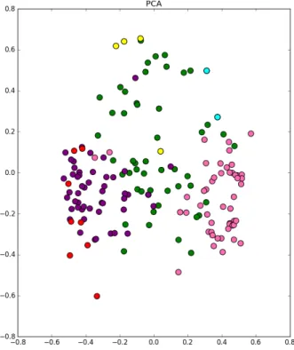
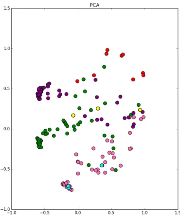
STWalk is an unsupervised trajectory learning algorithm that embeds the spatial and temporal characteristics of nodes over a given time window. The algorithm carries out a random walk in a current graph, resulting in aspace-walk, as well as in graphs at different time steps, calledtime-walk. The traversed paths are then considered as sentences, with nodes as words from a vocabulary. The SkipGram [1] network is then employed to learn the latent representations of node trajectories such that it maximizes the probability of co-occurrence of two nodes within the specified window size. We perform extensive experimentation on three real-world time-varying networks. Performance on these datasets show the effectiveness of our framework in dealing with different kinds of temporal networks. We also study the usefulness of these representations through visualization, as well as complementary tasks such as change point detection.
The remainder of this section is organized as follows. Section 4.2 presents the mathematical formulation of the problem, and the proposed methods are presented in Sections 4.2.1 and 4.2.2. The experimental results that study the performance of the proposed methods are described in Section 5.4, and Section 4.4 concludes the work with pointers to future directions.
4.2
Methodology
Learning the change in behavior of nodes in a temporal graph requires us to consider the information from the graph in the current time step, as well as graphs from previous time steps. Using the na¨ıve way of examining graphs at each time-step separately will fail to capture the correlation information that exists between two graphs at consecutive time steps. Hence, we propose STWalk a random walk based framework that learns rich trajectory representations by capturing changes in node behavior across a given time window. We hence define the following to formulate our solution.
• Given a graphG= (V, E) atT different time steps{G1, G2, G3,· · · , GT}havingN number of
nodes at each time step and varying number of edgesEt, t∈ {1,· · ·, T}, whereEt represents
the edges inGt.
• Let W denote the adjacency tensor of sizeN ×N×T, representing the adjacency matrix of the graph at different time stamps.
Our goal is to learn representations Φ that maps a given node to ad-dimensional representation. LetNt(u)⊂V denote the set of neighbors of node uin graph Gt. For a node uin graph Gt, the
representation Φt(u) will be learned in such a way that, it maximizes the probability of observing
the neighbors ofuin graphGt, viz. Nt(u), and also the representation ofuat previous time stamps
Φt−τ(u) whereτ ∈ {1,· · ·, t−1}. Equation (4.1) below formalizes this construction. Our objective
hence is to obtain ad-dimensional representation for a nodeuat timetthat maximizes the following log probability: max φt X u∈V log Pr (Nt(u), φt−τ(u)|φt(u))) (4.1) whereτ∈ {1,· · ·, t−1}
We assume that the neighborhood nodes inNt(u) and past representationsφt−τ(u) are
log (Pr(Nt(u), φt−τ(u)|φt(u))) = log Y ni∈Nt(u) Pr(ni|φt(u)) + log (Pr(φt−τ(u)|φt(u))) (4.2)
Learning representations using random walk has proved to measure better graph proximity, and thereby improving the performance [33] [57]. Hence, we use random walk to learn the conditional probability of observing a nodeni given the learned representationφt(u) defined as follows:
Pr(ni|φt(u)) = exp(φt(ni)φt(u)) P v∈Nt(u) exp(φt(v)φt(u)) (4.3)
Therefore, to learn the trajectory representation, we maximize:
max φt X u∈V log Y ni∈Nt(u) exp(φt(ni)φt(u)) P v∈Nt(u) exp(φt(v)φt(u)) + log (Pr(φt−τ(u)|φt(u))) (4.4)
While the above problem appears to be learning only the representation of a node at timet, it actually represents a representation of a nodet considering its history over the graphs at the previous time steps, and hence, the termnode trajectory representation in this work.
To solve the maximization problem defined in Equation 4.4, we propose two approaches. The first approach solves equation 4.4 by considering it as one single expression and learning a trajectory representation by maximizing the co-occurrence of neighborhood nodes at timetand in previoust−τ
time-steps together. In the second approach, we learn the trajectory representation by solving two sub-problems separately: (i) maximizing the co-occurrence probability of a node and its neighbors at timet, and (ii) maximizing the co-occurrence probability of a node and its neighbors at preceding
t−τ time-steps. The representations learned using these steps are then combined to form the final trajectory representation. Sections 4.2.1 and 4.2.2 describe each of the proposed approaches.
4.2.1
STWalk1
We describe the first approach, which we call STWalk1, in this section. For learning the trajectory representations of nodes in temporal graphs, here, we take into account the neighbors of a node at time stepst,t−1,..t−τ together and maximize the probability of observing these nodes together. In STWalk1, to consider the neighbors of a nodeufrom the current graph and graphs at previous time steps, we construct a Space-Time Graph. The space-time graph contains all nodes from graph at timetand it has a special temporal edge that links the node to itself in the graphs at previous time steps. Figure 4.1 illustrates this with an example of a space-time graph considered while learning the trajectory representation for node at time t, ut. In particular, the figure shows the temporal
edge (shown as a bold line) between ut and past self-nodes ut−1, ut−2 and ut−3. The trajectory
representation thus learned forutwill hence be influenced by all the nodes in the Space-Time graph,
Figure 4.1: Example graph of node u t generated by Algorithm createSpaceTimeEmb 3. The node
ut represents node in current graph and nodes u(t−1), u(t−2) and u(t−3) indicate its past
self-nodes. To learn trajectory representation foru t, STWalk1 algorithm considers the influence of nodes in current time step as well as effect from the past.
first-level neighbors. Given a node and the window size, over which we want to learn the trajectory, Algorithm 3 describes the steps to create a Space-Time Graph starting from the given node.
Now, to learn the representations of nodes in the Space-Time graph, we perform random walks on it. If two nodes share many edges or neighbors, they will be visited more often in many random walks, indicating that these two nodes share a similar graph structure. Hence, the representation learned for these two nodes should be close to each other in the embedding space. This is analogous to the concept from Natural Language Processing (NLP) that if two words co-occur in many sentences, this indicates that they represent a similar context and hence their word vectors are nearby each other in word embedding space. To learn such a embedding that captures the relationship of a word with other co-occurring words in a window, Mikolov et al. [1] presented the SkipGram network. We use a similar SkipGram algorithm (given in Algorithm 4) to learn the node embeddings from random walks of a graph, similar to DeepWalk [27]. For more details of the SkipGram network, we request the interested reader to refer to [1].
For each node in the Space-Time graph, we performρnumber of random walks each of lengthL. The problem of learning the trajectory representation in such a way that it maximizes probability of co-occurrence of present and past nodes is reduced to maximizing the co-occurrence of nodes in a random walk within a vocabulary windowWv. Hence, we use the SkipGram algorithm 4 to learn
the trajectory representations for nodes. (In particular, we use the SkipGram network, as proposed in [1] to implement the SkipGram algorithm.) For each node in a graphGt, two representations will
be learned. One representation corresponds to the node embedding when it occurs in the context of other nodes, and the other representation which is learned for the node itself. The latter one is used as the node trajectory representation. The overall algorithm STWalk1 is illustrated in Algorithm 5.
4.2.2
STWalk2
In this section, we detail the second approach for learning the trajectory representation of nodes in a temporal graph. We solve the problem of learning representations of node trajectories, such
Algorithm 3: createSpaceTimeGraph
Input: Set of graphsG:{Gt, Gt−1,· · ·, Gt−τ}, Time window sizeτ, starting nodestartN ode
at timet
Output: Gspacetime
1 Gspacetime =Gt
2 foreach time step i∈ {0,· · ·, τ} do 3 pastN ode=startN odeat Gt−i
4 CreatepastN odeSubGraph= the subgraph of pastN odeand its direct neighbors from
Gt−i
5 MergeGspacetime andpastN odeSubGraphto obtain updated Gspacetime
6 startN ode=pastN ode 7 end
Algorithm 4: SkipGram
Input: Input representation: Φ, List of nodes in a random walk: walk, windowSize: Wv
Output: Updated representation: Φ
1 forn∈walkdo 2 forni∈walk[n− Wv,n+Wv] do 3 J(Φ[n]) =−log Pr(Φ[ni]|Φ[n]) 4 Φ[n] = Φ[n]−∂J∂(Φ[Φ[nn]]) 5 end 6 end
that these representations are influenced by present and past neighbors, by dividing it into two sub-problems. We learn the spatial representation from the current graph, Gt, and the temporal
representation from past graphs Gt−1,· · ·, Gt−τ, separately. The final trajectory representation is
obtained by combining the spatial and temporal representations of a given node.
The STWalk2 algorithm first performs a random walk in the current time step graphGt, called as
SpaceWalk, and learns the spatial representation for each node using the SkipGram algorithm. Φspace u,:
corresponds to the learned spatial representation of nodeu. To learn the temporal representation of a node, STWalk2 constructsGnew, which contains only one node from current graph and neighbors
from past graphs. For example, in order to construct such a Gnew in Figure 4.1, we remove all
neighbors from current time-step graph of nodeut. The remaining graph will haveutlinked only to
past subgraphs ofut−1,ut−2andut−3. This will be used asGnewto learn the temporal representation
(in a manner similar to learning the spatial representation above).
The random walks on Gnew capture the temporal relationship between the current node and
nodes from its past graphs. Φtime
u,: corresponds to the learned temporal representation of node
u. Finally, the two learned embeddings are combined to get trajectory representation of nodes. Algorithm 6 summarizes this approach. Line 15 of Algorithm 6 states that the final trajectory representation is a function of spatial and temporal representations. In this work, we found vector addition to work very well in practice in the experiments.
Thus, in STWalk2, we ensure that the trajectory representation of the current node ut has
influence from past nodes by learning the temporal representation explicitly. Learning the temporal representation separately forces the random walk to explore the past graphs of the same node and capture the temporal information between the current node and its past. Therefore, STWalk2 is
Algorithm 5: STWalk1
Input: Given noden∈[1, N], time stept∈[1, T],
length of random walk: L, temporal window size: τ, vocabulary window size: Wv,
Set of graphsG:{Gt, Gt−1,· · · , Gt−τ}, size of embedding: d,
number of restarts (starts at same node): ρ
Output: Updatednthrow of matrix of Φtof size: N×d
1 Initialize Φt[n]∈Rd
2 fori=0 toρdo
3 new graph = createSpaceTimeGraph(G,τ,n) 4 spaceTimeWalk = randomWalk(new graph,n,L); 5 Φt[n] = SkipGram (Φt, spaceTimeWalk,Wv);
6 end
able to learn richer trajectory embeddings than STWalk1 because in STWalk1 we consider the present and past neighbors together, giving the random walks an option of skipping few nodes from past graphs. Experimental results in Table 4.2 validate that the trajectory embeddings learned by STWalk2 perform better than embeddings learned by STWalk1. We now present details of our experiments.
4.3
Experiments
We discuss details of our datasets in Section 4.3.1. We evaluated the proposed methods primarily on the task of trajectory classification. We also extended this to study the goodness of the learned tra-jectory representations through visualization as well as a second task, change point detection. Their performance is compared with three baseline methods, which are described in Section 4.3.2. Section 4.3.3 and 4.3.4 provide the details of the experimental setup and results for the trajectory classifi-cation and change point detection tasks respectively. The code and datasets used for experiments are available on github1.
4.3.1
Datasets
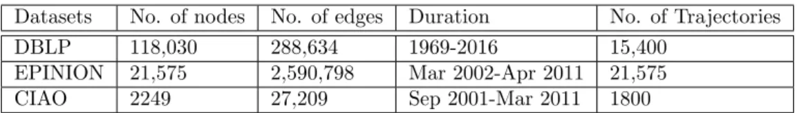
We use three real-world datasets with temporal graphs for the experiments in this work. Each of these datasets is described below.
DBLP Dataset: The DBLP2 dataset contains bibliographic information about a large collection
of computer science publications. This is a dataset commonly used in graph analysis. We have considered a subset of publications which fall under four areas of research: Database, Artificial Intelligence, Data Mining and Information Retrieval. We construct graphs from the this subset of DBLP dataset by considering authors as nodes and connecting two nodes if the corresponding authors have published a paper together. We constructed 45 such annual graphs starting from year 1969 till 2016, excluding years 1970, 1972 and 1974 (whose data was not available on the DBLP
1https://github.com/supriya-pandhre/STWalk 2https://www.informatik.uni-trier.de/ ley/db/