DOI 10.1007/s11721-016-0122-5
Medoid-based clustering using ant colony optimization
Héctor D. Menéndez1 ·Fernando E. B. Otero2 · David Camacho3
Received: 11 November 2014 / Accepted: 9 April 2016 / Published online: 9 May 2016 © The Author(s) 2016. This article is published with open access at Springerlink.com
Abstract The application of ACO-based algorithms in data mining has been growing over the last few years, and several supervised and unsupervised learning algorithms have been developed using this bio-inspired approach. Most recent works about unsupervised learn-ing have focused on clusterlearn-ing, showlearn-ing the potential of ACO-based techniques. However, there are still clustering areas that are almost unexplored using these techniques, such as medoid-based clustering. Medoid-based clustering methods are helpful—compared to classi-cal centroid-based techniques—when centroids cannot be easily defined. This paper proposes two medoid-based ACO clustering algorithms, where the only information needed is the dis-tance between data: one algorithm that uses an ACO procedure to determine an optimal medoid set (METACOC algorithm) and another algorithm that uses an automatic selection of the number of clusters (METACOC-K algorithm). The proposed algorithms are compared against classical clustering approaches using synthetic and real-world datasets.
Keywords Ant colony optimization ·Clustering·Data mining·Machine learning·
Medoid·Adaptive
1 Introduction
Clustering is one of the most relevant areas in data mining and machine learning (Larose 2005;Witten and Frank 2005). Clustering techniques are based on the extraction of patterns in data blindly, referred to as unsupervised learning. Using clustering techniques, data analysts are able to extract information from different datasets without human or expert supervision.
B
Fernando E. B. Otero [email protected]1 Department of Computer Science, University College London, London WC1E 6BT, UK 2 School of Computing, University of Kent, Chatham Maritime, Kent ME4 4AG, UK
3 Department of Computer Science, Universidad Autónoma de Madrid, C/ Tomás y Valiente 11, 28049 Madrid, Spain
Clustering has been designed to group data by similarity. The aim is to minimize the value of a pre-defined cost function, assigning data instances to different groups (clusters) and optimizing this assignment in order to obtain the lowest value of the cost function.
There are several areas that have dealt with clustering problems. One of the most relevant is the statistics area, where well-known clustering algorithms have been proposed, such as K-means, expectation maximization (EM), hierarchical, spectral and fuzzy clustering, among others. Over the last few years, bio-inspired algorithms have received increasing attention. The potential that swarm intelligence and evolutionary algorithms have in optimization has made them potential techniques for clustering. This paper explores this potential, specifically
focusing on ant colony optimization (ACO;Dorigo and Stützle 2004).
The proposed algorithms address the main problem with centroid-based approaches, that is the fact that they need to know the features of the search space in order to determine the central point and that they are sensitive to noise. This means, centroid-based clustering algorithms use a multi-dimensional space to represent the data based on their features in order to find the centroid (central point) position of each cluster. A distance metric (in most cases Euclidean) is used to set a centroid and optimize its position according to the distance between the centroid and the data. As a centroid position is determined by averaging the coordinate values of the data in each cluster, this process does not cope well with outliers. Centroid-based clustering algorithms work well when the data can be represented by features in a multi-dimensional space, e.g. clustering of houses based on features such as price, square metres, number of bedrooms/bathrooms, distance to public transportation. However, they are not appropriate in cases where the features of the data are not clear, e.g. clustering of face images—while it is straightforward to calculate the similarity of images, it not easy to define features to represent them in a multi-dimensional space.
Medoid-based clustering algorithms are usually more robust to noise effects, and data instances do not need to be represented in a multi-dimensional space. They use a notion of similarity/distance among the data instances, which can be obtained as a Gram matrix of a kernel or a distance measure, and they choose data instances to define clusters centres—the selected instances are called medoids.
This paper proposes two medoid-based ACO clustering algorithms, where the only infor-mation needed is the distance among data: one algorithm that uses an ACO procedure to determine an optimal medoid set (METACOC algorithm) and another algorithm that addi-tionally uses an automatic selection of the number of clusters (METACOC-K algorithm). These algorithms use a graph-based structure and a search strategy that requires no knowledge about the search space features. As aforementioned, this strategy is different from classical centroid-based approaches, where the position of the centroid is optimized in order to define the different clusters. In order to evaluate the performance of the proposed algorithms, we have compared them against the ACO-based ACOC algorithm (Kao and Cheng 2006) using synthetic and real-world datasets, and also against five well-known clustering algorithms:
K-means (MacQueen 1967), partition around medoids (PAM;Kaufman and Rousseeuw 1987),
PAMK (Kaufman and Rousseeuw 2009), EMBIC (Fraley and Raftery 2007) and Clues (Wang et al. 2007).
The remainder of this paper is organized as follows. Section2 presents related work,
discussing the clustering problem and previous ACO algorithms for clustering. Section3 introduces the proposed algorithms. Computational experiments and analysis of the obtained
2 Related work
Data mining and machine learning techniques have been used for several applications. One of the most prominent application areas is the identification of patterns in data, which helps data analysts to extract hidden information from data (Larose 2005). Recent data analysis demands have presented new challenges for machine learning techniques (Cao 2010); for example, the need for creating new scalable and robust methodologies is currently receiving increasing interest. In order to improve the robustness of these analysis, new methodologies based on swarm intelligence have shown promise due to the quality of the results extracted using these techniques, which are highly competitive when compared with classical algorithms.
One of the most successful swarm intelligence techniques is ACO (Dorigo and Stützle 2004). ACO algorithms are based on some aspects of the foraging behaviour of ants that collectively can find the shortest path from the nest to a food source. The use of ACO has been extended to several optimization areas, including machine learning. This section provides a general description of the clustering problem—including a discussion of issues about the K-adaptive problem within clustering—and it discusses ACO applications in clustering and the related classification task.
2.1 The clustering problem
Clustering has been widely used in several interdisciplinary areas, such as image segmen-tation (Menéndez et al. 2014) and sport prediction (Menéndez et al. 2013), among others.
Given a datasetX = {x1,x2, . . . ,xn}, the aim of clustering is to group data instances in
different clusters, in such a way that similar data instances fall into the same cluster. Let
C= {c1, . . . ,ck}be the set of clusters, wherekis the number of clusters andciis a cluster. The goal is to generate a function that assigns each data instance to a cluster so that a cost
functionJis minimized—the classical cost function is related to the Euclidean distance and
the square norm. The goal is to minimizeJby selecting the best clustering group (cjout of
thekdifferent clusters) for each data instancexi. The cost function is given by
J = n i=1 k min j=1||xi−cj|| 2. (1)
The search for an optimal clustering has usually been implemented as an iterative procedure that (1) updates the cluster decision according to the data associated with each cluster and (2) updates the data associated with each cluster based on the cluster centroid position (i.e. the average point across all the points in the cluster) in the space. This is the main idea behind the best known clustering algorithm: K-means (MacQueen 1967). This algorithm represents the clusters as a set of centroids and optimizes their position according to the cost function using the iterative process described above.
There are also several statistical techniques that have been applied to clustering problems, such as EM (Dempster et al. 1977). This approach uses the likelihood of the cluster selection to guide the search, and it is able to apply different statistical estimators depending on the problem. The most frequent estimator for EM is a Gaussian mixture model, where the user defines one Gaussian distribution per cluster and the process optimizes the mean and variance of each distribution in order to generate a good clustering distribution reducing some cost function.
Statistical techniques usually use a search space representation, where the parameters of the estimator are optimized. They are known as parametric techniques. However, there
−50 0 50 −10 0 10 20 30 PAM −50 0 50 0 5 10 20 30 K−means
Fig. 1 Results of PAM and K-means after the introduction of an outlier into three Gaussian distributions: PAM keeps its correct solution, while K-means is diverted by the outlier—it creates a cluster with a single data point. Thelinesconnecting the different clusters illustrate their distance
are other important approaches that do not use parameters or estimators. These techniques are named nonparametric techniques (Menéndez et al. 2014), and one of the most relevant approaches in this domain is based on medoids (Kaufman and Rousseeuw 1987). Medoids can be defined as a group of relevant instances for a specific dataset, which could be considered
as representatives of the clusters. In the medoid-based approach, the set ofkclusters can be
defined as
C = {m1, . . . ,mk|mi ∈X}, (2)
where mi represents the medoid selected out of the set of X data instances. In these
approaches, the search is focused on the data instances instead of the whole search space. However, it is required to generate a topology among the data using a similarity/dissimilarity metric. One of the main techniques, called PAM (Kaufman and Rousseeuw 1987), gener-ates a graph topology through a dissimilarity matrix. This matrix contains the pairwise cost
metric between data instances, and the algorithm tries to minimize the cost function J(i.e.
differences between a data instance and a medoid) with respect to the medoids selection. The main advantages of medoids when compared with centroids are:
– Centroids are determined by averaging the coordinate values of the data in each cluster, while medoids are representative members of the data: centroids are not suitable when the average cannot be defined (e.g. clustering of face images, time series or gene expression data);
– Centroids are more sensitive to outliers: an instance that is far away from the rest of the cluster produces an important modification in the centroid position. This does not happen with medoids because they are a relevant instance of the datasets.
Figure1illustrates an example of the problem of outliers in centroid-based clustering: it
shows how K-means cluster assignation is affected by an outlier, while PAM keeps the optimal solution even in the presence of an outlier. Since medoid-based algorithms use the information extracted from the data distances, they are a good choice for problems where the search space is not well defined, such as time series clustering.
One of the main challenges around the clustering problem is how to choose a good number of clusters (Tibshirani et al. 2001). The majority of clustering algorithms require the speci-fication of the number of clusters a priori as a parameter of the algorithm. An alternative to having the number of clusters fixed is based on the use of a metric to evaluate the clusters’ quality, allowing an algorithm to test a variable number of clusters. The most relevant metric used in the literature is the silhouette (Rousseeuw 1987; see Sect.3.2). This metric represents
a balance between the number of clusters and the cluster separation, which can be used to evaluate the trade-off between the number of clusters and their dissimilarity. Different algo-rithms have been proposed to optimize the silhouette measure. The most relevant are PAMK (Kaufman and Rousseeuw 2009; an extended version of PAM allowing the number of clus-ters to vary) and Clues (Wang et al. 2007; an iterative algorithm focused on the silhouette optimization).
2.2 Ant colony optimization in clustering
ACO has already been applied to clustering (Jafar and Sivakumar 2010) and classification (Martens et al. 2011). The advantage of applying ACO algorithms to these problems is that ACO performs a global search in the solution space, which is less likely to get trapped in local minima and, thus, has the potential to find more accurate solutions.
The most popular bio-inspired approaches that deal with the clustering problem are focused
on evolutionary algorithms (Menéndez et al. 2014).Hruschka et al.(2009) presents a survey
of clustering algorithms from different evolutionary approaches. In the context of ant-based approaches, researchers have explored mainly two different strategies. There are ant-based approaches that focus on the cooperative self-organization characteristics of ant algorithms. Handl et al. (2006) present an adaptive clustering algorithm, called ATTA, based on the clustering of corpses behaviour of ants. An interesting aspect of ATTA is its ability to adapt
the total number of clusterskduring the search, although at the same time this is viewed as
a limitation, since the algorithm does not allow the specification ofk for problems where
the number of clusters is known a priori. More examples can be found inFernandes et al.
(2008),Herrmann and Ultsch(2008). These approaches can also be characterized based on
the way data are manipulated by ants: ant-based approaches can be based on a grid, where ants move data to define the clusters mimicking a behaviour observed in nature (e.g. the way ants move their brood or their waste) or based on the association of each data instance to an ant (Hamdi et al. 2010). Other ant-based approaches involve the use of an ACO procedure, where the clustering problem in modelled as an optimization problem and pheromone is used to
guide the search towards better solutions.Kao and Cheng(2006) designed a centroid-based
ACO clustering algorithm, where ants assign each data instance to one of the available
clusters and cluster centroids are adjusted based on this assignment.França et al.(2008)
introduce a bi-clustering algorithm.Ashok and Messinger(2012) focused their work on
graph-based clustering of spectral imagery, where the data are represented as a graph and an ACO procedure is used to find long paths through the data. Several other approaches are
discussed inJafar and Sivakumar(2010).
3 Medoid-based ACO clustering algorithms
This section presents the proposed medoid-based ACO clustering algorithms. Both algo-rithms employ an ACO procedure to select an optimal medoid set to determine the clusters. The first algorithm, called MEdoid seT ACO Clustering algorithm (METACOC), is
simi-lar to the PAM algorithm, where the goal of the algorithm is to choose the bestkmedoids
(data instances) based only on distance information—wherekis the pre-defined number of
clusters. The second algorithm, called K-adaptive MEdoid seT ACO Clustering algorithm (METACOC-K), is an extension of METACOC that enables the algorithm to automatically adjust the number of clusters—useful for problems where the number of cluster is not known a priori.
Not Medoid Medoid
Int. 1 Int. 2 Int. 3 Int. 4 Int. 5
τ(1, n) τ(1, y)
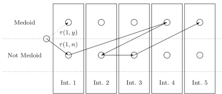
Fig. 2 An ant travelling through the construction graph. The pheromone values are stored in the edges: the order of visiting the data instances is random and thepheromone valuesrepresent the desirability of considering an instancexas a medoid (τ(x,y)value) or not (τ(x,n)value)
3.1 METACOC: a medoid set ACO clustering algorithm
The METACOC algorithm is based on several ants looking for the best path in the construction graph. The construction graph is composed by all data instances. Solutions are generated by choosing medoids (data instances) and assigning remaining data instances deterministically to them, according to their distance in relation to the selected medoids. The medoids selection
is illustrated in Fig.2. The rationale is that once the medoids are determined, there is a
deterministic optimal cluster allocation based on the similarity/dissimilarity values.
Each ant (a) has the following features:
– a list of visited data instances (tba);
– a set of chosen medoidsMa, which is initially empty.
Ants have two possible search strategies, exploitation and exploration. In each iteration,
an ant chooses the strategy for the medoid assignment j according to the pseudo-random
proportional rule (Dorigo and Gambardella 1997)
j =
argmaxu∈{y,n}{τ(i,u)}if q≤q0
S otherwise , (3)
where{y,n}are the possibilities (to be or not to be a medoid) to data instancei(see Fig.2),
τ(i,u)is the pheromone value betweeni(the data instance) andu(the condition “yes” or “no”
to become a medoid),q0is the user-defined exploitation probability,qis a random number
distributed uniformly in [0, 1] for strategy selection andS is the ACO-based exploration
strategy. The ACO-based exploration strategySis defined by
S=P(i,u)= τ(i,u)
l∈{y,n}τ(i,l)
, (4)
whereP(i,u)is the probability that data instancei could be selected as a medoid or not
andu∈ {y,n}. Note that METACOC does not use heuristic information to select a medoid.
While the number of selected medoidsmis less thank, wherekis the pre-defined number
of clusters, any data instance can be selected as a new medoid and the pheromone values are used to decide whether a data instance is considered a medoid or not. When the maximum number of medoids is reached, the selection process stops and the remaining data instances are set to not be medoids.
1. Initialize the pheromone matrixτ0.
2. Initialize each anta: set the chosen medoids Ma = ∅and the visited data instances
tba= ∅.
3. For each ant, check if all instances have been visited (|tba| ==n) or all medoids have
been chosen (|Ma| ==k). If not:
(a) select the next data instancei.
(b) choose a search strategy;
(c) ifiis selected as a medoid add it toMa;
(d) addito the list of visited data instancestba.
4. Assign each data instance to its closest medoid and calculate the objective function value
for each anta:
Ja= n i=1 |Ma| min j=1d(xi,m a j), (5)
wherexi represents a data instance andmjrepresents a medoid inMa.
5. Choose the best solution: (a) rank the ants solutions;
(b) if an ant has less medoids thankit is eliminated from the ranking;
(c) choose the best anta∗(iteration-best solution);
(d) comparea∗with the best-so-far solutiona∗∗and update this value with the maximum
between them.
6. Update the pheromone trails (global updating rule). Only therbest ants add pheromone:
τt+1(i,j)=(1−ρ)τt(i,j)+ r h=1 Δτt(i,j)h, Δτt(i,j)h = 1 Jh, (6)
whereρis the pheromone evaporation rate, (0< ρ <1),tis the iteration counter,ris
the number of elitist ants andJh is the quality of the solution created by anth.
7. Check termination condition:
(a) if the number of iterations is greater than the maximum number of iterations, it
finishes choosing the best-so-far solutiona∗∗;
(b) otherwise, go to step 2.
Once this process has finished, the best-so-far solution is chosen as the solution found by the algorithm. The solution consists of a set of medoids, which are the data instances represen-tative of the clusters. Each data instance is then assigned to its closest medoid to define the clusters.
In terms of computational complexity, we can assume that all data instances are visited
during the search process—although in practice this is not frequent—which takesO(An)
(where Ais the number of ants andnis the number of data instances). The algorithm also
includes a step that assigns each data instance to its closest medoid, which takesO(Ank)
(wherek is the number of medoids). The evaluation involves calculating the similarity of
each data instance to its assigned medoid, which takesO(An). Finally, the ranking of
solu-tions takes O(AlogA) and the pheromone update uses r elitist ants and visits all data
instances, which takes O(r n). Since these steps are repeated T iterations, the total
com-plexity isO(T An)+O(T Ank)+O(T AlogA)+O(T r n)—asO(T Ank)≥O(T An)≥
3.2 METACOC-K: a k-adaptive extension of METACOC
The proposed METACOC algorithm cannot choose the number of clusters, but requires as
input a value fork. This section presents the METACOC-K algorithm, which allows the
estimation of the number of clusters using METACOC as a starting point. The main features of METACOC-K are:
– each ant can have a different number of clusters;
– the quality metric is designed to balance between the number of clusters and the cluster assignment cost.
The first improvement is a straightforward modification of the ant behaviour, where each
ant chooses a random numberk of clusters to build a solution. The value ofk is limited
to a pre-defined range[kmin,kmax]. This is used to allow the algorithm to explore different
numbers of clusters. The second improvement consists in the solution evaluation, which now takes into account that each candidate solution can have a different number of clusters. As the metric used to update the pheromone information, we take the average silhouette calculated as
Avg_sil(X)=
x∈Xsil(x)
|X| , (7)
wherex ∈Xis a data instance and sil(x)is the silhouette metric (Kaufman and Rousseeuw
2009) given by sil(x)= d(x,Cclosest)− j∈Cxd(x,j) |Cx| max j∈Cxd(x,j) |Cx| ,d(x,Cclosest) , (8)
whered(x,j)is the distance between data instancesxand j,d(x,Cclosest)is the distance1
betweenxand the closest neighbouring clusterCclosest,Cxis the cluster to which elementx
belongs and|Cx|represents the number of elements ofCx. The silhouette compares tightness
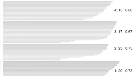
and separation of clusters. It is calculated by data instance and gives information about those data instances that are well assigned to a cluster and those that should be moved. The silhouette of all data instances provides an appreciation of the clusters’ quality (in a similar way of a Riemann integral). The area of the shape defined by silhouette is useful to determine the
quality of the number of clusters selection (see Fig.3).
The METACOC-K algorithm follows a structure similar to METACOC. The main differ-ences are:
1. Selection of the number of clusters:
(a) during the ant initialization (step 2 in METACOC), it additionally chooses uniformly
at random the number of clusters in the range[kmin,kmax]; the solution is then created
using the same procedure as in METACOC. 2. Solution evaluation:
(a) candidate solutions are evaluated using the average silhouette (Eq.7), which evaluates
the balance between the number of clusters and the cluster assignment cost (step 4 in METACOC).
Concerning the computational complexity of METACOC-K, we have to consider that the silhouette calculation is more expensive. The silhouette is used to evaluate the solutions,
1The distance between data instancexand a clusterCis the average of the distances betweenxand all data instances inC. The cluster with the lowest average distance is considered the closest neighbouring cluster.
75 74 68 61 72 63 73 64 62 66 71 69 65 67 70 44 48 47 46 45 53 58 60 51 49 59 56 52 50 55 57 54 41 43 42 40 38 39 37 21 30 29 24 36 31 34 22 23 33 35 28 25 27 32 26 7 17 20 5 1 19 15 18 4 13 16 2 14 3 12 8 11 9 6 10 Silhouette width si 1: 20 | 0.73 2: 23 | 0.75 3: 17 | 0.67 4: 15 | 0.80
Fig. 3 Silhouette for a dataset where four clusters have been discriminated:the first valuerepresents the cluster number,the secondis the number of instances andthe thirdis the average silhouette of the cluster
(cluster number:instances|silhouette). The average silhouette value across all clusters is 0.74, which measures
the quality of the number of clusters selection
and it involves the distance between every pair of data instancesnand the distance between
each data instance and thek medoids, repeated overT iterations; therefore, the evaluation
of solutions is O(T An2k)(where Ais the number of ants). Since the remaining steps are
similar to METACOC andO(T An2k)≥O(T Ank), the complexity remainsO(T An2k).
4 Computational experiments
This section presents the experiments that were carried out to measure the performance of the proposed algorithms: METACOC and METACOC-K. METACOC was compared against K-means, ACOC and PAM as non-adaptive algorithms (i.e. algorithms that required a fixed number of clusters), whereas METACOC-K was compared against EMBIC, Clues and PAMK as adaptive algorithms (i.e. algorithms that do not required a fixed number of clusters). 4.1 Datasets
We divided the computational results in three sets of experiments. In the first set of experi-ments, we evaluated the proposed algorithms on synthetic datasets. The following synthetic datasets were generated:
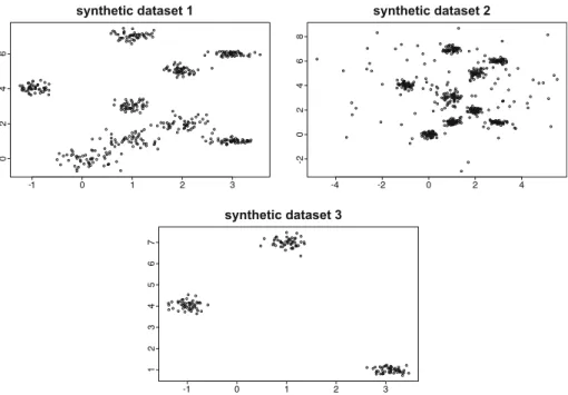
– synthetic dataset 1: This dataset corresponds to points in a two-dimensional Euclidean space, where nine clusters of points, each derived from a two-dimensional Gaussian distribution, were generated. There are three Gaussians which are closer than the rest.
This dataset has 450 instances, and it is illustrated in the top-left plot in Fig.4;
– synthetic dataset 2: This second dataset is generated analogously to dataset 1 (nine clus-ters of points), but with additional noisy data in the background. This dataset has 550
Fig. 4 Data points generated by the three synthetic datasets that have been used for the experiments: the first
(top-left plot) shows nine two-dimensional Gaussian distributions, where three of them are very close; the
second (top-right plot) introduces noise to the nine Gaussian models; and the last one (bottom-centre plot) shows three well-separated Gaussian models
– synthetic dataset 3: This dataset is composed of three two-dimensional Gaussian distri-butions, which are well separated. This dataset has 150 instances, and it is illustrated in
the bottom-centre plot in Fig.4.
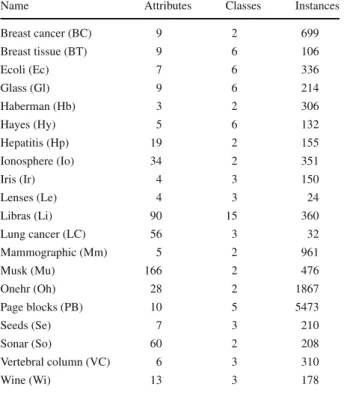
In the second set of experiments, we chose 20 real-world datasets from the UCI Machine Learning Repository (Frank and Asuncion 2010). These datasets are benchmark datasets
for clustering and classification tasks. Table1shows the main characteristics for each UCI
dataset used in our experiments. Finally, in the third set of experiments, we chose 10 time series benchmark datasets from the UCR time series repository (Chen et al. 2015) in order to evaluate the medoid-based methodologies in a specific area where they have been successful.
Table2shows the main characteristics for each UCR dataset used in our experiments.
4.2 Experimental setup
This section briefly describes the selected algorithms used for comparison. ACOC (Kao and Cheng 2006) is an ACO clustering algorithm based on centroids. ACOC uses a pheromone matrix to store the relationship between the data instances and the centroid labels, where ants assign each data instance to one of the available clusters and cluster centroids are adjusted based on this assignment. Comparing ACOC to METACOC and METACOC-K, both META-COC and METAMETA-COC-K use a different construction graph, where an ant chooses whether an instance is a medoid or not (i.e. it is always a binary decision regardless of the number of clusters).
K-means (MacQueen 1967) is an iterative algorithm based on centroids, which are ran-domly selected at the beginning. The goal of the algorithm is to find the best centroid positions.
Table 1 Description of the UCI datasets used in the experiments
The table shows the number of numerical attributes, classes and data instances per dataset
Name Attributes Classes Instances
Breast cancer (BC) 9 2 699 Breast tissue (BT) 9 6 106 Ecoli (Ec) 7 6 336 Glass (Gl) 9 6 214 Haberman (Hb) 3 2 306 Hayes (Hy) 5 6 132 Hepatitis (Hp) 19 2 155 Ionosphere (Io) 34 2 351 Iris (Ir) 4 3 150 Lenses (Le) 4 3 24 Libras (Li) 90 15 360 Lung cancer (LC) 56 3 32 Mammographic (Mm) 5 2 961 Musk (Mu) 166 2 476 Onehr (Oh) 28 2 1867 Page blocks (PB) 10 5 5473 Seeds (Se) 7 3 210 Sonar (So) 60 2 208 Vertebral column (VC) 6 3 310 Wine (Wi) 13 3 178
Table 2 Description of the UCR datasets used in the experiments
The table shows the number of numerical attributes, classes and data instances per dataset
Name Attributes Classes Instances
ArrowHead (AH) 251 3 211 BirdChicken (BC) 512 2 40 CBF (CB) 128 3 930 Coffee (Co) 286 2 56 ECGFive (EF) 136 2 884 Ham (Ha) 431 2 214 Herring (He) 512 2 128 ItalyPowerDemand (IP) 24 2 1106 Lighting2 (Lt) 637 2 121 SonyAIBORobot (SA) 70 2 621
It is executed in two steps: in the first step, it assigns the data to the closest centroid (cluster); in the second step, it calculates the new position of each centroid as the centroid of the data that have been assigned to it.
PAM (Kaufman and Rousseeuw 1987) is similar to K-means, but it uses medoids instead of centroids. PAM can work with a dissimilarity/similarity matrix, which is used to calculate the overall cost of a cluster. PAMK (Kaufman and Rousseeuw 2009) is an extension of PAM, which calculates the number of clusters using the silhouette as a decision metric.
EMBIC (Fraley and Raftery 2007) combines EM with the Bayesian information criterion (BIC). The EM algorithm tries to optimize the parameters of an estimator (in this case, Gaussian Mixture Models), and BIC adds a penalty to the likelihood based on the number of parameters. This is helpful when the number of clusters needs to be controlled. Finally, Clues (Wang et al. 2007) creates a cluster per data instance and merges the clusters according to the silhouette metric.
We used the R standard implementation2of K-means, PAM, PAMK, EMBIC and Clues:
for each algorithm, the number of iterations was set to 100 and the remaining parameters were used with their default values; the initial centroids for K-means were randomly chosen. The parameters of ACOC, METACOC and METACOC-K algorithms have been set in a similar way as in the original work (Kao and Cheng 2006): the number on ants is 1000, the number
of elitist ants is 10, the exploitation probability (q0) is 0.0001, the initial pheromone values
follow a uniform distribution in[0.7,0.8],β=2.0 (only used by ACOC),ρ=0.1 and the
maximum number of iterations is 1000.
All the experiments have been carried out using the Euclidean distance as the basic per-formance metric, which is defined as
d(xi,xj)= ||xi−xj|| =
v
(xiv−xvj)2, (9)
wherexi,xjrepresent two data instances andvrepresents each attribute of the data instance.
Additionally, K-means, PAM, ACOC and METACOC algorithms need the number of clusters as an initial parameter. The experiments have been carried out 100 times per algorithm and dataset used, and the average is reported.
The evaluation of the experiments has been focused on two different criteria: on one hand, the synthetic datasets have been evaluated according to the cluster discrimination and the performance of the algorithm to discriminate the original clusters in the noisy case; on the other hand, the real-world datasets have been evaluated using the silhouette metric, which is optimized directly by the PAMK, EMBIC, Clues and METACOC-K algorithms, and indirectly by the remaining algorithms (K-means, PAM, ACOC and METACOC) when they optimize the cost function defined by the Euclidean metric.
4.3 Synthetic experiments
This section presents the result for the synthetic experiments. We have measured how the algorithms discriminate data, applying the adjusted rand index metric (Hubert and Ara-bie 1985) to the solutions generated for each dataset. As mentioned above, we considered
three datasets. Table3shows the average results for each algorithm (average±SD) over
100 executions; no standard deviation is shown when its value is lower than 0.001. For the adaptive algorithms METACOC-K, PAMK, EMBIC and Clues, the average number
of clusters identified is in brackets. Table4shows the median results for each algorithm.
Finally, Table5shows the best results obtained by each algorithm: a value in this table
cor-responds to the highest value in terms of the adjusted rand index metric achieved by an algorithm.
Table3shows that METACOC is the algorithm that is able to clearly discriminate the
data in all three datasets, achieving the highest average adjusted rand index of all algorithms. METACOC-K also performs well overall, although it seems to have more problems discrim-inating the cluster boundaries on the synthetic dataset 1. PAM and PAMK obtain similar
Table 3 Average results of the application of the algorithms to the synthetic datasets in adjusted rand index terms, calculated over 100 executions (average±SD); no SD is shown for an algorithm when all values are lower than 0.001
K-means ACOC PAM METACOC
Synthetic 1 0.812±0.088 0.922±0.017 0.975 0.992±0.002 Synthetic 2 0.783±0.080 0.892±0.030 0.955 0.963±0.005 Synthetic 3 0.812±0.237 1.0±0.000 1.0 1.0±0.000
EMBIC Clues PAMK METACOC-K
Synthetic 1 0.985 (9) 0.892 (15) 0.975 (9) 0.967±0.041 (9) Synthetic 2 0.667 (9) 0.959 (9) 0.928 (10) 0.954±0.011 (9) Synthetic 3 1.0(3) 0.293 (12) 1.0(3) 1.0±0.000 (3) The best result for a given dataset is shown in boldface; for adaptive algorithms, the average number of clusters identified is in brackets
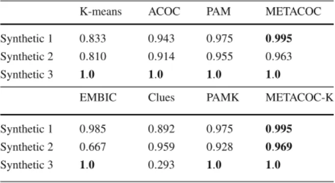
Table 4 Median value for the adjusted rand index on the synthetic datasets
Each value corresponds to the median value achieved by an algorithm over 100 executions. The best result for a given dataset is shown in boldface
K-means ACOC PAM METACOC
Synthetic 1 0.833 0.943 0.975 0.995
Synthetic 2 0.810 0.914 0.955 0.963 Synthetic 3 1.0 1.0 1.0 1.0
EMBIC Clues PAMK METACOC-K
Synthetic 1 0.985 0.892 0.975 0.995
Synthetic 2 0.667 0.959 0.928 0.969
Synthetic 3 1.0 0.293 1.0 1.0
performances, but PAMK has problems in identifying the correct number of clusters on syn-thetic dataset 2. This is also the case for EMBIC, which performs well on synsyn-thetic dataset 1 and synthetic dataset 3, but has problems on synthetic dataset 2. Clues is the algorithm that achieved the lowest average in synthetic dataset 3, since it generates several clusters—many more than the existing clusters in the data—during the discrimination process (12 cluster); it achieves a good performance in the remaining datasets. ACOC performs well overall, with the exception of synthetic dataset 2, where it has problems discriminating the cluster centres. K-means has problems in all three datasets: while it managed to discriminate the clusters in the majority of the runs, it seems to be more sensitive to the initial centroids’ positions, as can be noticed by its lower average and higher standard deviation values.
Looking closely at the median (Table4) and average (Table3) results, we get an intuition about the convergence of METACOC and METACOC-K. METACOC has similar values for both median and average, showing that the solutions are similar over multiple runs. METACOC-K variates more according to the average, which is usually lower than the median. This shows that an outlier result might appear when we apply METACOC-K multiple times, which affects the average value. Comparing the median of METACOC-K with the maximum
Table 5 Highest value for the adjusted rand index on the synthetic datasets
Each value corresponds to the highest value achieved by an algorithm over 100 executions. The best result for a given dataset is shown in boldface
K-means ACOC PAM METACOC
Synthetic 1 0.995 0.995 0.975 1.0
Synthetic 2 0.955 0.947 0.955 0.972
Synthetic 3 1.0 1.0 1.0 1.0
EMBIC Clues PAMK METACOC-K
Synthetic 1 0.985 0.892 0.975 1.0
Synthetic 2 0.667 0.959 0.928 0.972
Synthetic 3 1.0 0.293 1.0 1.0
which suggests that in more than 50 % of the runs METACOC-K obtains a better or similar result than the best result of the other algorithms.
These results show that the proposed algorithms are able to find good results when com-pared with classical algorithms using synthetic datasets and in general achieved better results than ACOC.
4.4 Experiments with real-world datasets
This section presents the results of the experiments with real-world datasets. In this case, the evaluation is focused on the algorithms objectives—i.e. optimizing the silhouette metric.
Table6shows the results of all the non-adaptive algorithms, and Table7shows the results of
the adaptive algorithms. The values in these tables represent the average and standard
devi-ation (average±SD) over 100 executions; no standard deviation is shown for an algorithm
when all values are lower than 0.001 (EMBIC, Clues and PAMK results).
We have performed a statistical analysis using the Wilcoxon test (Demšar 2006). We
compared the performance of METACOC against PAM (Table6) and METACOC-K against
PAMK (Table7): the datasets where METACOC (METACOC-K)’s performance is statisti-cally significantly better according to the Wilcoxon test with a significant level of 0.05 are marked with the symbol ; the datasets where METACOC (METACOC-K)’s performance is statistically significantly worse are marked with the symbol ; if no symbol is shown, no significant difference was observed. In the first case, METACOC and PAM have been cho-sen since both are medoid-based clustering algorithms, but METACOC employs a different search strategy compared to PAM. In the second case, METACOC-K and PAMK have been chosen as PAMK is the adaptive algorithm with the best performance among the algorithms optimizing the silhouette metric.
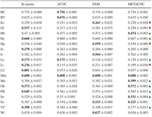
Table6shows that METACOC obtains statistically significantly better results than PAM
in 8 out of 20 datasets, while achieving statistically significantly worse results in only 3. The comparison of METACOC with the rest of the non-adaptive algorithms shows that the algorithm achieves the best results in 6 out of 20 datasets, a similar results obtained by PAM while K-means obtains the best results in 10 out of 20 datasets. The good performance of K-means is likely a consequence that this algorithm is able to move its centroids in the whole search space (i.e. centroid values do not necessarily correspond to values from a data instance), while METACOC and PAM—the medoid-based algorithms—choose data instances as medoids, which probably reduces the silhouette values. This case is similar when ACOC and METACOC are compared: the ACOC algorithm is able to use the whole search space, while METACOC has to use a reduced and discrete version based only on the data instances. As a consequence, the performance of ACOC and METACOC is similar in
Table 6 Average results of the application of the non-adaptive algorithms to the UCI datasets in silhouette metric terms (average±SD)
K-means ACOC PAM METACOC
BC 0.755±0.000 0.756±0.001 0.754±0.000 0.754±0.001 BT 0.625±0.014 0.676±0.060 0.633±0.009 0.635±0.050 Ec 0.259±0.038 0.231±0.032 0.263±0.022 0.230±0.028 Gl 0.537±0.115 0.317±0.132 0.281±0.075 0.250±0.091 Hb 0.47±0.003 0.471±0.002 0.472±0.000 0.474±0.003 Hy 0.668±0.000 0.668±0.001 0.665±0.000 0.667±0.001 Hp 0.536±0.049 0.549±0.003 0.559±0.015 0.550±0.009 Io 0.270±0.000 0.263±0.004 0.266±0.000 0.265±0.008 Ir 0.562±0.013 0.562±0.004 0.564±0.007 0.562±0.005 Le 0.175±0.033 0.175±0.011 0.124±0.012 0.129±0.031 Li 0.236±0.017 0.115±0.035 0.211±0.007 0.199±0.030 LC 0.081±0.014 0.073±0.020 0.041±0.010 0.037±0.000 Mm 0.608±0.002 0.608±0.001 0.608±0.001 0.608±0.002 Mu 0.394±0.037 0.393±0.012 0.382±0.021 0.399±0.022 Oh 0.372±0.002 0.365±0.026 0.361±0.000 0.372±0.003 PB 0.649±0.030 0.561±0.035 0.551±0.015 0.565±0.021 Se 0.529±0.024 0.53±0.001 0.524±0.008 0.531±0.004 So 0.187±0.000 0.194±0.006 0.215±0.000 0.215±0.001 VC 0.398±0.021 0.382±0.006 0.348±0.011 0.377±0.013 Wi 0.629±0.004 0.636±0.002 0.637±0.002 0.636±0.003 The performance of METACOC is statistically significantly better than PAM according to the Wilcoxon test with a significance level of 0.05 in the datasets marked with the symbol ; the performance of METACOC is statistically significantly worse than PAM in the datasets marked with the symbol ; if no symbol is shown, no significant difference was observed. The best result for a given dataset is shown in boldface
several cases. However, it is important to remark that centroid-based algorithms cannot be used when only the distances/similarities among data are known.
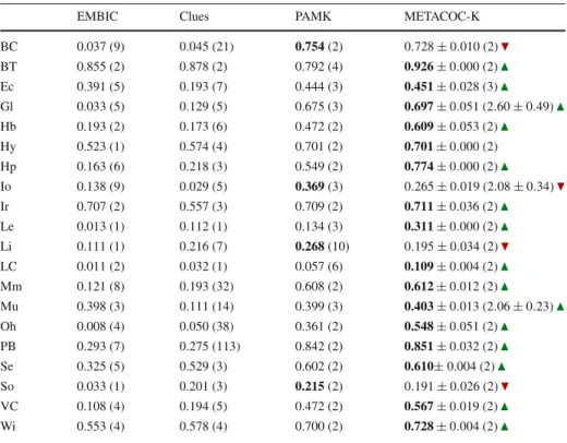
Table7 shows the experimental results for the datasets when the adaptive algorithms
are considered. This table shows that METACOC-K obtains statistically significantly better results than PAMK in 15 of the 20 datasets, while achieving statistically significantly worse results in only 4. When METACOC-K is compared with the rest of the adaptive algorithms, it obtains better results than both EMBIC and Clues—with the exception of the So and Li datasets, where Clues obtains better results.
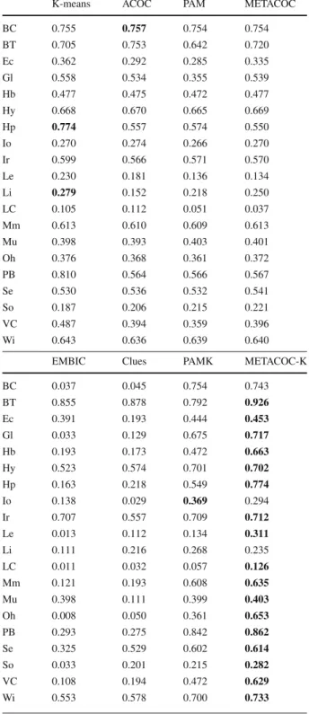
Table8presents a summary of the best results obtained by each algorithm. A value in the
table corresponds to the highest value in terms of the silhouette metric achieved by an algo-rithm over 100 executions. These results show again the better performance of METACOC-K in optimizing the silhouette metric over the remaining algorithms: METACOC-K obtained the highest value in 17 of the 20 datasets; although K-means optimizes the silhouette metric only indirectly by minimizing the Euclidean error in the clusters, it obtained the highest value in two datasets (in one of them it tied with METACOC-K); ACOC and PAMK obtained the highest value in one dataset each.
We also compared the best results of K-means against a single run of METACOC and METACOC-K. This comparison presents a balance between the computational time and
Table 7 Average results of the application of the adaptive algorithms to the UCI datasets in silhouette metric terms (average±SD); no standard deviation is shown for an algorithm when all values are lower than 0.001
EMBIC Clues PAMK METACOC-K
BC 0.037 (9) 0.045 (21) 0.754(2) 0.728±0.010 (2) BT 0.855 (2) 0.878 (2) 0.792 (4) 0.926±0.000 (2) Ec 0.391 (5) 0.193 (7) 0.444 (3) 0.451±0.028 (3) Gl 0.033 (5) 0.129 (5) 0.675 (3) 0.697±0.051 (2.60±0.49) Hb 0.193 (2) 0.173 (6) 0.472 (2) 0.609±0.053 (2) Hy 0.523 (1) 0.574 (4) 0.701 (2) 0.701±0.000 (2) Hp 0.163 (6) 0.218 (3) 0.549 (2) 0.774±0.000 (2) Io 0.138 (9) 0.029 (5) 0.369(3) 0.265±0.019 (2.08±0.34) Ir 0.707 (2) 0.557 (3) 0.709 (2) 0.711±0.036 (2) Le 0.013 (1) 0.112 (1) 0.134 (3) 0.311±0.000 (2) Li 0.111 (1) 0.216 (7) 0.268(10) 0.195±0.034 (2) LC 0.011 (2) 0.032 (1) 0.057 (6) 0.109±0.004 (2) Mm 0.121 (8) 0.193 (32) 0.608 (2) 0.612±0.012 (2) Mu 0.398 (3) 0.111 (14) 0.399 (3) 0.403±0.013 (2.06±0.23) Oh 0.008 (4) 0.050 (38) 0.361 (2) 0.548±0.051 (2) PB 0.293 (7) 0.275 (113) 0.842 (2) 0.851±0.032 (2) Se 0.325 (5) 0.529 (3) 0.602 (2) 0.610±0.004 (2) So 0.033 (1) 0.201 (3) 0.215(2) 0.191±0.026 (2) VC 0.108 (4) 0.194 (5) 0.472 (2) 0.567±0.019 (2) Wi 0.553 (4) 0.578 (4) 0.700 (2) 0.728±0.004 (2)
The performance of METACOC-K is statistically significantly better than PAMK according to Wilcoxon test with significance level of 0.05 in the datasets marked with the symbol ; the performance of METACOC-K is statistically significantly worse than PAMK in the datasets marked with the symbol ; if no symbol is shown, no significant difference was observed. The best result for a given dataset is shown in boldface; the average number of clusters identified is in brackets
the performance of the algorithms, given that the proposed algorithms use a more time-consuming ACO procedure where multiple candidate solutions are evaluated, while K-means
employs a faster local search strategy. The results are presented in Table9. A value in the table
corresponds to the average of the best K-means value over 30 executions (where the best value is determined over 30 restarts for each execution) and a single execution of METACOC and METACOC-K. The results show that METACOC-K is the best of the ACO-based algorithms, achieving statistically significantly better results than K-means in 14 of the 20 datasets and statistically significantly worse results in only one dataset; in the remaining 5 datasets, no statistically significant differences were detected. In this case is evident the advantage of the ACO procedure, since it leads to the creation of high quality solutions. The results obtained by METACOC are mixed: K-means is statistically significantly better than METACOC in 9; K-means is statistically significantly worse than METACOC in 5 datasets; and they have similar performances in 4 datasets. Given the stochastic nature of the ACO search, better results might be obtained by multiple executions of METACOC, at the cost of a higher computational time.
Overall, we consider the results presented in Tables6,7,8and9positive. In summary,
pro-Table 8 Highest value for the silhouette metric on the UCI datasets
Each value corresponds to the highest value achieved by an algorithm over 100 executions. The best result for a given dataset is shown in boldface
K-means ACOC PAM METACOC
BC 0.755 0.757 0.754 0.754 BT 0.705 0.753 0.642 0.720 Ec 0.362 0.292 0.285 0.335 Gl 0.558 0.534 0.355 0.539 Hb 0.477 0.475 0.472 0.477 Hy 0.668 0.670 0.665 0.669 Hp 0.774 0.557 0.574 0.550 Io 0.270 0.274 0.266 0.270 Ir 0.599 0.566 0.571 0.570 Le 0.230 0.181 0.136 0.134 Li 0.279 0.152 0.218 0.250 LC 0.105 0.112 0.051 0.037 Mm 0.613 0.610 0.609 0.613 Mu 0.398 0.393 0.403 0.401 Oh 0.376 0.368 0.361 0.372 PB 0.810 0.564 0.566 0.567 Se 0.530 0.536 0.532 0.541 So 0.187 0.206 0.215 0.221 VC 0.487 0.394 0.359 0.396 Wi 0.643 0.636 0.639 0.640
EMBIC Clues PAMK METACOC-K
BC 0.037 0.045 0.754 0.743 BT 0.855 0.878 0.792 0.926 Ec 0.391 0.193 0.444 0.453 Gl 0.033 0.129 0.675 0.717 Hb 0.193 0.173 0.472 0.663 Hy 0.523 0.574 0.701 0.702 Hp 0.163 0.218 0.549 0.774 Io 0.138 0.029 0.369 0.294 Ir 0.707 0.557 0.709 0.712 Le 0.013 0.112 0.134 0.311 Li 0.111 0.216 0.268 0.235 LC 0.011 0.032 0.057 0.126 Mm 0.121 0.193 0.608 0.635 Mu 0.398 0.111 0.399 0.403 Oh 0.008 0.050 0.361 0.653 PB 0.293 0.275 0.842 0.862 Se 0.325 0.529 0.602 0.614 So 0.033 0.201 0.215 0.282 VC 0.108 0.194 0.472 0.629 Wi 0.553 0.578 0.700 0.733
Table 9 Average results of the best K-means run computed over 30 restarts, and a single run of METACOC and METACOC-K on the UCI datasets in silhouette metric terms (average±SD)
The performance of METACOC and METACOC-K is statistically significantly better than K-means according to Wilcoxon test with significance level of 0.05 in the datasets marked with the symbol
; the performance of
METACOC and METACOC-K is statistically significantly worse than K-means in the datasets marked with the symbol ; if no symbol is shown, no significant difference was observed. The best result for a given dataset is shown in boldface
K-means METACOC METACOC-K
BC 0.755±0.000 0.758±0.002 0.728±0.010 BT 0.635±0.004 0.639±0.051 0.926±0.000 Ec 0.303±0.007 0.227±0.022 0.451±0.028 Gl 0.541±0.002 0.286±0.083 0.697±0.051 Hb 0.477±0.003 0.488±0.002 0.609±0.053 Hy 0.668±0.000 0.669±0.002 0.701±0.000 Hp 0.676±0.007 0.540±0.005 0.774±0.000 Io 0.270±0.000 0.271±0.003 0.265±0.019 Ir 0.577±0.004 0.557±0.004 0.711±0.036 Le 0.200±0.002 0.117±0.027 0.311±0.000 Li 0.243±0.001 0.194±0.028 0.195±0.034 LC 0.095±0.011 0.047±0.000 0.109±0.004 Mm 0.613±0.001 0.618±0.003 0.612±0.012 Mu 0.398±0.002 0.401±0.020 0.403±0.013 Oh 0.376±0.002 0.379±0.006 0.548±0.051 PB 0.751±0.008 0.575±0.017 0.851±0.032 Se 0.530±0.003 0.541±0.009 0.610±0.004 So 0.187±0.000 0.215±0.001 0.191±0.026 VC 0.417±0.007 0.367±0.017 0.567±0.019 Wi 0.634±0.002 0.646±0.009 0.728±0.004
posed algorithm that can adapt the number of clusters, obtains the highest results of all the algorithms in 17 of the 20 datasets. More importantly, it statistically significantly outperforms PAMK in 15 of the 20 datasets.
4.5 Time series experiments
In this section, we present a set of experiments focused on a specific domain where medoid-based approaches have been successful: time series analysis (Liao 2005). We have selected ten datasets from the UCR Time Series Classification Archive (Chen et al. 2015). Details of these datasets are presented in Table2. The similarity matrix derived from the alignment between two time series is generated applying the Dynamic Time Wrapping distance (Keogh and Ratanamahatana 2005). Table10shows the experimental results for the medoid-based algorithms: PAM, METACOC, Clues, PAMK and METACOC-K. The values in this table
represent the average and standard deviation (average±SD) over 100 executions; no standard
deviation is shown for an algorithm when all values are lower than 0.001 (Clues and PAMK results).
In these experiments, we use PAM, Clues and PAMK as benchmark for the Wilcoxon test with significance level of 0.05, comparing them with METACOC and METACOC-K, respectively. METACOC shows better performance compared with PAM overall, achieving statistically significantly better results in two datasets (CB and SA) and statistically signifi-cantly worse results in only one dataset (Lt). METACOC-K achieved statistically signifisignifi-cantly better results than Clues in 9 out of 10 datasets and no statistically significant differences were detected in only one dataset (He); compared with PAMK, METACOC-K achieved sta-tistically significantly better results in 6 out of 10 datasets (AH, CB, Co, Ha, IP and SA) and
Table 10 Average results of the application of the adaptive algorithms to the UCR time series datasets in silhouette metric terms (average±SD); no SD is shown for an algorithm when all values are lower than 0.001
The performance of PAM (Clues and PAMK) is statistically significantly better than METACOC (METACOC-K) according to Wilcoxon test with significance level of 0.05 in the datasets marked with the symbol
; the performance of PAM (Clues and PAMK) is statistically significantly worse than METACOC (METACOC-K) in the datasets marked with the symbol ; if no symbol is shown, no significant difference was observed. The best result for a given dataset is shown in boldface; the average number of clusters identified by Clues, PAMK and METACOC-K is shown in brackets PAM METACOC AH 21.88±0.010 22.20±0.018 BC 34.10±0.000 34.10±0.000 CB 13.56±0.025 14.55±0.018 Co 28.78±0.013 28.78±0.000 EF 40.31±0.001 40.30±0.002 Ha 10.98±0.012 10.33±0.012 He 32.44±0.022 32.66±0.004 IP 63.08±0.044 63.25±0.003 Lt 21.06±0.027 15.02±0.024 SA 7.80±0.021 10.54±0.039
Clues PAMK METACOC-K
AH 11.53 (5) 46.99 (2) 74.58±0.025 (2) BC 0 (1) 35.57 (8) 35.58±0.012 (2) CB 8.51 (19) 23.74 (2) 27.51±0.007 (3) Co 0 (1) 28.78 (2) 32.03±0.047 (2) EF 20.91 (20) 40.31 (2) 40.40±0.007 (2) Ha 6.57 (4) 10.98 (2) 25.81±0.065 (2) He 33.05(2) 32.84 (2) 32.16±0.007 (2) IP 14.32 (24) 63.08 (2) 64.14±0.002 (2) Lt 9.73 (3) 21.06 (2) 21.37±0.017 (2) SA 6.16 (13) 15.83 (4) 16.56±0.062 (2)
no statistically significant differences were detected in the remaining datasets. Additionally, METACOC-K identified the right number of clusters in all cases but the AH dataset, which was also not identified by any of the adaptive algorithms.
4.6 Computational time
Table11shows the average computational time (average±SD) in seconds taken by
META-COC and METAMETA-COC-K on the UCI datasets over a fixed number of iterations. The algorithms are around 10 times slower than K-means, 6 times slower than PAM and Clues, 4 times slower than PAMK and similar to EMBIC. Overall, METACOC is faster than METACOC-K. We were expecting a higher computational time for METACOC-K, since the algorithm explores
solutions with different values fork and it uses a more complex evaluation function. In
our observations, both METACOC and METACOC-K are generally faster than ACOC. We attribute this to the simplified construction process compared to ACOC. As soon as the
algo-rithm selectskmedoids (wherekis the number of clusters), the solution construction process
stops, while ACOC must visit all instances of the dataset to create a solution.
Figure5illustrates the convergence of METACOC and METACOC-K. It is interesting to
note that METACOC-K converges faster than METACOC, while being slower than META-COC over the same number of iterations. This suggests that the computational time of METACOC-K can be improved by using a smaller number of iterations to reduce its overall computation time, without negative impact on its performance.
Table 11 Average computational time
(average±SD) in seconds taken by METACOC and
METACOC-K on the UCI datasets
The lowest value for a given dataset is shown in boldface
METACOC METACOC-K BC 10.11±0.042 17.52±0.073 BT 1.41±0.001 1.95±0.010 Ec 4.88±0.018 11.37±0.042 Gl 2.33±0.005 2.89±0.015 Hb 4.20±0.012 9.31±0.033 Hy 1.87±0.001 1.99±0.004 Hp 1.92±0.001 3.01±0.006 Io 5.06±0.008 12.27±0.062 Ir 2.11±0.003 2.31±0.007 Le 0.31±0.000 0.45±0.000 Li 3.98±0.009 8.81±0.031 LC 0.40±0.000 0.51±0.000 Mm 21.20±0.029 20.40±0.068 Mu 8.53±0.011 18.20±0.082 Oh 21.70±0.029 49.10±0.101 PB 45.10±0.081 100.40±0.192 Se 1.95±0.002 3.33±0.005 So 2.55±0.003 2.72±0.003 VC 5.22±0.009 7.89±0.026 Wi 2.33±0.001 2.51±0.005
5 Conclusions and future work
In this paper, we proposed two medoid-based ACO clustering algorithms, METACOC and METACOC-K. Medoid-based clustering algorithms only need the distances/similarities among data to find a solution and they are more robust to outliers. One of the main advantages of medoid-based algorithms is that they can directly be applied to problems where the fea-tures of data cannot be easily represented in a multi-dimensional space. The first algorithm, called METACOC, uses an ACO procedure to determine an optimal medoid set (METACOC algorithm). The second algorithm, called METACOC-K, uses an automatic selection of the number of clusters, useful for problems where the number of cluster is not known a priori.
We compared the proposed algorithms against classical clustering algorithms, both centroid- and medoid-based, in synthetic and real-world datasets. METACOC results were positive, statistically significantly outperforming PAM in 8 out of 20 real-world datasets and achieving competitive results against (centroid-based) K-means and ACOC algorithms, while using only the information about the distance among the data instances. METACOC-K results were also positive: it statistically significantly outperformed PAMK in 15 out of the 20 real-world datasets. METACOC-K was also the algorithm that consistently achieved the best results in the real-world datasets in the experiments optimizing the silhouette metric. Concerning the time series datasets, METACOC shows better performance compared with PAM overall, achieving statistically significantly better results in two datasets and statis-tically significantly worse results in only one dataset; METACOC-K achieved statisstatis-tically significantly better results than Clues in 9 out of 10 datasets and than PAMK in 6 out of 10 datasets, with no statistically significant differences detected in the remaining datasets.
Fig. 5 Illustration of the convergence of METACOC and METACOC-K on the breast cancer, breast tissue, Haberman and Wine UCI datasets
There are several future research directions. Both METACOC and METACOC-K do not employ heuristic information during the construction process—it would be interesting to investigate whether the search can be further improved by such information. Exploring the use of different cluster evaluation measures to improve the number of clusters selection in METACOC-K is also another interesting research direction—this can be evaluated in an automatic configuration setting (López-Ibáñez et al. 2011). At the moment, the selection of the number of clusters is not part of the construction graph, and therefore, it is not influenced by pheromone values—adding the selection to the construction graph might improve the search. Finally, the application of the algorithms in large-scale data analysis tasks is also a research direction worth further exploration.
Acknowledgments The authors would like to thank the anonymous reviewers and the associate editor for their valuable comments and suggestions. This work is supported by the Spanish Ministry of Sci-ence and Education under Project Code TIN2014-56494-C4-4-P, Comunidad Autonoma de Madrid under project CIBERDINE S2013/ICE-3095, United Kingdom government by the EPSRC project SeMaMatch EP/K032623/1 and Savier—an Airbus Defence & Space project (FUAM-076914 and FUAM-076915).
Open Access This article is distributed under the terms of the Creative Commons Attribution 4.0 Interna-tional License (http://creativecommons.org/licenses/by/4.0/), which permits unrestricted use, distribution, and reproduction in any medium, provided you give appropriate credit to the original author(s) and the source, provide a link to the Creative Commons license, and indicate if changes were made.
References
Ashok, L., & Messinger, D. W. (2012). A spectral image clustering algorithm based on ant colony optimization.
InProceedings of Algorithms and Technologies for Multispectral, Hyperspectral, and Ultraspectral
Imagery XVIII (SPIE 8390)(pp. 1–10). International Society for Optics and Photonics.
Cao, L. (2010). Domain-driven data mining: Challenges and prospects.IEEE Transactions on Knowledge and
Data Engineering,22(6), 755–769.
Chen, Y., Keogh, E., Hu, B., Begum, N., Bagnall, A., Mueen, A., & Batista, G. (2015). The UCR time series classification archive.www.cs.ucr.edu/~eamonn/time_series_data/.
Dempster, A. P., Laird, N. M., & Rubin, D. B. (1977). Maximum likelihood from incomplete data via the EM algorithm.Journal of the Royal Statistical Society, Series B (Methodological),39(1), 1–38.
Demšar, J. (2006). Statistical comparisons of classifiers over multiple data sets.Machine Learning Research,
7, 1–30.
Dorigo, M., & Gambardella, L. (1997). Ant colony system: A cooperative learning approach to the traveling salesman problem.IEEE Transactions on Evolutionary Computation,1(1), 53–66.
Dorigo, M., & Stützle, T. (2004).Ant colony optimization. Cambridge, MA: MIT Press.
Fernandes, C., Mora, A., Merelo, J., Ramos, V., Laredo, J., & Rosa, A. (2008). KANTS: Artifical ant system for classification. In M. Dorigo, M. Birattari, C. Blum, M. Clerc, T. Stützle, & A. Winfield (Eds.)Ant
Colony Optimization and Swarm Intelligence: 6th International Conference (ANTS 2008), LNCS(vol.
5217, pp. 339–346). Springer.
Fraley, C., & Raftery, A. E. (2007). Bayesian regularization for normal mixture estimation and model-based clustering.Journal of Classification,24(2), 155–181.
França, F., Coelho, G., & Zuben, F. (2008). bicACO: An ant colony inspired biclustering algorithm. In M. Dorigo, M. Birattari, C. Blum, M. Clerc, T. Stützle, & A. Winfield (Eds.),Ant colony optimization and
swarm intelligence, LNCS(Vol. 5217, pp. 401–402). Berlin, Heidelberg: Springer.
Frank, A., & Asuncion, A. (2010). UCI machine learning repository.http://archive.ics.uci.edu/ml. Hamdi, A., Antoine, V., Monmarché, N., Alimi, A., & Slimane, M. (2010). Artificial ants for automatic
clas-sification. In N. Monmarché, F. Guinand, & P. Siarry (Eds.),Artificial ants: From collective intelligence
to real life optimization and beyond, Chapter 13(pp. 265–290). London: ISTE-Wiley.
Handl, J., Knowles, J., & Dorigo, M. (2006). Ant-based clustering and topographic mapping.Artificial Life,
12(1), 35–62.
Herrmann, L., & Ultsch, A. (2008) The architecture of ant-based clustering to improve topographic mapping. In M. Dorigo, M. Birattari, C. Blum, M. Clerc, T. Stützle, & A. Winfield (Eds.)Ant colony optimization
and swarm intelligence: 6th international conference (ANTS 2008), LNCS(vol. 5217, pp. 379–386).
Springer.
Hruschka, E., Campello, R., Freitas, A., & de Carvalho, A. (2009). A survey of evolutionary algorithms for clustering.IEEE Transactions on Systems, Man, and Cybernetics, Part C: Applications and Reviews,
39(2), 133–155.
Hubert, L., & Arabie, P. (1985). Comparing partitions.Journal of Classification,2(1), 193–218.
Jafar, O. M., & Sivakumar, R. (2010). Ant-based clustering algorithms: A brief survey.International Journal
of Computer Theory and Engineering,2(5), 787–796.
Kao, Y., & Cheng, K. (2006) An ACO-based clustering algorithm. In M. Dorigo, L. Gambardella, M. Birat-tari, A. Martinoli, R. Poli, & T. Stützle (Eds.)Ant colony optimization and swarm intelligence: 5th
international conference (ANTS 2006), LNCS(vol. 4150, pp. 340–347). Springer.
Kaufman, L., & Rousseeuw, P. (1987).Clustering by means of medoids. No. 87 in Reports of the Faculty of Mathematics and Informatics. Delft University of Technology.
Kaufman, L., & Rousseeuw, P. J. (2009).Finding groups in data: An introduction to cluster analysis(Vol. 344). New Jersey: Wiley.
Keogh, E., & Ratanamahatana, C. A. (2005). Exact indexing of dynamic time warping.Knowledge and
Information Systems,7(3), 358–386.
Larose, D. T. (2005).Discovering knowledge in data. New Jersey: Wiley.
López-Ibáñez, M., Dubois-Lacoste, J., Stützle, T., & Birattari, M. (2011).The irace package: Iterated racing
for automatic algorithm configuration. Technical Report No. TR/IRIDIA/2011-004, IRIDIA, Université
Libre de Bruxelles.http://iridia.ulb.ac.be/IridiaTrSeries/IridiaTr2011-004.pdf.
MacQueen, J. B. (1967). Some methods of classification and analysis of multivariate observations. In
Proceed-ings of the fifth berkeley symposium on mathematical statistics and probability(pp. 281–297). University
of California Press.
Martens, D., Baesens, B., & Fawcett, T. (2011). Editorial survey: Swarm intelligence for data mining.Machine
Learning,82(1), 1–42.
Menéndez, H., Barrero, D., & Camacho, D. (2014). A co-evolutionary multi-objective approach for a K-adaptive graph-based clustering algorithm. In2014 IEEE congress on evolutionary computation (CEC)
(pp. 2724–2731). Piscataway, NJ: IEEE Press.
Menéndez, H., Bello-Orgaz, G., & Camacho, D. (2013). Extracting behavioural models from 2010 FIFA world
cup.Journal of Systems Science and Complexity,26(1), 43–61.
Menéndez, H. D., Barrero, D. F., & Camacho, D. (2014). A genetic graph-based approach for partitional clustering.International Journal of Neural Systems,24(3), 1–19.
Rousseeuw, P. J. (1987). Silhouettes: A graphical aid to the interpretation and validation of cluster analysis.
Journal of Computational and Applied Mathematics,20, 53–65.
Tibshirani, R., Walther, G., & Hastie, T. (2001). Estimating the number of clusters in a data set via the gap statistic.Journal of the Royal Statistical Society: Series B (Statistical Methodology),63(2), 411–423. Wang, X., Qiu, W., & Zamar, R. H. (2007). CLUES: A non-parametric clustering method based on local
shrinking.Computational Statistics & Data Analysis,52(1), 286–298.
Witten, H., & Frank, E. (2005).Data mining: Practical machine learning tools and techniques(2nd ed.). Morgan Kaufmann.