Contents lists available atScienceDirect
Swarm and Evolutionary Computation
journal homepage:www.elsevier.com/locate/swevoParticle swarm Optimized Density-based Clustering and Classification:
Supervised and unsupervised learning approaches
Chun Guan
a,c, Kevin Kam Fung Yuen
b,c,∗, Frans Coenen
aaDepartment of Computer Science, University of Liverpool, United Kingdom bSchool of Business, Singapore University of Social Sciences, Singapore
cResearch Institute of Big Data Analytics, Department of Computer Science and Software Engineering, Xi’an Jiaotong-Liverpool University, China
A R T I C L E I N F O Keywords:
Particle Swarm Optimization Density-based clustering Classification Parameter tuning Imbalanced dataset
A B S T R A C T
Two pattern recognition technologies in the field of machine learning, clustering and classification, have been applied in many domains. Density-based clustering is an essential clustering algorithm. The best known density-based clustering method is Density-Based Spatial Clustering of Applications with Noise (DBSCAN), which can find arbitrary shaped clusters in datasets. DBSCAN has three drawbacks: firstly, the parameters for DBSCAN are hard to set; secondly, the number of clusters cannot be controlled by the users; and thirdly, DBSCAN cannot directly be used as a classifier. In this paper a novel Particle swarm Optimized Density-based Clustering and Classification (PODCC) is proposed, designed to offset the drawbacks of DBSCAN. Particle Swarm Optimization (PSO), a widely used Evolutionary and Swarm Algorithm (ESA), has been applied in optimization problems in different research domains including data analytics. In PODCC, a variant of PSO, SPSO-2011, is used to search the parameter space so as to identify the best parameters for density-based clustering and classification. PODCC can function in terms of both Supervised and Unsupervised Learnings by applying the appropriate fitness functions proposed in this paper. With the proposed fitness function, users can set the number of clusters as input for PODCC. The proposed method was evaluated by testing ten synthetic datasets and ten benchmarking datasets selected from various open sources. The experimental results indicate that the proposed PODCC can perform better than some established methods, especially with respect to imbalanced datasets.
1. Introduction
Clustering Analysis is a widely used unsupervised pattern recogni-tion technology in the field of data mining [1]. Individual records in datasets can be grouped into clusters based on their similarity without knowing the ground truth partitions. The corresponding supervised pro-cedure is known as Classification, where a classifier predictor is learnt from training data of correctly identified observations [2]. Density-based clustering can find arbitrary shaped clusters by detecting the high-density hyper-spheres and merging the close hyper-spheres into clusters. The best known density-based clustering algorithm is Density-Based Spatial Clustering of Applications with Noise (DBSCAN) [3]. DBSCAN uses two parameters, the radius of the hyper-spheres (𝜖) and the minimum number of points in each hyper-sphere (Minpts). However, DBSCAN has three drawbacks. Firstly, the parameters for DBSCAN are hard to set; secondly, the number of clusters cannot be controlled by the
∗
Corresponding author. Research Institute of Big Data Analytics, Department of Computer Science and Software Engineering, Xi’an Jiaotong-Liverpool University, China.
E-mail addresses:[email protected],[email protected](C. Guan),[email protected](K.K.F. Yuen),[email protected](F. Coenen).
user; and thirdly, DBSCAN cannot be directly applied for classification purposes.
The central motivation for the work presented in this paper is the intuition that Evolutionary and Swarm Algorithms (ESAs) [4] can be used as a parameter tuning tool for DBSCAN. The main advantage of ESAs is the highly robust global search performance of such algorithms. The development of ESAs was inspired by the idea of natural selection and animal behavior observations. Numerous categories of ESAs have been proposed, these include: Particle Swarm Optimization (PSO) [5], Artificial Bee Colony (ABC) [6], Ant Colony Optimization (ACO) [7], Genetic Algorithms (GAs) [8] and Differential Evaluation (DE) [9].
In the context of DBSCAN, the clustering approach of interest with respect to the work presented in this paper, there has been some research directed at applying ESAs to optimize the performance of DBSCAN. One example is that of [10] where a hybrid partitioning-based DBSCAN method is proposed that uses a modified ant clustering
algo-https://doi.org/10.1016/j.swevo.2018.09.008
Received 1 April 2017; Received in revised form 9 June 2018; Accepted 27 September 2018 Available online XXX
2210-6502/©2018 The Authors. Published by Elsevier B.V. This is an open access article under the CC BY license (http://creativecommons.org/licenses/by/4.0/).
rithm; however [10], did not consider parameter optimization, which is discussed in this paper.
One example where the nature of the parameters used in DBSCAN was considered can be found in Ref. [11] where Genetic Algorithm with a Density-Based Approach for Clustering (GADAC) was proposed to determine the nature of the parameters used by DBSCAN to pro-vide satisfactory clustering results. However, the DBSCAN parame-ters using in GADAC are not directly optimized by the GA opera-tions.
DE was applied to optimise for the parameters for DBSCAN in Ref. [12]; however, the fitness function applied in Ref. [12] was only appli-cable to supervised learning, not unsupervised learning. For unsuper-vised learning, an internal clustering index can be used in the fit-ness function of the ESA optimized clustering method [13]. The fitfit-ness functions on the basis of clustering indices are continuous functions. Since PSO performs better than GA for optimizing continuous func-tions [14], and is more computationally efficiently than GA [15], PSO is selected as the parameter tuning tool for DBSCAN in this paper. A drawback of applying internal indices as a fitness function is that most of the indices are defined for centroid-based method. It may not per-form well for density-based clustering and imbalanced data. The appli-cations of internal indices for DBSCAN are investigated later in this paper.
As a population-based stochastic optimization technique, PSO can be used to find the “good enough solution”. From the literature a num-ber of examples can be found where PSO has been used to support clustering. In Ref. [16] two PSO methods were proposed, one to find the centroids of clusters and another that used K-means clustering to seed the initial swarm. In Ref. [17] PSO was applied to search the clus-ter centres in the arbitrary data set automatically. In Ref. [18] PSO was coupled with the K-means clustering to cluster document collec-tions. In Ref. [19] a hybrid method, FAPSO-ACO-K, was proposed which combined Fuzzy Adaptive Particle Swarm Optimization (FAPSO), Ant Colony Optimization (ACO) andK-means so as to find the best clus-ter partition in the nonlinear partitional clusclus-tering problem. In Refs. [20,21] a framework was proposed for Differential Evolution Particle Swarm Optimization (DEPSO) based clustering which combined DE with PSO. However, to the best knowledge of the authors, there has been no work directed at using PSO for the purpose of density-based cluster parameter optimization. The above methods also have other limitations. Firstly, the encoding methods of clustering results based on enumerating all items are complex to search for an optimal solution. Secondly, the method can only be applied to the unsupervised learning. To the best knowledge of the authors, no work using SPSO to optimize the DBSCAN parameters for both supervised and unsupervised learn-ing uslearn-ing fitness functions of the form presented in this paper has been conducted.
Based on the above observations, this paper proposes a novel hybrid approach, Particle swarm Optimized Density-based Clustering and Clas-sification (PODCC), directed at optimizing the performance of density-based clustering by finding the best parameter settings through a search of the entire parameter space using PSO. The Standard Particle Swarm Optimization algorithm defined in 2011 (SPSO-2011) [22] is used to implement PODCC, since the adaptive random topology and rota-tional invariance featured in SPSO-2011 has been shown to achieve faster convergence to the global optimum than pervious PSO vari-ants.
In this paper, two types of continuous fitness functions are designed on the basis of current clustering validation indices and the penalty functions designed for minimizing the amount of noise and to control the number of clusters. Two categories, unsuper-vised and superunsuper-vised PODCC are proposed with different fitness func-tions.
The rest of this paper is organized as follows. Section2 reviews the operation of DBSCAN and highlights the limitation of DBSCAN using a toy example. Section 3then presents the proposed PODCC
approach directed at addressing the limitations of DBSCAN identi-fied in the previous section. Section4proposes various fitness func-tions for PODCC. Section 5 presents the experimental design and the results achieved. Section6 presents the simulations of applying PODCC to 10 open datasets. Section 7 then presents some conclu-sions concerning the main findings of the research presented in this paper.
2. Operation and limitations of DBSCAN
Density-Based Spatial Clustering of Applications with Noise (DBSCAN) was first proposed in 1996 [3]. DBSCAN can easily find the arbitrary shape of clusters by detecting high-density hyper-spheres and merging neighbouring hyper-spheres into clusters. As already noted, DBSCAN uses two critical parameters, the hyper-sphere radius (𝜖) and the minimum number of points in each hyper-sphere (Minpts). The clus-tering results of DBSCAN are sensitive to the values of these two param-eters. The pseudo code for the DBSCAN algorithm is given in Algorithm 1. The clustering Pattern Result (PR) is a list[c1,c2,…,cn]where each elementci is a cluster identifier (identifier 0 indicates the noise clus-ter),nis the number of records in the input dataset, and the indices indicate individual record numbers for each recordsin. A markseen
is used to distinguish between the records which have been processed and those which still need to be processed.N𝜖(s;)is a function that returns the subset of records inthat are presented in a particular clus-ter (hyper-sphere) of radius𝜖thats∈. The function ofcard(N𝜖(s;))
returns the cardinality of the setN𝜖(s;); whilstsid(s)returns the index inPRofsin.
Algorithm 1 DBSCAN.
Input: Dataset, hyper-sphere radius𝜖, the minimum number of points in the hyper-sphere,MinPts.
Output: Pattern Result,(PR). 1. Initialisecid=0;
2. For each record in the dataset, i.e.s∈, Ifsis not marked as “seen”,then
Marksas “seen” and findN𝜖(s;), Ifcard(N𝜖(s;))<MinPts, then
(PR)sid(s) =0; else
cid=cid + 1;
(PR)sid(s) =cid; Fors′∈N
𝜖(s;)ands′is not marked as “seen”, Marks′as “seen”;
FindN𝜖(s′;);
Ifcard(N𝜖(s′;))≥MinPts, then
(PR)sid(s′) =cid; else
continue to next point 3. Return(PR).
A number of hybrid and enhanced density-based clustering methods have also been developed on the basis of DBSCAN, namely:l-DBSCAN [23], ST-DBSCAN [24], Rough-DBSCAN [25], P-DBSCAN [26], MR-DBSCAN [27], PDS-MR-DBSCAN [28], Revised MR-DBSCAN [29], G-MR-DBSCAN [30], and NG-DBSCAN [31]. However, any type of DBSCAN and its variations above has three drawbacks also mentioned in the introduc-tion secintroduc-tion. Firstly, it lacks a method to determine the appropriate settings of the two parameters. Manual tuning seems to be the only option. Secondly, unlike K-means, the number of clusters cannot be controlled by the users since DBSCAN does not support the idea of fixing the number of clusters on start up. Thirdly, DBSCAN cannot be directly used as supervised learning method to perform classifica-tion. The drawbacks can be illustrated by a simple example as fol-lows.
Table 1 Sample dataset.
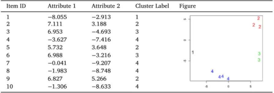
Item ID Attribute 1 Attribute 2 Cluster Label Figure
1 −8.055 −2.913 1 2 7.111 3.188 2 3 6.953 −4.693 3 4 −3.627 −7.416 4 5 5.732 3.648 2 6 6.988 −3.216 3 7 −0.041 −9.207 4 8 −1.983 −8.748 4 9 6.827 5.266 2 10 −1.306 −8.633 4 Table 2
Clustering results of sample dataset.
Case PR (𝜖,MinPts) CD Coef. No. of Clusters
1 0 0 0 0 0 0 0 0 0 0 (9, 7) 0.364 0
2 1 2 3 4 5 6 7 8 9 8 (1, 1) 0.182 9
3 1 2 2 1 2 2 1 1 2 1 (7, 0) 0.667 2
4 0 1 0 2 1 0 2 2 1 2 (6, 3) 0.909 2
Example 1. The three drawbacks of DBSCAN can be illustrated by considering a simple problem of clustering a dataset of 10 items as shown inTable 1. Firstly, to demostrate the parameter setting problem, the two parameters are randomly set for four different cases as shown in Table 2. The clustering result for each case, generated using DBSCAN, is shown inFig. 1. Inspection ofFig. 1indicates that the known clustering shown inTable 1 is not arrived at. The results are also included in Table 2. The second column gives the clustering pattern resultPR, the third column gives the parameter settings, the fourth column gives the obtained Czekanowski Dice (CD) coefficient and the last column the number of clusters. Note that with respect to the CD coefficient, the higher the value the better the clustering result in comparison with the ground truth clustering.
Secondly, to demonstrate the problem of the number of clusters, it can be observed that the numbers of clusters of the four cases are different and not the same as the number of ground truth clusters given inTable 2.
Thirdly, the cluster labels inTable 1cannot be optionally used in the training to perform a classification.
To overcome the first drawback, this paper proposes Particle swarm Optimized Density-based Clustering and Classification (PODCC) to search for the most appropriated parameters for DBSCAN. To overcome the second and third issues, this paper also presents a number fitness functions used in PODCC.
3. Particle swarm Optimized Density-based Clustering and Classification (PODCC)
The proposed Particle swarm Optimized Density-based Clustering and Classification (PODCC) method is based on the ideas of applying PSO [22] and cluster measurement indices to optimize the input param-eter settings for the algorithm. The operation of PODCC is illustrated by the data flow chart given inFig. 2. A parameter value pair is a parti-cle, which means a possible solution. A group of particles are generated in a 2-dimension search space. Given that the positions (X⃖⃖⃗i= (xi1,xi2)) and velocities (V⃖⃖⃗i= (vi1,vi2)) of particles, the previous best particles (P⃖⃖⃗i= (pi1,pi2)) and the local best particle (⃖⃗L= (l1,l2)) are initialized, a loop is executed to find the best particle of the highest fitness value. The loop starts with updatingX⃖⃖⃗iandV⃖⃖⃗i. The updated particles are passed to the DBSCAN function to produce a cluster pattern result (PR). In this paper, a pattern result means either a clustering result or a classifica-tion result. The fitness values ofPRsare computed by chosen fitness functions. Two types of fitness function, unsupervised and supervised, are considered in this paper (the nature of these functions is considered further in Section4). The best particles are updated with respect to the fitness values. To ensure that the process terminates, a maximum iter-ation (T) is specified. The loop will be terminated whenTis reached. FinallyL⃖⃗is returned and used in DBSCAN to produce the Best Pattern Results (BPR).
Algorithm 2 PODCC.
Input: A fitness functionF, dataset, the swarm sizeMand maximum iteration numberT;
Output: Best Pattern ResultBPR;
1. For all particles in the swarm,∀i∈ {1,…,M}
1.1 Initialise particles’ positionsX⃖⃖⃗iand velocitiesV⃖⃖⃗i; 1.2 Initialise personal/previous bestP⃖⃖⃗iand local bestL⃖⃗; 2. For all particles in the swarm,∀i∈ {1,…,M}
2.1 Update particle’s velocity by Eq.(5); 2.2 Update particle’s position by Eq.(9); 2.3 Generate the Pattern Results by
(PR)X⃖⃗ i=DBSCAN(,xi1,xi2); (PR)⃖⃗ Pi=DBSCAN(,pi1,pi2); (PR)⃖⃗ Li=DBSCAN(,l1,l2); 2.4 IfF((PR)X⃖⃗ i)<F((PR)P⃖⃗i), then
Update particle’s best-known position⃖⃖⃗Pi=X⃖⃖⃗i; 2.5 IfF((PR)P⃖⃗
i)<F((PR)⃗L), then
Update the neighbourhood’s best-known positionL⃖⃗=P⃖⃖⃗i; 3. Repeat step 2 until maximum iteration numberTor the other stop condition is met;
4. Generate the best Pattern Result, i.e.BPR= (PR)⃗
L=DBSCAN(,l1,l2).
The pseudo code for PODCC are presented inAlgorithm 2. In this paper the Standard Particle Swarm Optimization algorithm defined in 2011 (SPSO-2011) [22] was used, but clearly alternatives could be sub-stituted. SPSO-2011 was used because the adaptive random topology and rotational invariance featured in SPSO-2011 has been shown to achieve faster convergence to the global optimum than pervious PSO variants.
Returning to Algorithm 2, in Step 1, the particles are initialized using the following equations.
xi,d=U(mind,maxd) (1) vi,d= U(mind,maxd) −x0 i,d 2 (2) pi,d=x0i,d (3) li,d=min(f(p0i,d)) (4)
whereU(mind,maxd)is a random value in[mind,maxd]where the sub-scriptd∈ {1,2}means the dimension of the particle.
In Step 2.1, the velocity is updated using the following function: ⃖⃖⃗
Vi=𝜔⃖⃖⃗Vi+x′−X⃖⃖⃗i (5)
wherex′ is a random point defined in the hypersphere:i(G⃖⃖⃗i,‖G⃖⃖⃗i−
⃖⃖⃗
Xi‖). For theith particle, a centre of gravity (G⃖⃖⃗i) is calculated using three points: the current position (X⃖⃖⃗i), a point slightly beyond the best previous personal position (⃖⃖⃗pi), and a point slightly beyond the best previous position in the neighbourhood (l⃖⃗i), as shown below:
⃖⃖⃗ pi=X⃖⃖⃗i+c1U⃖⃖⃖⃗1⊗(⃖⃖⃗Pi−X⃖⃖⃗i) (6) ⃖⃗ li=X⃖⃖⃗i+c2U⃖⃖⃖⃗2⊗(⃖⃗L−⃖⃖⃗Xi) (7) ⃖⃖⃗ Gi= ⃖⃖⃗ Xi+p⃖⃖⃗i+l⃖⃗i 3 (8)
wherec1andc2are the cognitive and social acceleration coefficients respectively.U⃖⃖⃖⃗1andU⃖⃖⃖⃗2are the predefined independent and uniformly distributed random vectors respectively within the range [0,1]. ⊗
means the element-wise vector multiplication.𝜔is a predefined inertia weight.
In Step 2.2, the position of theith particle are updated according to the equation:
⃖⃖⃗
Xi=X⃖⃖⃗i+V⃖⃖⃗i (9)
In Step 2.3, by using the particlesxi1andxi2as𝜖andMinPts respec-tively, the items in the dataset can be clustered or classified by DBSCAN according toAlgorithm 1given in Section2. In Steps 2.4 and 2.5, the fitness value of the pattern results can be computed by using different fitness functions defined in Section4below. After the stop condition is met, the best pair of parameters,l1andl2, are the output in Step 3. Finally, the optimized pattern results are returned by passing the parameters,l1andl2, as𝜖andMinPtsin DBSCAN.
4. Design of fitness functions for PODCC
A number of fitness functions are designed for either unsupervised or supervised learning using Particle swarm Optimized Density-based Clustering and Classification (PODCC). The fundamental distinction is that if the ground truth target class values of records in the dataset are not used in PODCC we have unsupervised learning (clustering), if they are used we have supervised learning (classification). Both Internal and External Indices are used to measure clustering results. Class labels (ground truth values) are needed for the calculations of external indices, whilst calculations of internal indices do not require ground truth val-ues. The unsupervised fitness function for PODCC,Fusp, is defined as follows:
Fusp=fInt+fNK (10)
wherefIntis an internal clustering index function andfNK(Eq.(15)) is the sum of the function to control the number of clusters (fK) and the noise minimization function (fNoise). Two widely used clustering indices, the Davies-Bouldin (DB) index [32] and Silhouette (SIL) index [33], are used forfIntin this paper. Given a set ofNdata points= (s1,…,sN) assigned toKclustersC= {C1,…,Ci,…,CK}and the centroids of each clustermi,i =1,…,K.Ci= {si
1,…,s
i j,…,s
i
ni}is theith cluster, where ni is the number of data points inCi. The DB index is calculated as follows: fDB=K1 K ∑ i=1 max i′∈{1,…,K},i′≠i{ ei+ei′ ‖mi−m′i‖2 },ei = (1∕ni) ni ∑ j=1 ‖sij−mi‖2 (11)
whereei andei′are the measures of scatter within clustersCi andC′i respectively. The silhouette statistic (SIL) is calculated using:
fSIL= 1 K K ∑ i=1 ( 1 ni ni ∑ j=1 bi j−a i j max(aij,bij) ) ,where (12) aij = 1 ni−1 ni ∑ k=1,k≠j ‖sij−sik‖ (13) bij = min h∈{1,…,K},h≠i { 1 nh nh ∑ k=1 ‖sij−shk‖ } (14) where: (i)aijis the average distance between a data pointsijbelonging to a clusterCiand all other data points inCi, and (ii)bijis the minimum average distance between thejth data point in the clusterCiand all the data points in the other clusters{Ch∶h≠i}. The lower the DB index the better the clustering result, whilst the higher the SIL index the better
Fig. 2.Data flow diagram outlining the operation of PODCC.
the clustering result. By default, PODCC minimizes the fitness value; thereforefIntisfDBor−fSIL.
The functionfIntcannot be solely used as a fitness function since the best internal indices for PODCC do not lead to the best pattern results. As shown inFig. 3, all the data points are clustered in one cluster when eitherfInt = −fSILorfInt =fDBis the only value to be minimized. The details of the two datasets used inFigs. 3–4are given inTable 5 in Section5.
To address this problemfNK is also used, fNK returns the sum of the function for the number of clusters (fK) and the noise minimization function (fNoise).fNKis defined as follows:
fNK =fK+fNoise,where (15) fK = abs(max(PR) −K) K (16) fNoise = card({PRi∈PR∶PRi=0}) N (17)
The variable fK (Eq. (16)) is used to overcome the drawback of DBSCAN, noted in Section2, that the number of clusters cannot be con-trolled by users. In some real cases, theKvalue is a known a priori, but it cannot be used to guide the clustering process in standard DBSCAN. If theKvalue is unknown, the user can assume someKvalues as the input of PODCC. By comparing the optimized clustering results of the
different inputKvalues, the most suitable number of clusters for the dataset can be found. The variablefKis used to calculate the ratio of the absolute difference between the number of clusters as PODCC pro-cedures (i.e. max(PR)) and the number of clusters determined by the user toK. The variablefKcan be minimized to 0 when max(PR) =K. Therefore, the number of clusters in PODCC can be control by the user. The variablefK cannot be solely used as a fitness function since the pattern results shown inFig. 4may be generated by PODCC.
The functionfNoise is used to compute the percentage of noise in pattern results during PODCC, such that it can be used to minimize the amount of noises in the pattern results. The functionfNoise cannot be solely used as a fitness function since all data points are grouped into one cluster (Fig. 3). The functionfNK can be used as a fitness function for unsupervised PODCC (i.e.Fusp =fNK) where no good internal index is suitable for the dataset to be clustered (see more details in Section5). If the ground truth target class values of a dataset are used in PODCC, PODCC can perform⧵classification supervised learning. A supervised fitness function for PODCC,Fspd, is defined as follows:
Fspd=fExt (18)
fExtis the external clustering index function. An external index function measures the similarity between two partitions, Partition 1 and Parti-tion 2. In this case, the set of classes represents the set of clusters in Partition 1 while Partition 2 represents some other pattern results of
Fig. 3.Clustering Pattern Results using PODCC withfIntorfNoiseas the Fitness Function.
Fig. 4.Results Using PODCC withfKas the Fitness Function.
which the quality to be determined. In other words, the similarity of Partition 2 compared to the “ground truth” Partition 1 indicates the accuracy of Partition 2. When considering a pair of points,𝛼and𝛽, in Partitions 1 and 2, there are four possibilities:
•𝛼𝛼: the two points belong to the same cluster in both partitions.
•𝛼𝛽: the two points belong to the same cluster in Partition 1 but not in Partition 2.
•𝛽𝛼: the two points belong to the same cluster in Partition 2 but not in Partition 1.
•𝛽𝛽: the two points do not belong to the same cluster in either parti-tion.
A widely used external index is the Czekanowski-Dice index [34]. This was thus adopted in the supervised fitness function for PODCC. The CD index is defined as follows:
fCD= 2𝛼𝛼
2𝛼𝛼+𝛼𝛽+𝛽𝛼 (19)
The higher the CD index the better the pattern result. Given that PODCC is designed to minimize the fitness value by default,fExt = −fCDwas
used.
A fitness function is chosen on a case-by-case basis. Details con-cerning the process for choosing fitness function is discussed in Section 5. The operation of PODCC with two different fitness functions,fNK andFExt = −fCD, is illustrated inExample 2, using the same dataset in Example 1(given inTable 1).
Example 2. The dataset of 10 data points is presented in Table 1. The swarm size (amount of particles in the swarm) is set to 4 and the maximum iteration is set to 10.Table 3shows the unsupervised PODCC results by using the fitness functionFusp=fNKpresented in Eq.(15). For example, the fitness of the pattern results produced by using the first particle within Loop 1 is computed as follows:
fNK= abs(max(PR) −K) K + card({PRi∈PR∶PRi=0}) N = abs(3−4) 4 + 3 10=0.55 (20)
In this case, convergence is reached in iteration 5 since the best fitness value 0 is reached at the 5th iteration. At the end, 3 particles (Particles 1, 3, 4) reach the best fitness value.
Table 3
Sample results of PODCC applyingfNK.
Iteration Particle ID Pattern Results Parameters Set Fitness
1 1 0 1 2 0 1 2 3 3 0 3 (1.508, 2) 0.55 2 0 0 0 0 0 0 0 0 0 0 (2.054, 7) 2.00 3 0 0 0 0 0 0 0 0 0 0 (2.726, 7) 2.00 4 0 0 0 0 0 0 0 0 0 0 (8.505, 7) 2.00 5 1 1 1 1 1 1 1 1 1 1 1 (8.892, 4) 0.75 2 1 2 3 4 2 3 4 4 2 4 (5.370, 0) 0.00 3 1 2 3 4 2 3 4 4 2 4 (5.389, 0) 0.00 4 1 1 1 1 1 1 1 1 1 1 (9.999, 2) 0.75 10 1 1 2 3 4 2 3 4 4 2 4 (2.767, 0) 0.00 2 1 2 2 1 2 2 1 1 2 1 (7.260, 1) 0.50 3 1 2 3 4 2 3 4 4 2 4 (5.881, 0) 0.00 4 1 2 3 4 2 3 4 4 2 4 (6.293, 1) 0.00 Table 4
Sample results of PODCC applyingfExt = −fCD.
Iteration Particle ID Pattern Results Parameters Set Fitness
1 1 0 1 0 2 1 0 2 2 1 2 (5.034, 3) −0.909 2 0 1 0 2 1 0 2 2 1 2 (4.862, 3) −0.909 3 0 0 0 0 0 0 0 0 0 0 (2.432, 8) −0.364 4 0 0 0 0 0 0 0 0 0 0 (3.058, 6) −0.364 3 1 0 0 0 0 0 0 0 0 0 0 (3.538, 6) −0.364 2 0 0 0 0 0 0 0 0 0 0 (8.170, 6) −0.364 3 1 2 3 4 2 3 4 4 2 4 (4.711, 0) −1.000 4 0 0 0 0 0 0 0 0 0 0 (9.472, 2) −0.364 10 1 1 2 3 4 2 3 4 4 2 4 (4.322, 2) −1.000 2 1 1 1 1 1 1 1 1 1 1 (8.962, 0) −0.364 3 1 2 3 4 2 3 4 4 2 4 (2.733, 1) −1.000 4 0 1 0 2 1 0 2 2 1 2 (3.025, 3) −0.909
Table 4 shows the supervised PODCC results by using the fitness functionFspd = −fCDpresented in Eq. (19). The pairs of the 10 data points are assigned to the four possibilities as below by taking the pat-tern results as Partition 1 and the ground truth partition as Partition 2.
•𝛼𝛼: 10 pairs of points belong to the same cluster in both partitions.
•𝛼𝛽: 0 pair of points belong to the same cluster in Partition 1 but not in Partition 2.
•𝛽𝛼: 2 pairs of points belong to the same cluster in Partition 2 but not in Partition 1.
•𝛽𝛽: 33 pairs of points do not belong to the same cluster in either partition.
The fitness of the pattern results is computed using the above point pair values as follows:
fCD= 2𝛼𝛼 2𝛼𝛼+𝛼𝛽+𝛽𝛼 = 2∗10 2∗10+0+2= 20 22=0.909 (21)
In this case, convergence is reached in iteration 3 since the best fitness value−1 is reached at the 3rd iteration by Particle 3. Half of the parti-cles (Particle 1 and Particle 3) reach the best fitness value and the same pattern result.
5. Experiments
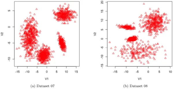
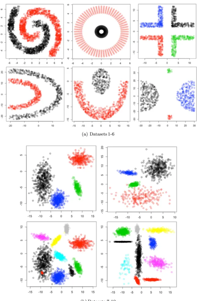
This section presents the results obtained from a sequence of exper-iments used to evaluate the proposed PODCC system. For the experi-ments 10 datasets were used. Comparisons were conducted using com-mon clustering and classification methods. The nature of the datasets used is presented inTable 5. Six of the datasets featured challenging known arbitrary shaped clusters (Datasets 1–6): (i) Two spirals, (ii) Cluster in cluster, (iii) Corners, (iv) Half-kernel, (v) Crescent & Full Moon and (vi) Outlier. The remaining four datasets (Datasets 7–10) were synthetic datasets generated using software provided by Julia
Table 5
Description of 10 datasets.
ID Dataset Name No. of Classes No. of Individuals
1 Two spirals 2 3000
2 Cluster in cluster 2 1024
3 Corners 4 1000
4 Half-kernel 2 1000
5 Crescent & Full Moon 2 1000
6 Outlier 4 600
7 2d-4c-no0 4 1572
8 2d-4c-no2 4 1064
9 2d-10c-no0 10 2972
10 2d-10c-no2 10 3073
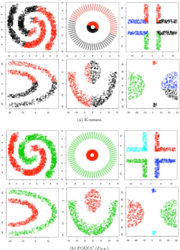
Handl [35]. The “ground truth” partitions of Datasets 1–6 are shown inFig. 5a, and the partitions for Datasets 7–10 are shown inFig. 5b.
Four individual sets of experiments were conducted to evaluate the performance of PODCC. The first three were designed for evaluating PODCC in the context of unsupervised learning, for each experiment, one of the unsupervised fitness functions presented on Section4was used, namely: FNK (Eq. (15)), Fusp with Davies Bouldin Index (Eqs. (10) and (11)) andFuspwith Silhouette Index (Eqs.(10) and (12)). For the evaluation, the performance of PODCC was compared with both DBSCAN and K-means. The fourth set of experiments was designed to evaluate the performance of supervised PODCC using the supervised fitness functionFspd with the Czekanowski-Dice Index (Eqs. (18) and (19)). The performance of supervised PODCC was compared with Sup-port Vector Machine (SVM) classification [36].
For the experiments, the following PODCC settings were used: (i) swarm size of 40, (ii) maximum values of the two particles of 10 and the minimum values of 0, (iii)c1,c2 (the cognitive and social acceleration coefficients) andw(predefined inertia weight) set to 1.193, 1.193 and 0.721 respectively, and (iv) the maximum number of iterations to 50.
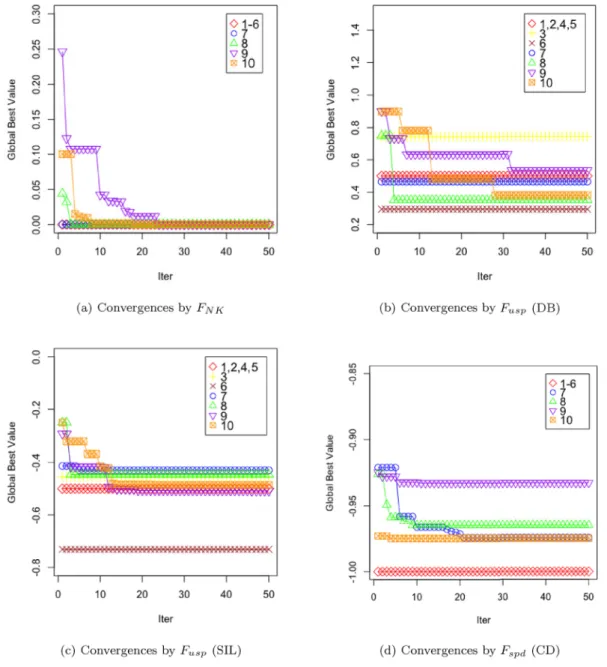
Fig. 6.Convergences of PODCC.
For DBSCAN, the two parameters were set to random values in the range from 0 to 10. For K-means, theKvalue was set according to the given number of clusters for each dataset. For SVM, the default settings using the e1071 package [37] were adopted. For each dataset, the number of times that DBSCAN and K-means were run was set by the product of the swam size times the number of iterations required for PODCC to reach convergence. For example, if the PODCC swarm size was set to 40, and the number of the iterations to reach the convergence point is 24, the number of times DBSCAN and K-means was run should be 40×24=960 times, which is the same as PODCC.
The convergence performance of PODCC in terms of the number of iterations required to reach a stable point is illustrated inFig. 6. From the figure, it can be seen that PODCC converged to a stable state after about 30 iterations. In some cases, PODCC required less than 10 iterations to reach converge. The convergence speed of PODCC should be much faster than in the case of the Genetic Algorithm Density-Based Approach for Clustering (GADAC) [11] which converges at about 100 iterations.
To compare the performance of unsupervised PODCC with DBSCAN and K-means, in terms of accuracy, for each dataset, the average
fit-ness values of the selected fitfit-ness function for all the clustering results (fitavg), the fitness value for the best clustering results (fitbest) and the Czekanowski-Dice indices for the best clustering results (CD) were used. The results are presented inTables 6–8.
Table 6presents the results obtained using PODCC applyingFNKas the fitness function, in comparison to the operation of DBSCAN and K-means. For Dataset 1–6, theCDvalues show that PODCC performs better than DBSCAN and K-means. According to the clustering results shown inFig. A1band the convergence curve shown inFig. 6a, PODCC applyingFNKcan cluster Datasets 1–6 perfectly and in a relatively short time. The fitness values of all the K-means results are 0 usingFNK, asK is known and no noise is contained in the K-means results. Even though the fitness values of the K-means results are minimized, theCDvalues obtained using K-means show that the clustering results are not satis-factory with respect to the ground truth partitions. As the table and Fig. A4bshows, for Datasets 7–10, theCDresults using PODCC apply-ingFNK are not better than K-means, as Datasets 7–10 are obviously centroid-based clustering problems. Although the K-means approach is specifically directed at centroid-based clustering, the operation of k-means is subject to the manner in which the initial cluster centroids are
Table 6
Unsupervised PODCC withFNKversus DBSCAN and K-means.
ID PODCC DBSCAN K-means
fitavg fitbest CD fitavg fitbest CD fitavg fitbest CD
1 0.475 0.000 1.000 1.174 0.000 1.000 0.000 0.000 0.501 2 0.400 0.000 1.000 0.475 0.000 1.000 0.000 0.000 0.645 3 0.716 0.000 1.000 1.045 0.000 1.000 0.000 0.000 0.399 4 1.716 0.000 1.000 0.839 0.000 1.000 0.000 0.000 0.500 5 1.719 0.000 1.000 15.877 0.000 1.000 0.000 0.000 0.567 6 2.019 0.000 1.000 9.392 0.000 1.000 0.000 0.000 0.874 7 4.755 0.000 0.744 0.540 0.000 0.744 0.000 0.000 0.973 8 0.840 0.000 0.715 1.714 0.002 0.836 0.000 0.000 0.929 9 3.441 0.000 0.385 2.340 0.000 0.386 0.000 0.000 0.902 10 1.112 0.000 0.597 1.519 0.002 0.782 0.000 0.000 0.937 Table 7
Unsupervised PODCC with Davies Bouldin index versus DBSCAN and K-means.
ID PODCC DBSCAN K-means
fitavg fitbest CD fitavg fitbest CD fitavg fitbest CD
1 1.632 0.500 0.666 0.834 0.500 0.666 0.931 0.930 0.501 2 4e+15 0.500 0.666 3e+15 0.500 0.666 1.281 1.191 0.645 3 12.794 0.744 1.000 1.226 0.744 1.000 0.750 0.691 1.000 4 16.833 0.500 0.666 2.375 0.500 0.666 0.997 0.997 0.500 5 1.659 0.500 0.769 2.618 0.500 0.769 0.985 0.977 0.567 6 1.112 0.295 0.998 0.659 0.359 1.000 0.652 0.281 0.863 7 1.348 0.465 0.744 5.401 0.714 0.744 0.519 0.310 0.973 8 3.917 0.352 0.715 2.342 0.592 0.836 0.668 0.401 0.929 9 3.312 0.534 0.385 2.046 0.534 0.386 0.512 0.231 0.849 10 1.466 0.382 0.597 1.642 0.482 0.597 0.498 0.258 0.787
generated, and thus the generated cluster results may not be optimal. Examples of the cluster results obtained for Datasets 7–10 are given in Fig. A4a.
The number of clusters (K) cannot be used for DBSCAN. To address this issue, PODCC used withFNKtakesKas input.Figs. A6-A7 demon-strate that different user-definedKvalues for PODCC can lead to differ-ent pattern results. OnceKis smaller than the ground truth number of clusters, 4 in the examples, some small clusters are merged to give big-ger clusters, for example,Figs. A6a, A6b, A7a and A7b. Similarly, when
Kis larger than the ground truth number of clusters, bigger clusters are divided into some smaller clusters, for example,Figs. A6c, A6d, A7c and A7d.
Table 7presents the results of PODCC applying fitness functionFusp with the Davies Bouldin clustering index. From the table, it can be seen that the performance of PODCC is better than DBSCAN for most of datasets considered. The result demonstrates that PODCC can still opti-mize the fitness values with respect to the chosen fitness function; how-ever the presentedCDvalues associated with PODCC are not satisfac-tory for most of the datasets.Figs. A2a and A4cshow the clusters
result-ing from PODCC with Davies Bouldin as the fitness function. Inspection of the figures indicates that the results could be much improved. It can thus be concluded that the DB index is not appropriate in the case of unsupervised PODCC.
Table 8 presents the results of PODCC when a fitness function
Fusp with the Silhouette Index is used. From the table it can be seen that PODCC performs better than DBSCAN for all the datasets consid-ered. For Datasets 1–6, thefitbest values using PODCC are better than those associated with K-means, but theCDvalues are still not satis-factory. For Datasets 7–10, although thefitbest values of K-means are higher than PODCC, theCDvalues of PODCC are better than the cor-responding K-means values for Datasets 9–10. Comparing the results shown inTable 7, using the Silhouette index as the basis for the fitness function achieves the better performance than using Davies Bouldin Index. It can thus be concluded that PODCC can address satisfacto-rily centroid-based clustering problems using a Silhouette based fitness function.
As already noted that supervised PODCC can be used for classifica-tion purposes, to evaluate this, its operaclassifica-tion was compared to SVM in
Table 8
Unsupervised PODCC with silhouette index versus DBSCAN and K-means.
ID PODCC DBSCAN K-means
fitavg fitbest CD fitavg fitbest CD fitavg fitbest CD
1 5.637 −0.500 0.666 −0.453 −0.500 0.666 −0.431 −0.432 0.501 2 −0.435 −0.500 0.666 −0.377 −0.500 0.666 −0.321 −0.376 0.645 3 −0.105 −0.455 1.000 −0.242 −0.455 1.000 −0.419 −0.455 1.000 4 0.724 −0.500 0.666 2.402 −0.500 0.666 −0.413 −0.413 0.500 5 −0.267 −0.500 0.769 0.606 −0.500 0.769 −0.415 −0.420 0.567 6 0.295 −0.731 1.000 0.982 −0.731 1.000 −0.523 −0.594 0.850 7 0.393 −0.430 0.962 1.465 −0.415 0.742 −0.599 −0.686 0.973 8 −0.070 −0.446 0.836 0.542 −0.446 0.836 −0.494 −0.595 0.929 9 0.127 −0.507 0.926 1.125 −0.499 0.909 −0.564 −0.621 0.896 10 0.209 −0.486 0.974 0.367 −0.480 0.971 −0.577 −0.630 0.833
Table 9
Supervised PODCC with Czekanowski-dice index versus SVM.
ID PODCC SVM CDavg BP CDbest CD 1 0.694 (0.576, 5) 1.000 0.980 2 0.733 (1.456, 9) 1.000 1.000 3 0.522 (1.566, 6) 1.000 0.976 4 0.752 (2.180, 4) 1.000 1.000 5 0.846 (3.929, 8) 1.000 1.000 6 0.844 (8.098, 1) 1.000 1.000 7 0.678 (1.189, 10) 0.974 0.922 8 0.659 (1.480, 5) 0.965 0.969 9 0.457 (0.913, 6) 0.933 0.677 10 0.615 (0.628, 4) 0.975 0.542
terms of: (i) the average Czekanowski-Dice Index of all the predicted pattern results (CDavg) in PODCC, (ii) the Best Parameters (BP), (iii) the corresponding CD index values of the best predicted patterns (CDbest) of PODCC, and (iv) the CD index values of the SVM prediction results (CD). The results are presented inTable 9. It can be seen that PODCC performs better than SVM for all datasets except for Dataset 8. How-ever, for Dataset 8 the CD value produced by PODCC is very close to the SVM result. By comparing the pattern results of Dataset 8 given in Figs. A5a and A5b, it can be seen that the boundaries of the classes pro-duced by PODCC are clearer than the SVM results, as PODCC inherits the character of DBCSAN which can find the presence of noises in the datasets. Such character could be either advantage or limitation subject to different situations.
The comparisons between proposed components are presented in Table 10. To summarize, PODCC when using the fitness functionFNK can be applied to datasets featuring arbitrary shaped clusters; whilst classical DBSCAN requires a manual generation and test process to find the appropriate parameters to produce the correct results; K-means cannot find clusters of arbitrary shape at all. PODCC when usingFusp with the Silhouette Index can cluster centroid-based datasets. Accord-ing to the analysis of the experimental results, the combination of PSO, DBSCAN, and fitness function with SIL index leads to the best perfor-mance of the unsupervised PODCC method. Supervised PODCC can deal with all types of labelled datasets. Whilst a suitable fitness function is chosen with respect to dataset, PODCC performs better than DBSCAN and K-means for unsupervised learning and better than SVM for super-vised learning.
6. Simulations
The proposed unsupervised and supervised PODCC methods with different fitness functions have been applied to analyse the open datasets with the classes of overlapped feature values. To compare PODCC with Genetic Algorithm Optimized DBSCAN for Clustering and Classification (GODCC), the SPSO part of PODCC was modified and replaced by a GA using theGA package in R [38,39] to imple-ment GODCC. The performance of unsupervised PODCC was compared with the unsupervised GODCC, standard DBSCAN and K-means, whilst the performance of supervised PODCC was compared with supervised GODCC and SVM.
In this simulation, ten datasets were selected from the open sources. The details of attributes and classes in the ground truth partitions for all the datasets used are summarized inTable 11. Seven datasets were selected from UCI repository [40] (Sonar [41], Zoo [42], Ionosphere [43], Soybean [44], and Sani [45–47]) and R machine learning pack-ages [48] [49], (Hacide [50] and Default [51]).
The other three datasets are the internet traffic datasets of three different sizes which were sampled from several big open datasets regarding TCP packet traces [52], which are the internet traffic clus-tering/classification cases. As the proposed method does not attempt to solve the big data problem, sampling was used. Five features of the datasets were selected to analyse: (1) mean inter-arrival time; (2) mean IP packet size; (3) the total number of packets; (4) the total number of unique bytes sent; and (5) connection duration. The examples were manually classified into different application types, including WWW, mail, p2p, services, interactive, etc.
From the class sizes and distributions shown in Table 11, eight datasets (Zoo, Ionosphere, Sani, Hacide, Default datasets and three traf-fic datasets) can be considered to be imbalanced datasets. Take the dataset Traffic for example; more than 80%of individuals are in one class, and the rest of individuals are in the other nine classes.
For the datasets inTable 11, the PODCC settings were as follows: (i) Swarm size was set to 50; (ii) maximum value of𝜖was the maxi-mum distance among individuals; (iii) maximaxi-mum value ofMinptswas the value of the number of individuals divided by the number of clus-ters; (iv) the minimum values of𝜖andMinptswere 0; (v) c1, c2 (the cognitive and social acceleration coefficients) and w (predefined inertia weight) were set as 1.193, 1.193 and 0.721 respectively; and (vi) the maximum number of iterations was 50. For DBSCAN, the two parame-ters, radius and minpts, were set to random values in the search space
Table 10
The comparisons among k-means, SVM, DBSCAN and different combinations for PODCC.
ID Method Components Clustering Classification Analysis Results
1 K-means K-means Yes Noa It cannot deal with the dataset featuring arbitrary shaped
clusters; The number of clusters can be controlled by the users.
2 DBSCAN DBSCAN Yes Noa It can deal with the dataset featuring arbitrary shaped clusters;
The number of clusters cannot be controlled by the users. 3 Unsupervised PODCC withfNK PSO; DBSCAN;F=fNK Yes Nob It can deal with the dataset consisting of arbitrary shaped
clusters; The number of clusters can be controlled by the users; The accuracy measured by CD Index has been improved comparing to methods 2 and 4.
4 Unsupervised PODCC with DB Index PSO; DBSCAN;F=fDB+ fNK Yes Nob It can deal with the dataset consisting of arbitrary shaped clusters; The number of clusters can be controlled by the users; The accuracy measured by CD Index has been improved comparing to method 2.
5 Unsupervised PODCC with SIL Index PSO; DBSCAN;F=fSIL +fNK Yes Nob It can deal with the dataset consisting of arbitrary shaped clusters; The number of clusters can be controlled by the users; The accuracy measured by CD Index has been improved comparing to methods 1, 2, 3, and 4.
6 SVM SVM No Yes It may not lead to the best result.
7 Supervised PODCC with CD Index PSO; DBSCAN;F=fCD No Yes The accuracy measured by CD Index has been improved comparing to method 6.
a Even the dataset has labelled variable. b The dataset has no labelled variable.
Table 11
Details of the ten evaluation datasets.
Dataset No. of Attributes No. of Individuals No. of Classes Class Sizes Class Distribution Type
Soybean 36 47 4 17/10/10/10 Balanced Sonar 60 208 2 111/97 Balanced Zoo 16 101 7 41/20/13/10/8/5/4 Imbalanced Ionosphere 34 351 2 225/126 Imbalanced Sani 55 303 2 216/87 Imbalanced Hacide 2 1250 2 1225/25 Imbalanced Default 2 10000 2 9667/333 Imbalanced Traffic1K 5 1000 10 831/108/25/11/7/6/5/4/2/1 Imbalanced Traffic2K 5 2000 9 1671/200/56/20/19/14/11/5/4 Imbalanced Traffic5K 5 5000 10 4164/519/138/50/41/39/28/13/5/3 Imbalanced Table 12
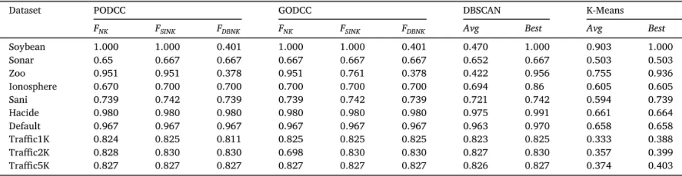
CD index values of clustering results of PODCC, GODCC, DBSCAN, and K-means.
Dataset PODCC GODCC DBSCAN K-Means
FNK FSINK FDBNK FNK FSINK FDBNK Avg Best Avg Best
Soybean 1.000 1.000 0.401 1.000 1.000 0.401 0.470 1.000 0.903 1.000 Sonar 0.65 0.667 0.667 0.667 0.667 0.667 0.652 0.667 0.503 0.503 Zoo 0.951 0.951 0.378 0.951 0.761 0.378 0.422 0.956 0.755 0.936 Ionosphere 0.670 0.700 0.700 0.700 0.700 0.700 0.694 0.86 0.605 0.605 Sani 0.739 0.742 0.739 0.739 0.742 0.739 0.721 0.742 0.594 0.739 Hacide 0.980 0.980 0.980 0.980 0.980 0.980 0.975 0.991 0.661 0.664 Default 0.967 0.967 0.967 0.967 0.967 0.967 0.963 0.970 0.658 0.658 Traffic1K 0.824 0.825 0.811 0.825 0.825 0.825 0.823 0.825 0.333 0.388 Traffic2K 0.828 0.830 0.830 0.698 0.830 0.830 0.827 0.830 0.357 0.399 Traffic5K 0.827 0.827 0.827 0.827 0.827 0.827 0.826 0.827 0.374 0.403
of PODCC. For K-means, the K value was set according to the given number of groups for each dataset. For fair comparisons, DBSCAN and K-means were run for 2500 times. For SVM, the default settings using thee1071 package in R [37] were adopted. For GA, the default settings in theGApackage [38,39] were adopted, but the size of the population and the maximum number of iterations were changed to 50 respectively (same number for PODCC).
Tables 12 and 13present the simulation results of unsupervised and supervised PODCC with the four proposed fitness functions,FNK (Eq (15)),FSINK (Eq.(10)with Eq.(12)),FDBNK (Eq.(10)with Eq. (11)), andFCD(Eq.(18)with Eq.(19)). The accuracy of clustering and clas-sification results was measured by the external CD index with respect to the ground-truth labels.Table 12 presents the results of unsuper-vised PODCC, unsuperunsuper-vised GODCC, DBSCAN andK-means for the ten datasets. By comparing the CD index values of the clustering results, it can be found that the accuracy of unsupervised PODCC applyingFNKor FSINKis better than or equal to the average accuracy of DBSCAN, and the best accuracy ofK-means.
In Table 12, whilst the unsupervised PODCC achieves the simi-lar accuracy as the GODCC for most cases, the accuracy of PODCC withFSINK for the dataset Zoo and PODCC with FNK for the dataset
Traffic2K is significantly higher than the GODCC results. The major reason that PODCC performs better than GODCC is that PODCC adopted SPSO 2011, which performs better than GA for optimizing continuous functions [14] and more efficiently than GA [15]. Regard-ing continuous optimal solution, Fig. 7a demonstrates that PODCC searches the better optimal value than GODCC. Regarding computa-tional efficiency,Fig. 7b demonstrates that PODCC converges faster than GODCC.
Table 13presents the results of supervised PODCC withFCD, super-vised GODCC withFCD, and SVM for the ten datasets. Both Full Train Full Prediction (FTFP) test and 90% training set and 10%prediction set (9T1P) test were conducted for each algorithm. FTFP means that all data are used for training and prediction, and 9T1P means that 90%of data was used to build a training model and the remaining 10%data was used for prediction.
Supervised PODCC and GODCC withFCDachieved almost the same results for all the datasets due to sufficient searching iteration for the best results. For the datasets, Sonar, Zoo, Ionosphere, Hacide, and Default, the accuracy of SVM prediction results is higher than both PODCC and GODCC, but both Supervised PODCC and GODCC perform better than SVM for the three internet traffic datasets, whilst all of the
Table 13
CD index values of classification results of PODCC, GODCC and SVM.
Dataset PODCC GODCC SVM
FTFP 9T1P FTFP 9T1P FTFP 9T1P Soybean 1.000 1.000 1.000 1.000 1.000 1.000 Sonar 0.667 0.667 0.667 0.667 0.917 0.802 Zoo 0.955 0.956 0.955 0.956 1.000 0.944 Ionosphere 0.861 0.853 0.861 0.853 0.984 0.974 Sani 0.742 0.742 0.742 0.742 0.742 0.742 Hacide 0.991 0.991 0.991 0.991 0.993 0.992 Default 0.971 0.970 0.971 0.970 0.972 0.972 Traffic1K 0.825 0.825 0.825 0.825 0.809 0.662 Traffic2K 0.830 0.831 0.830 0.831 0.825 0.727 Traffic5K 0.827 0.827 0.827 0.827 0.827 0.811
Fig. 7.Convergences of PODCC and GODCC for two cases.
methods achieve the same prediction results for the datasets, Soybean and Sani. Although not all the supervised PODCC outperformed the SVM, a notable superiority of PODCC can be found as below. PODCC achieved better prediction results in the 9T1P test than in the FTFP. For SVM, the accuracy of FTFP results is higher or equal to the 9T1P results; the 9T1P results for datasets Sonar, Traffic1K, and Traffic2K are significantly worse than the FTFP results. For PODCC, the accu-racies of FTFP and 9T1P results are similar. For datasets Traffic2K and Zoo, the 9T1P results of PODCC are slightly higher than its FTFP results.
By comparing the results of different datasets in the two tables, it can be found that both PODCC and GODCC can achieve better pattern results for the eight imbalanced datasets than the others. The accuracy of unsupervised PODCC results for the imbalanced datasets is signifi-cantly higher than theK-means results; and the supervised PODCC for three internet traffic dataset significantly outperforms SVM when 9T1P is applied. In PODCC, the data points in the big size class can be grouped into one class if they are in the close hyper-spheres determined by the appropriate parameters for DBSCAN, whilst the big size class can be forced to be divided into several small classes regardless of the density of data points inK-means.
Overall, the analysis comes to three conclusions.
•Unsupervised PODCC with FNK andFSINK can find better cluster-ing results than K-means. In the experiments, the PSO applied in DBSCAN clustering method performs better than GA in some cases (Zoo and Traffic2K).
•For the selected cases in this paper, the 9T1P setting for the super-vised PODCC is likely to have better prediction results than the FTFP setting, whilst 9T1P is more frequently used and practical than FTFP.
•PODCC is recommended for the imbalanced clustering and classifi-cation problems. For the simulation of some imbalanced datasets, the PODCC has better performance in clustering and classification thanK-means and SVM respectively.
7. Conclusions
This paper proposes a novel method, Particle Swarm Optimized Density-Based Clustering and Classification (PODCC) to overcome the three drawbacks of classical Density-Based Spatial Clustering of Appli-cations with Noise (DBSCAN). Firstly the two critical parameters for DBSCAN are difficult to set; secondly when using DBSCAN the
num-ber of desired clusters cannot be pre-specified by the user; and thirdly DBSCAN cannot be used in a supervised learning context where labelled training data can be used to drive the clustering. To address the first drawback, a Particle Swarm Optimization (PSO) based approach is pro-posed to search the entire parameter space for DBSCAN. The second drawback is addressed by using proposed fitness functions that take the number of desired clusters into account. The third drawback is addressed by another proposed fitness function, one that operates with labelled training data, so that PODCC can also perform in a supervised learning context.
The proposed PODCC system was evaluated using 10 datasets; com-parisons were undertaken so as to analyse the operation of the proposed fitness functions, and to analyse the operation of PODCC in comparisons to DBSCAN, K-means and SVM. The experiment results show that the unsupervised PODCC performs better than DBSCAN and K-means, and that supervised PODCC can perform better than SVM when a suitable fitness function is chosen.
Ten open datasets with the classes of overlapped feature values were used to evaluated PODCC. To compare with PODCC, Genetic Algo-rithm Optimized DBSCAN for Clustering and Classification (GODCC) was proposed. The SPSO part of PODCC was modified and replaced by a GA to implement GODCC. The performance of unsupervised PODCC was compared with the unsupervised GODCC, standard DBSCAN and K-means, whilst the performance of supervised PODCC was compared with supervised GODCC and SVM. The results obtained indicated that unsupervised PODCC can find better clustering results thanK-means and GODCC, when a suitable fitness function is chosen. Both unsuper-vised and superunsuper-vised PODCC methods are found to be appropriate for both imbalanced clustering and classification problems.
For future work, the idea is to extend PODCC as a framework for ESA optimized DBSCAN clustering and classification. More comprehensive comparisons between different ESAs in optimizing the parameters of DBSCAN will be conducted. Since the advantage of DBSCAN is that it finds the arbitrary shaped clusters, the application of ESA optimized DBSCAN methods will be explored in the area of image processing, such as face recognition and medical image segmentation.
Acknowledgement
The research work reported in this paper is partially supported by Research Grants from the National Natural Science Foundation of China (Project Number 61503306) and the Natural Science Foundation of Jiangsu Province (Project Number BK20150377), China.
Appendix
Fig. A7PODCC Results of Dataset 8 with Different Numbers of Clusters Defined by the User.
References
[1] J. Han, J. Pei, M. Kamber, Data Mining: Concepts and Techniques, Elsevier, 2011. [2] F. Lotte, M. Congedo, A. Lecuyer, F. Lamarche, B. Arnaldi, A review of́
classification algorithms for eeg-based brain–computer interfaces, J. Neural. Eng. 4 (2) (2007) R1.
[3] M. Ester, H.-P. Kriegel, J. Sander, X. Xu, et al., A density-based algorithm for discovering clusters in large spatial databases with noise, in: Kdd, vol. 96, 1996, pp. 226–231. no. 34.
[4] D.B. Fogel, Evolutionary Computation: toward a New Philosophy of Machine Intelligence, vol. 1, John Wiley & Sons, 2006.
[5] J. Kennedy, Particle swarm optimization, in: Encyclopedia of Machine Learning, Springer, 2011, pp. 760–766.
[6] D. Karaboga, An Idea Based on Honey Bee Swarm for Numerical Optimization, Technical report-tr06, Erciyes university, engineering faculty, computer engineering department, Tech. Rep., 2005.
[7] M. Dorigo, V. Maniezzo, A. Colorni, Ant system: optimization by a colony of cooperating agents, IEEE Trans. Syst., Man, Cybern., Part B (Cybernetics) 26 (1) (1996) 29–41.
[8] D.E. Golberg, Genetic Algorithms in Search, Optimization, and Machine Learning, vol. 1989, Addion wesley, 1989, p. 102.
[9] R. Storn, K. Price, Differential evolution–a simple and efficient heuristic for global optimization over continuous spaces, J. Global Optim. 11 (4) (1997) 341–359. [10]H. Jiang, J. Li, S. Yi, X. Wang, X. Hu, A new hybrid method based on
partitioning-based dbscan and ant clustering, Expert Syst. Appl. 38 (8) (2011) 9373–9381.
[11]C.-Y. Lin, C.-C. Chang, C.-C. Lin, A new density-based scheme for clustering based on genetic algorithm, Fundam. Inf. 68 (4) (2005) 315–331.
[12] A. Karami, R. Johansson, Choosing dbscan parameters automatically using differential evolution, Int. J. Comput. Appl. 91 (7) (2014) 1–11.
[13] S. Bandyopadhyay, U. Maulik, Nonparametric genetic clustering: comparison of validity indices, IEEE Trans. Syst. Man Cybern. C Appl. Rev. 31 (1) (2001) 120–125.
[14] H. Zhou, M. Song, W. Pedrycz, A comparative study of improved ga and pso in solving multiple traveling salesmen problem, Appl. Soft Comput. 64 (2018) 564–580.
[15] AIAA, A comparison of particle swarm optimization and the genetic algorithm, in: Aiaa/asme/asce/ahs/asc Structures, Structural Dynamics & Material Conference, 2005, pp. 833–843.
[16] D. Van der Merwe, A.P. Engelbrecht, “Data clustering using particle swarm optimization, in: Evolutionary Computation, 2003. CEC’03. The 2003 Congress on, vol. 1, IEEE, 2003, pp. 215–220.
[17] C.-Y. Chen, F. Ye, Particle swarm optimization algorithm and its application to clustering analysis, in: Networking, Sensing and Control, 2004 IEEE International Conference on, vol. 2, IEEE, 2004, pp. 789–794.
[18] X. Cui, T.E. Potok, P. Palathingal, Document clustering using particle swarm optimization, in: Proceedings 2005 IEEE Swarm Intelligence Symposium, 2005. SIS 2005, IEEE, 2005, pp. 185–191.
[19] T. Niknam, B. Amiri, An efficient hybrid approach based on pso, aco and k-means for cluster analysis, Appl. Soft Comput. 10 (1) (2010) 183–197.
[20] R. Xu, J. Xu, D.C. Wunsch, A comparison study of validity indices on swarm-intelligence-based clustering, IEEE Trans. Syst., Man, Cybern., Part B (Cybernetics) 42 (4) (2012) 1243–1256.
[21] R. Xu, J. Xu, D.C. Wunsch, Clustering with differential evolution particle swarm optimization, in: IEEE Congress on Evolutionary Computation, IEEE, 2010, pp. 1–8.
[22]M. Zambrano-Bigiarini, M. Clerc, R. Rojas, Standard particle swarm optimisation 2011 at cec-2013: a baseline for future pso improvements, in: 2013 IEEE Congress on Evolutionary Computation, IEEE, 2013, pp. 2337–2344.
[23]P. Viswanath, R. Pinkesh, l-dbscan: a fast hybrid density based clustering method, in: 18th International Conference on Pattern Recognition (ICPR’06), vol. 1, IEEE, 2006, pp. 912–915.
[24]D. Birant, A. Kut, St-dbscan: an algorithm for clustering spatial–temporal data, Data Knowl. Eng. 60 (1) (2007) 208–221.
[25]P. Viswanath, V.S. Babu, Rough-dbscan: a fast hybrid density based clustering method for large data sets, Pattern Recogn. Lett. 30 (16) (2009) 1477–1488. [26]S. Kisilevich, F. Mansmann, D. Keim, P-dbscan: a density based clustering
algorithm for exploration and analysis of attractive areas using collections of geo-tagged photos, in: Proceedings of the 1st International Conference and Exhibition on Computing for Geospatial Research & Application, ACM, 2010, p. 38.
[27]Y. He, H. Tan, W. Luo, H. Mao, D. Ma, S. Feng, J. Fan, Mr-dbscan: an efficient parallel density-based clustering algorithm using mapreduce, in: Parallel and Distributed Systems (ICPADS), 2011 IEEE 17th International Conference on, IEEE, 2011, pp. 473–480.
[28]M.M.A. Patwary, D. Palsetia, A. Agrawal, W.-k. Liao, F. Manne, A. Choudhary, A new scalable parallel dbscan algorithm using the disjoint-set data structure, in: High Performance Computing, Networking, Storage and Analysis (SC), 2012 International Conference for, IEEE, 2012, pp. 1–11.
[29]T.N. Tran, K. Drab, M. Daszykowski, Revised dbscan algorithm to cluster data with dense adjacent clusters, Chemometr. Intell. Lab. Syst. 120 (2013) 92–96. [30]G. Andrade, G. Ramos, D. Madeira, R. Sachetto, R. Ferreira, L. Rocha, G-dbscan: a
gpu accelerated algorithm for density-based clustering, Procedia Comput. Sci. 18 (2013) 369–378.
[31]A. Lulli, M. Dell’Amico, P. Michiardi, L. Ricci, Ng-dbscan: scalable density-based clustering for arbitrary data, Proceedings of the VLDB Endowment, vol. 10, 2016, pp. 157–168. no. 3.
[32]D.L. Davies, D.W. Bouldin, A cluster separation measure, IEEE Trans. Pattern Anal. Mach. Intell. (2) (1979) 224–227.
[33]P.J. Rousseeuw, Silhouettes: a graphical aid to the interpretation and validation of cluster analysis, J. Comput. Appl. Math. 20 (1987) 53–65.
[34]J. Czekanowski, Zur differentialdiagnose der Neandertalgruppe. Friedr, Vieweg & Sohn, 1909.
[35]J. Handl, J. Knowles, Improvements to the scalability of multiobjective clustering, in: 2005 IEEE Congress on Evolutionary Computation, vol. 3, IEEE, 2005, pp. 2372–2379.
[36]C. Cortes, V. Vapnik, Support-vector networks, Mach. Learn. 20 (3) (1995) 273–297.
[37] D. Meyer, E. Dimitriadou, K. Hornik, A. Weingessel, F. Leisch, e1071: Misc functions of the department of statistics (e1071), tu wien. r package version 1.6-3, Retrieved from, 2014.
[38] L. Scrucca, Ga: a package for genetic algorithms in r, J. Stat. Software 53 (4) (2013) 1–37.
[39] L. Scrucca, On some extensions to ga package: hybrid optimisation, parallelisation and islands evolution, R J. 9 (1) (2017) 187–206.
[40] D. Dheeru, E. Karra Taniskidou, UCI Machine Learning Repository, 2017. [Online]. Available:http://archive.ics.uci.edu/ml.
[41] R.P. Gorman, T.J. Sejnowski, Analysis of hidden units in a layered network trained to classify sonar targets, Neural Network. 1 (1) (1988) 75–89.
[42] C.B.D. Newman, C. Merz, UCI Repository of Machine Learning Databases, 1998. [Online]. Available:http://www.ics.uci.edu/_mlearn/MLRepository.html. [43] V.G. Sigillito, S.P. Wing, L.V. Hutton, K.B. Baker, Classification of Radar Returns
from the Ionosphere Using Neural Networks, vol. 10, 1989.
[44] R.S. MICHALSKI, Learning by being told and learning from examples: an experimental comparison of the two methods of knowledge acquisition in the context of development an expert system for soybean disease diagnosis, Int. J. Pol. Anal. Inf. Syst. 4 (1) (1980) 515–528.
[45] R. Alizadehsani, J. Habibi, M.J. Hosseini, H. Mashayekhi, R. Boghrati, A. Ghandeharioun, B. Bahadorian, Z.A. Sani, A data mining approach for diagnosis of coronary artery disease, Comput. Methods Progr. Biomed. 111 (1) (2013) 52–61. [46] R. Alizadehsani, M.H. Zangooei, M.J. Hosseini, J. Habibi, A. Khosravi, M.
Roshanzamir, F. Khozeimeh, N. Sarrafzadegan, S. Nahavandi, Coronary artery disease detection using computational intelligence methods, Knowl. Base Syst. 109 (C) (2016) 187–197.
[47] Z. Arabasadi, R. Alizadehsani, M. Roshanzamir, H. Moosaei, A.A. Yarifard, Computer aided decision making for heart disease detection using hybrid neural network-genetic algorithm, Comput. Methods Progr. Biomed. 141 (C) (2017) 19–26.
[48] G. James, D. Witten, T. Hastie, R. Tibshirani, ISLR: Data for an Introduction to Statistical Learning with Applications in R, 2013. r package version 1.0. [Online]. Available:https://CRAN.R-project.org/package=ISLR.
[49] N. Lunardon, G. Menardi, N. Torelli, ROSE: a package for binary imbalanced learning, R J. 6 (1) (2014) 82–92.
[50] G. Menardi, N. Torelli, Training and assessing classification rules with imbalanced data, Data Min. Knowl. Discov. 28 (1) (2014) 92–122.
[51] J.Z. Huang, An Introduction to Statistical Learning: with Applications in R by Gareth James, Trevor Hastie, Robert Tibshirani, Daniela Witten, vol. 19, 2014, pp. 556–557.
[52] C. Yang, F. Wang, B. Huang, Internet traffic classification using dbscan, in: 2009 Wase International Conference on Information Engineering, 2009, pp. 163–166.