Using rule extraction to improve the comprehensibility of
predictive models
Johan Huysmans, Bart Baesens and Jan Vanthienen
DEPARTMENT OF DECISION SCIENCES AND INFORMATION MANAGEMENT (KBI)
Faculty of Economics and Applied Economics
Using Rule Extraction to Improve the
Comprehensibility of Predictive Models
Johan Huysmans, Bart Baesens and Jan Vanthienen
Katholieke Universiteit Leuven
Department of Decision Sciences and Information Management
Naamsestraat 69, 3000 Leuven, Belgium
Abstract
Whereas newer machine learning techniques, like artificial neural net-works and support vector machines, have shown superior performance in various benchmarking studies, the application of these techniques remains largely restricted to research environments. A more widespread adoption of these techniques is foiled by their lack of explanation capability which is required in some application areas, like medical diagnosis or credit scor-ing. To overcome this restriction, various algorithms have been proposed to extract a meaningful description of the underlying ‘black box’ models. These algorithms’ dual goal is to mimic the behavior of the black box as closely as possible while at the same time they have to ensure that the extracted description is maximally comprehensible.
In this research report, we fist develop a formal definition of ‘rule extraction’ and comment on the inherent trade-off between accuracy and comprehensibility. Afterwards, we develop a taxonomy by which rule extraction algorithms can be classified and discuss some criteria by which these algorithms can be evaluated. Finally, an in-depth review of the most important algorithms is given. This report is concluded by pointing out some general shortcomings of existing techniques and opportunities for future research.
1
Introduction
1.1
Definition
Whereas there already exist various definitions of ‘rule extraction’, we believe that most of these are too restrictive. For example, Craven [13] defines rule extraction as:
“Given a trained neural network and the data on which it was trained, pro-duce a description of the network’s hypothesis that is comprehensible yet closely
approximates the network’s prediction behaviour.”
which is reformulated in [10] as:
“In the scenario of high dimensional feature spaces, given a trained SVM and the data on which it was trained, produce a description of the SVM’s hypothesis that is understandable yet closely approximates the SVM’s prediction behavior”
Both definitions view the process of rule extraction from their specific field of interest, respectively neural networks and SVMs. However, the above defini-tions of rule extraction can be formulated more generally as:
“Given an opaque predictive model and the data on which it was trained, produce a description of the predictive model’s hypothe-sis that is understandable yet closely approximates the predictive model’s behavior”
PSfrag replacements
X Y
(a) Better Comprehensibility
PSfrag replacements
X Y
(b) Better Accuracy
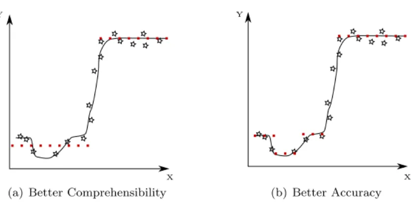
Figure 1: Trade-off between Accuracy and Comprehensibility (full line=original model, dotted line=extracted rules)
A first issue to notice from this definition is that although the process is coined ‘rule extraction’, it is not required that the returned description con-sists of rules. We consider any method that delivers a human-comprehensible description of the underlying model as a rule extraction technique. Although most algorithms will indeed provide a description consisting of rules, there exist techniques that provide descriptions in different formats such as decision trees, finite state machines or graphical models. The term ‘white box extraction’ might therefore be more appropriate than the widespread term ‘rule extraction’.
From the above definitions, one can also observe the inherent duality between comprehensibility and accuracy1. The extracted description should be
compre-hensible but at the same time approximate the underlying model as closely as
1
possible. Which of both goals is favored usually depends on the specific require-ments of the application. For example, in Figure 1, a regression model (full line) is built from the available sample observations. In the left figure, a simple model (dotted line) of the following form is extracted:
if X is smaller than threshold then Y is Value1
else Y is Value2
While this rule set provides a relatively good approximation of the underlying model, there are some minor deviations between the original model and the extracted rules. Figure 1(b) shows a rule set that better approximates the underlying model.
if X is smaller than threshold1 then Y is Value1
if X∈[threshold1,threshold2] then Y is Value2
if X∈[threshold2,threshold3] then Y is Value3
else Y is Value4
This rule set is however more elaborate and contains twice the amount of rules as the first rule set. Which of both rule sets is preferred, usually depends on the specific requirements of the application at-hand.
During our review of rule extraction algorithms, this trade-off between accu-racy and comprehensibility will be encountered several times. Most algorithms deal with the duality by allowing users to set some parameters to specify a desired level of accuracy or a maximum level of complexity.
1.2
Motivation
At this point, one might start wondering why rule extraction is important. If it is of major concern to have a good understanding of the predictive model, it seems logical to avoid the intermediate step of creating an opaque model and to start directly with a ‘white box’ model.
The main motivation is that a well trained intermediate model can often better represent the data than the data itself by filtering out the noise that is present in the samples. Additionally, the use of the intermediate ‘black box’ model allows the creation of ‘artificial’ data examples for those regions of the input space that are covered by only a small number of sample points. Finally, several benchmarking studies [5, 54, 57] have shown that in many application areas opaque models achieve better performance than ‘white box’ models. In situations where performance is a crucial issue, the opaque models are there-fore the preferred choice for implementation in the decision process but rule extraction can be adopted to verify the knowledge encoded in these models.
This knowledge verification is crucial in many application areas and some-times even legally required. For example, the Equal Credit Opportunity Act [1] is a US federal law which prohibits creditors from certain forms of discrim-ination. Under this law, financial institutions are required to provide specific
reasons in case an application is rejected: indefinite and vague reasons for de-nial are illegal [33]. An unacceptable motivation is for example: “You didn’t receive enough points on our credit scoring system”, which is pretty much the only possible explanation that can be provided by a ‘black box’ scoring system when no rule extraction is performed.
Similar requirements can also be found in the medical domain, where users are reluctant to use ‘black box’ computer-aided diagnosis (CAD) systems that can influence patient treatment [21]. The ability to generate even limited ex-planations is essential for user acceptance of such systems.
Apart from the explanation capability, several other reasons that underline the importance of rule extraction are mentioned in [3]. Automatic knowledge acquisition is one of them. Constructing and debugging a knowledge base for a decision support system is a difficult and time-consuming task. Automatic rule-extraction can considerably facilitate the burden of maintaining such knowledge base. Other possible motivations for rule extraction are the induction of scien-tific theories or the study of the generalization behavior of the underlying model.
1.3
Rule Types
As discussed above, most of the extraction algorithms generate rules to describe the underlying model’s hypothesis. Many different types of rules exist. In this section, we provide an overview of several frequently used rule types.
The most widespread rules are without any doubt propositional if-then rules. The condition part of a propositional rule is a boolean combination of conditions on the input variables. Whereas the condition part can contain conjunctions, disjunctions and negations, most algorithms will return rules that only contain conjunctions. An example of such a rule is: ‘if X=a and Y=b then Class=1’, with X,Y input variables and a,b possible values of these variables. For continuous input variables, the conditions are usually specified as restrictions on the allowed values, e.g ‘X∈[c1, c2]’ or ‘X> c3’ withc1,c2,c3 ∈R.
Most algorithms will ensure that the condition parts of each rule demarcate separate areas in the input space: i.e. the rules are mutually exclusive. There-fore, only one rule can be satisfied when a new observation is presented and the rule that has fired will be the only one used for making the classification (or regression) decision. However, some algorithms will allow multiple rules to fire for the same instance. This requires an additional mechanism to combine the individual predictions. For example, [10] associates a confidence factor with each rule and rules that fire with a large confidence factor have a greater impact on the final decision. Sorting the rules and allowing only the first firing rule to decide is another mechanism, applied in [51].
M-of-N rules are closely related to propositional rules. They are ex-pressions of the form ‘if {at least/exactly/at most} M of the N conditions
{C1, C2, . . . , CN} are satisfied then Class=1’. It is usually straightforward to convert M-of-N rules into propositional rules. For example, the M-of-N rule ‘if exactly 2-of-{X=a,Y=b,Z=c}then Class=1’ is logically equivalent to ‘if ((X=a and Y=b) or (X=a and Z=c) or (Y=b and Z=c)) then Class=1’. Observe that
for M=1, the rules can be written as a number of disjunctions while for M=N the rules can be expressed as a conjunction of the conditions. The use of M-of-N rules was first proposed in [56]. Other algorithms that provide M-of-N rules as result of their extraction process are the popular TREPAN [15] and FERNN [44].
A third type of rules, which can not be transformed straightforwardly into propositional rules, areoblique rules. Oblique rules represent piecewise dis-criminant functions and are usually represented as follows: ‘if (c1X+c2Y> c3)
and (c4X+c5Z> c6) and . . .then Class=1’ withc1, . . . , c6∈R. In comparison
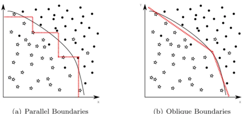
with propositional rules, oblique rules are usually more difficult to understand. However, oblique rules have the advantage that they can create decision bound-aries that are non-parallel with the axes of the original input space. In [48], it is argued that oblique rules may therefore require fewer conditions than propo-sitional rules. An example is shown in Figure 2.
X Y
(a) Parallel Boundaries
X Y
(b) Oblique Boundaries
Figure 2: Parallel versus Oblique Boundaries
In the left part of this figure, the decision boundary is approximated with three propositional rules (or as one rule with three disjunctions in the condition part). The right part shows the approximation of the decision boundary by an oblique rule. We can observe that the same level of accuracy would require a large number of propositional rules.
However, when categorical attributes are present in the data oblique rules become even less interpretable. In [43], this problem is alleviated by the ex-traction of a hierarchical rule set that combines opaque and propositional rule characteristics. Only rules that are low in the hierarchy have conditions that involve linear combinations of continuous attributes while the conditions of all the other rules contain solely discrete attributes. It is argued that such rule conditions greatly increase the comprehensibility of the rules.
Very similar to oblique rules, but slightly more complex, areequation rules. This type of rules was proposed in [36], and contain a polynomial equation in the condition part. An example is : ‘ifc1X2+c2Y2+c3XY +c4X+c5Y < c6
that particular study. It is difficult to understand them and they therefore contribute little to the interpretation of the underlying model.
A fifth type of rules are fuzzy rules. An example of a fuzzy classification rule is: ‘if X is low and Y is medium then Class=1’, whereby low and medium are fuzzy sets with corresponding membership functions. Fuzzy rules are believed to be both comprehensible and user-friendly because the rules are expressed in terms of linguistic concepts, which are easy to interpret for the human expert.
A final category are rules expressed in First Order Logic, i.e. rules that can contain quantifiers and variables. At this moment, we are however not aware of any algorithms that can extract such rules directly and we will therefore not cover this category in more detail.
2
Taxonomy of Rule Extraction Algorithms
In this section, we develop a taxonomy that can be used for discussion and evaluation of rule extraction algorithms. Although there already exists a widely used taxonomy, the ADT -Taxonomy2 proposed in [3], we believe that a new
classification schema may be required to cover the algorithms that extract rules from black box models other than neural networks. The ADT-Taxonomy in-cludes several elements, e.g. translucency and portability, that are specifically defined for neural networks. This makes it less suitable for classifying extraction algorithms that assume other models, such as SVMs (e.g. [36]).
The taxonomy that we propose, contains three main criteria for evaluation of algorithms: the scope of use, the type of dependency on the black-boxand theformat of the extracted description. The latter two of these criteria are also present in the ADT-taxonomy, but as explained below with a different interpretation.
The first dimension concerns the scope of use of an algorithm: either regres-sion or classification. While there are a few algorithms that are applicable for both types of problems, e.g. G-REX [25] and ITER [23], the majority is specifically designed for either one of those. This dimension was included in the taxonomy because it gives an immediate indication about the appropriateness of an algorithm for a specific application. The inclusion of this criterion in the ADT-Taxonomy was also proposed in [4].
The second dimension focuses on the dependency of the extraction algorithm on the underlying black box: independent versus dependentalgorithms. We define a rule extraction algorithm asindependentif it is totally independent of the underlying black box model. It is therefore possible to use the same al-gorithm in combination with different types of opaque models, such as neural networks, support vector machines or an ensemble learner. The only require-ment is that the underlying model can be queried. It acts as an oracle that provides predictions for the observations that it receives. The basic idea is to use the ‘black box’ model as an example-generator from which the algorithm can learn. This added layer of complexity -first training a model on the data and
2
then extracting rules from the model- has often proven advantageous in com-parison with direct rule extraction from the data points. The motivation is that a well trained model can often better represent the data than the original data set [33]. Additionally, the use of the ‘black box’ model allows the creation of ‘artificial’ data examples for those regions of the input space where not enough original data points are available.
Algorithms that use information about the inner-workings of the underlying model aredependent. A dependent algorithm can only be applied if the un-derlying model is of a certain form. Knowledge about the inner-workings of the underlying model can then be used for creation of rules. For example, in [45] the behavior of a regression neural network is converted into regression rules by approximating the activation function of the hidden neurons by a combination of linear functions. For support vector machines, dependent techniques usually rely on the support vectors for the extraction of their rules (e.g., [36]). The main disadvantage of these dependent algorithms is that these techniques pose strict restrictions on the underlying models: they assume that certain activa-tion funcactiva-tions are used or that the architecture of the neural network follows a certain specification.
Readers familiar with the literature on rule extraction, will probably see the similarity of the above distinction with the translucency dimension in the ADT-Taxonomy [3]. The translucency dimension is used to describe the relationship between the extraction algorithm and the internal architecture of the underlying neural network. It makes a distinction betweendecompositional and peda-gogical techniques3. A decompositional technique focuses on the individual units (neurons) within the network and aggregates the rules extracted at the individual levels into a composite rule set. Pedagogical techniques are different because they do not extract rules for the individual neurons but create rules that map the inputs directly into outputs. During our evaluation of the differ-ent rule extraction algorithms, we will observe that there is a large overlapping between dependent and decompositional algorithms and also between indepen-dent and pedagogical algorithms. The overlapping is however not complete. For example, the VIA-algorithm [52] is an example of a pedagogical algorithm. It creates rules by propagating intervals through the network. Because it uses in-formation about the weights of the neural network during the propagation step, VIA can not be applied to other models than neural networks. VIA is therefore a dependent technique.
In the rest of this report, we will use all of the above terms to refer to the translucency of the algorithms. If we state that an algorithm is decompositional then it automatically implies that the algorithm is dependent. Unless explicitly stated otherwise, we will also assume that the term ‘pedagogical’ implies the ‘independence’ of the extraction technique.
While the above distinction between dependent and independent algorithms is useful for the classification of rule extraction techniques, a third criterion that focuses more on the obtained rules might be worthwhile: predictive versus
de-3
scriptive algorithms. We call a rule extraction algorithmpredictive when the extracted rules allow the analyst to make a prediction for each possible obser-vation from the input space. More specifically, every possible input obserobser-vation should be covered by exactly one rule, which means that the extracted rules should be both exclusive and exhaustive. By having both exclusive and exhaus-tive rules, the order in which the rules are processed is of no importance. For classification problems, exhaustivity is often realized by creating only rules for the minority class and adding an additional rule that specifies a default class when the input observation was not covered by any of the other rules. While this imposes a partial ordering on the rules, we consider these rule sets as pre-dictive because it is relatively straightforward to convert them into prepre-dictive rules. Algorithms that extract decision trees are also examples of predictive techniques.
If the rule sets created by a rule extraction algorithm are not predictive, then we call it a descriptive algorithm. The resulting rules are either not-exhaustive or not-exclusive. Non-exhaustivity might provide problems as there will be input observations for which none of the rules fires and no forecast can be delivered. Non-exclusivity might also provide problems because observations can be covered by multiple rules when non-exclusive rules are present. This requires an additional mechanism to combine the individual predictions. For example, [10] associates a confidence factor with each rule and rules that fire with a large confidence factor have a greater impact on the final decision. Sorting the rules and allowing only the first firing rule to decide is another mechanism, applied in [51]. To avoid these problems, users will often prefer the use of predictive algorithms over descriptive algorithms.
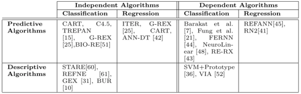
An overview of this taxonomy together with the categorization of several algorithms is shown in Table 1.
Independent Algorithms Dependent Algorithms
Classification Regression Classification Regression Predictive Algorithms CART, C4.5, TREPAN [15], G-REX [25],BIO-RE[51] ITER, G-REX [25], CART, ANN-DT [42] Barakat et al. [7], Fung et al. [21], FERNN [44], NeuroLin-ear [48], RE-RX [43] REFANN[45], RN2[41] Descriptive Algorithms STARE[60], REFNE [61], GEX [31], BUR [10] SVM+Prototype [36], VIA [52]
3
Overview of rule Extraction Algorithms
3.1
Evaluation Criteria
In existing surveys [3, 16, 35], rule extraction algorithms are evaluated by a number of criteria. Besides the characteristics used during creation of the tax-onomy, such as the expressive power of the extracted rules and applicability of the algorithm, several other criteria appear in almost all of these surveys:
• Quality of the extracted rules
• Scalability of the algorithm
• Consistency of the algorithm
We will discuss each of these criteria in greater detail below.
3.1.1 Quality of the Extracted Rules
Quality of the extracted rules is considered to be the most important evaluation criterion for rule extraction algorithms [35]. Many different aspects contribute to the aspect of rule quality: accuracy, fidelity, comprehensibility,...
The concept of accuracy describes whether the extracted rules can make correct predictions for previously unseen test examples. Fidelity is closely related to accuracy, and measures the ability of the extracted rules to mimic the behavior of the model from which they were extracted.
Let {xi, yi}Ni=1 represent observations with their corresponding label and
yBB
i andyW Bi the predictions made by respectively the underlying (Black Box) model and the extracted rules (White Box).
For classification problems, accuracy is usually measured as the percentage of correctly classified observations. More formally, the percentage of observations for whichyiandyiW Bare the same. Fidelity is then expressed as the percentage of observations for whichyBB
i andyW Bi are the same.
accuracyW B=P rob(yi=yW Bi |xi ∈X) (1)
f idelityW B=P rob(yiBB=yW Bi |xi∈X) (2) For regression problems, accuracy is usually measured by the mean-absolute or mean-squared error. These can also be adopted to measure the fidelity be-tween the underlying model and the rules extracted from it. More formally, using the definition of mean-absolute error (MAE):
accuracyW B = 1 N N X i=1 |yi−yiW B| (3) f idelityW B = 1 N N X i=1 |yBB i −yW Bi | (4)
In [59], it is argued that in certain situations it might be impossible to extract rules that have both high accuracy and high fidelity: a situation that is called the fidelity-accuracy dilemma. Consequently, authors must make a choice for either fidelity or accuracy. We are convinced that this dilemma is mainly caused by a badly trained black box model. When extracting rules from a largely overfitted model one might indeed face this problem, but if the underlying model correctly identifies the decision boundaries we see no reason for this dilemma to arise.
A third factor that is of major importance in determining the quality of the extracted rules is theircomprehensibility. Although the main motivation of rule extraction is to obtain a comprehensible description of the underlying model’s hypothesis, this aspect of rule quality is often overlooked. We believe that this is mainly due to the subjective nature of comprehensibility, which can not be measured independently of the person using the system [35]. Prior experience and domain knowledge of this person play an important role in com-prehensibility. This contrasts with accuracy or fidelity that can be considered as properties of the rules and which can be evaluated independently of the users.
In most studies, model complexity is used as a proxy for model comprehen-sibility. The number of rules, the average number of antecedents, the number of leaf nodes of the decision tree, etc. are hereby used as indicators for the model comprehensibility.
3.1.2 Scalability of the algorithm
One desirable characteristic of a rule extraction algorithm is that it can be put in practice on a wide range of applications. This means that an algorithm should not only be able to deal with toy problems, but that it should also remain appli-cable to large-scale problems, i.e. when faced with a large number of examples or input features. Based on [16], scalability in the context of rule extraction can be defined as:
Scalability refers to how the running time of a rule-extraction algorithm and the comprehensibility of its extracted models vary as a function of such factors as the underlying model, the size of the training set and the number of input features
Besides including the traditional notion of scalability, i.e. running time or
algorithmic complexity, the above definition also places emphasis on the as-pect of comprehensibility. The extracted model should remain comprehensible, even if there are many input features and/or training examples. Let us denote this aspect of scalability as non-algorithmic or comprehensibility com-plexity. During the in-depth review of several prominent algorithms, we will observe that many of these algorithms were not developed with non-algorithmic complexity in mind. For example, most neural network decompositional al-gorithms construct rules based on the weights within the neural network and the size of the extracted rule set is usually proportional to the total number of weights [16]. Feature selection and severe pruning of weights and hidden
neu-rons is therefore crucial to obtain a comprehensible description. Pruning is also necessary to reduce the running time of these algorithms as most of them show worst-case exponential behavior [2].
3.1.3 Consistency of the algorithm
A final issue in the evaluation process is the consistency of the algorithm. There are however multiple definitions of this concept. In [3, 56], an algorithm is deemed consistent if under different training sessions, rule sets are generated that produce the same classification of unseen examples. Slightly different is the definition in [35] which labels consistency as the ability of an algorithm to extract rules with the same degree of accuracy under different training sessions. Whereas an algorithm that is consistent according to the first definition is au-tomatically also consistent according to the second definition, the opposite is not necessarily true: rule sets with similar accuracy face the same number of misclassifications but the actual misclassifications can be different. Both defi-nitions are similar in the fact that they only focus on the predictions from the extracted rules and ignore the rules themselves. According to the definition of consistency by Johansson et al. [27], similarity of the extracted rules is however the key aspect:
An algorithm is consistent if it extracts similar rules every time it is applied to the same data set.
However, the author immediately points to the difficulty associated with this definition: there is no straightforward definition of similarity that is applicable for the wide range of representations used in rule extraction. In the discussion below we present a method that we believe is general enough to measure the similarity between two rule sets (or other representation forms) for a given number of observations.
We believe that it is desirable for a measure of similarityσbetween two rule sets to have the following properties:
• similarity between A and B should be equal to similarity between B and A (symmetric)
σ(A, B) =σ(B, A)
• If the two rule sets are exactly the same then the similarity should be maximal.
σ(A, A) = 1
• If the two rule sets provide different classifications for each input observa-tion then the similarity should be minimal
σ(A,¬A) = 0
We propose the following algorithm to calculate the similarity σ between two rule sets A and B, given N input observations.
1. Assign a unique identifier to each rule of A and B
2. For each observation: find the prediction made by set A and B and the identifiers of the rules of A and B that were used to make this prediction 3. For each rule r in A and B. Find the observations for which the classifica-tion decision was based on r. Denote this number of observaclassifica-tions withNr. For each rule in the other rule set that predicts the same class as r, find the identifier of the rule s that fired most frequently for these observations. Denote the number of times that rule s fired asNopposite
r 4. Use as similarity measure the sum of all theNopposite
r divided by the sum of allNr. σ(A, B) = P r∈A,BNropposite P r∈A,BNr = 1 2N X r∈A,B Nopposite r (5)
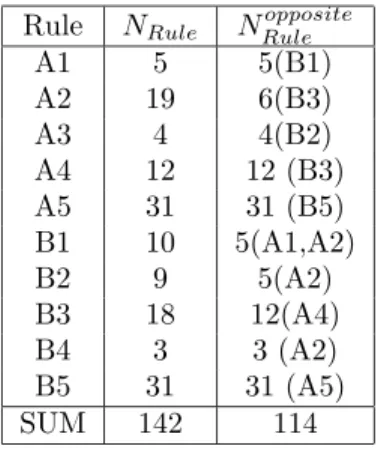
We will clarify the above algorithm with the example shown in Figure 3. An algorithm has provided two rule sets to divide the BLACK from the WHITE observations. We first assign each rule a unique identifier: A1,. . . ,A5 and B1,. . . ,B5. For this example, we will assume that all rules, except A5 and B5, predict the class to be BLACK. We can observe from the figure that A and B create the same decision boundary between the two classes and they will therefore make exactly the same predictions for all observations. This means that they are completely consistent according to the first two definitions. We will show how the rule sets are only partially consistent when applying the third definition and the algorithm described above.
X Y PSfrag replacements A1 A2 A3 A4 A5:default=white B1 B2 B3 B4 B5:default=white α β γ ψ ω (a) Rule Set A
X Y PSfrag replacements A1 A2 A3 A4 A5:default=white B1 B2 B3 B4 B5:default=white α β γ ψ ω (b) Rule Set B Figure 3: Consistency
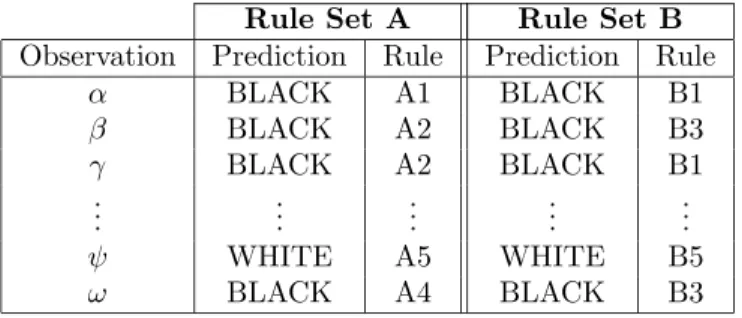
In the second step of the algorithm Table 2 is constructed. For each obser-vation, this table contains the predictions made by each rule set and the rule identifier of the rule that fired for the observation.
This table is used during the third step of the algorithm. For each rule, we first query the table to find out how many times the rule fired, e.g. NA1 = 5
andNB1 = 10. Afterwards, the algorithm looks for the rule in the other rule
set that provides the same classification for most of these observations. In this example, all observations are classified the same by both rule sets, thus we only have to find the rule in the other rule set that fires the most. Because all 5 examples classified by rule A1 are classified by rule B1,NAopposite1 = 5. For the 10 observations classified by rule B1, we can observe that half are classified by A1 and the other half by A2: NBopposite1 =5. The same calculation is repeated for all the rules and the results of this step are shown in Table 3. The division of the totals in this table gives us a similarity estimate of 80%. It is not easy to give an intuitive meaning to this number, but the above procedure can be considered more or less as assigning to each rule a corresponding rule of the other rule set and the similarity measure is then the proportion of examples that were classified by corresponding rules.
Rule Set A Rule Set B
Observation Prediction Rule Prediction Rule
α BLACK A1 BLACK B1 β BLACK A2 BLACK B3 γ BLACK A2 BLACK B1 .. . ... ... ... ... ψ WHITE A5 WHITE B5 ω BLACK A4 BLACK B3
Table 2: Consistency: step 2
It is straightforward to alter the above algorithm to make it applicable to other representation forms, such as decision trees or decision tables. The only required change is in the first step of the algorithm. Instead of the assignment of an identifier to each rule, we will assign identifiers to each leaf-node for decision trees or to each column if the representation format is a decision table. The only assumption for the remainder of the algorithm is that each classification decision is based on exactly one identifier, i.e. the rules must be mutually ex-clusive (non-overlapping). This requirement is automatically fulfilled by various representation formats, such as decision trees and decision tables.
The proposed consistency measure is also not limited to classification prob-lems only. With minor changes, the above algorithm can also be applied to mea-sure consistency on regression problems. However, this requires an additional parameter s to indicate the desired level of sensitivity. Instead of requiring the corresponding rules to predict the same class, the sensitivity measure is used with regression problems to decide whether the predictions of corresponding
Rule NRule NRuleopposite A1 5 5(B1) A2 19 6(B3) A3 4 4(B2) A4 12 12 (B3) A5 31 31 (B5) B1 10 5(A1,A2) B2 9 5(A2) B3 18 12(A4) B4 3 3 (A2) B5 31 31 (A5) SUM 142 114
Table 3: Consistency: step 3
rules are similar enough. Therefore, in the third step we would replace “For each rule in the other rule set that predicts the same class as r” by “For each rule in the other rule set that provides the same forecast within s-difference as r”.
In most application areas, accuracy is probably much more important than consistency: the individual rules are unimportant as long as the rule set provides the correct classification. One might even argue that algorithms with low con-sistency are preferred as they might provide different views on the same data. In other domains the opposite situation may be encountered: consistency plays a pivotal role when explicatory power is the main requirement. Johansson [27] formulates this as follows: “it is very hard to give any significance to a specific rule set if the extracted rules vary significantly between runs.”
3.2
Independent Algorithms
The main advantage of this category of algorithms is their independence of the underlying black box model. Although most algorithms in this category were originally conceived to extract rules from neural networks they remain applicable when the underlying model changes to a support vector machine or any other black box technique.
3.2.1 Rule Learners: CN2
Many algorithms are capable of learning rules directly from a set of training examples, e.g. CN2 [11], AQ [34], RIPPER [12]. Because of their ability to learn rules directly from data, these algorithms are not considered to be rule extraction techniques in the strict sense of the word. However, these algorithms can also be used to extract a human-comprehensible description from opaque models. When used for this purpose, the original target values of the training
SEQUENTIAL-COVERING(Class, Attributes, Examples, Threshold) 1 RuleSet= ∅
2 Rule =LEARN-ONE-RULE(Class, Attributes, Examples) 3 While (Performance(Rule)>Threshold)
4 RuleSet=RuleSet∪Rule
5 Examples = Examples -{examples correctly classified by Rule} 6 Rule= LEARN-ONE-RULE(Class, Attributes, Examples) 7 End While
8 Sort RuleSet according to performance of the rules 9 Return RuleSet
Figure 4: Sequential Covering
examples are modified by the predictions made by the black box model and the algorithm is then applied on this modified data set.
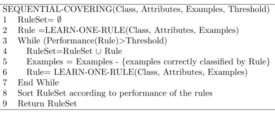
In this section, we discuss a general class of rule learners: sequential covering algorithms. This series of algorithms extracts a rule set by learning one rule, removing the data points covered by that rule and reiterating the algorithm on the remainder of the data. The general outline of sequential covering algorithms is given in Figure 4.
Starting from an empty rule set, the sequential covering algorithm first looks for a rule that is highly accurate for predicting a certain class. If the accuracy of this rule is above a user-specified threshold, then the rule is added to the set of already found rules and the algorithm is repeated over the rest of the examples that were not classified correctly by this rule. If the accuracy of the rule is below this threshold the algorithm will terminate. Because the rules in the rule set can be overlapping, the rules are first sorted according to their accuracy on the training examples before they are returned to the user. New examples are classified by the prediction of the first rule that was triggered.
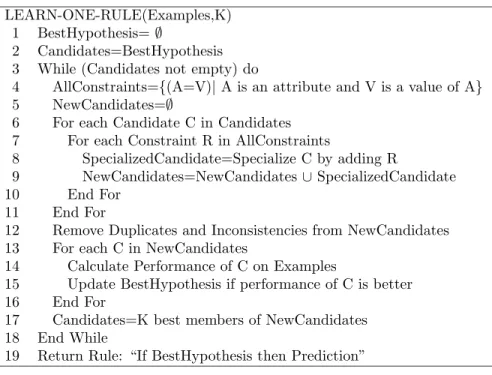
It is clear that in the above algorithm, the subroutine LEARN-ONE-RULE is of crucial importance. The rules returned by the routine must have a good accuracy but do not necessarily have to cover a large part of the input space. The exact implementation of LEARN-ONE-RULE will be different for each algorithm but usually follows either a bottom-up or top-down search process. If the bottom-up approach is followed, the routine will start from a very specific rule and drops in each iteration the attribute that least influences the accuracy of the rule on the set of examples. Because each dropped condition makes the rule more general, the search process is also called specific-to-general search. The opposite approach is the top-down or general-to-specific search: the search starts from the most general hypothesis and adds in each iteration the attribute that most improves accuracy of the rule on the set of examples. This approach was followed in the CN2 algorithm [11] which is shown in Figure 5.
This LEARN-ONE-RULE implementation starts from the most general hy-pothesis and performs a beam search with a beam width of K. At each iteration
LEARN-ONE-RULE(Examples,K) 1 BestHypothesis=∅
2 Candidates=BestHypothesis 3 While (Candidates not empty) do
4 AllConstraints={(A=V)|A is an attribute and V is a value of A} 5 NewCandidates=∅
6 For each Candidate C in Candidates 7 For each Constraint R in AllConstraints
8 SpecializedCandidate=Specialize C by adding R
9 NewCandidates=NewCandidates∪SpecializedCandidate
10 End For
11 End For
12 Remove Duplicates and Inconsistencies from NewCandidates 13 For each C in NewCandidates
14 Calculate Performance of C on Examples
15 Update BestHypothesis if performance of C is better
16 End For
17 Candidates=K best members of NewCandidates 18 End While
19 Return Rule: “If BestHypothesis then Prediction” Figure 5: Learn-One-Rule: CN2 implementation
the best K hypotheses are remembered and used as starting point for special-ization during the next iteration. When the algorithm terminates, it will return the best hypothesis it has found together with the class label that corresponds to the majority class of the examples covered by this hypothesis.
As can be observed from line 4, the algorithm assumes that the attributes are categorical and creates tests of the form: Atribute=value. Consequently, for continuous attributes a discretization is required. Often this discretization will be performed once to the entire data set before the sequential covering algorithm is executed (global discretization). The same intervals will therefore appear in multiple rules which might be beneficial for the interpretability of the rule set. A second option is the application of local discretization. Local discretization is performed during the subroutine LEARN-ONE-RULE and is based on the examples that were provided as input to this routine. The same variable will therefore be discretized several times during execution of the algorithm and different interval conditions will appear in the rule set.
3.2.2 Decision Trees: C4.5 and CART
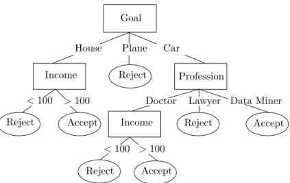
Decision trees [9, 37, 29] are widely used in predictive modeling. A decision tree is a recursive structure that contains a combination of internal and leaf nodes. Each internal node specifies a test to be carried out on a single variable and its branches indicate the possible outcomes of the test. An observation can
PSfrag replacements
Income Income
House Plane Car
>100 >100 Accept Accept Accept Reject Reject Reject Reject Goal <100 <100 Profession Lawyer
Doctor Data Miner
Figure 6: An Example Decision Tree
be classified by following the path from the root towards a leaf node. At each internal node, the corresponding test is performed and the outcome indicates the branch to follow. With each leaf node, a value or class label is associated. An example decision tree is shown in Figure 6. This fictious tree can be used by financial institutions to decide whether or not to accept loan applications.
Just like the rule learners discussed in the previous section, decision trees are usually constructed directly from the available training observations and are therefore not considered to be rule extraction techniques in the strict sense of the word. However, it is also possible to apply these techniques for pedagogical rule extraction by replacing the original targets with the target values provided by the trained black box model. The tree can then be trained on these new data points. If trees are used as an extraction technique, the observations that were wrongly predicted by the underlying model are usually not used during training. Additionally, random instances can be created and added to the training set. For example, in [6] a support vector machine is built from the original training data. A second data set is randomly generated with class labels for each instance provided by the support vector machine. Both data sets are then combinedly used to train a C5 decision tree4.
In the rest of this section, we discuss briefly the two most widespread algo-rithms for decision tree induction: C4.5 for classification problems and CART for regression problems.
C4.5 [37] is one of the most popular algorithms for the construction of decision trees. It uses a divide-and-conquer approach to construct a suitable
4
tree from a set of training examples. LetS be the set of training examples that reach a node t. The approach will then recursively apply the following steps:
• IfS contains only examples from the class C, then t is a leaf-node and it is assigned the class C.
• If S contains no examples, then t is a leaf node. Some heuristic must be used to provide a class label to t. C4.5 will assign this leaf the most frequent class at the parent of this node.
• S contains examples that belong to a mixture of classes. In that case, the algorithm must select a test, based on a single attribute, to split the setS into smaller subsetsS1,. . . ,SN. Each of these subsets will contain all the examples ofS that have the same outcome for this test. The algorithm is then recursively applied to each of the new sets.
One important step is not yet clarified: the selection of the test in case
S contains observations from a mixture of classes. Ideally, we would like the algorithm to find the optimal test, i.e. the test that provides us with the smallest possible tree. Unfortunately, finding the optimal tree is NP-complete and in most cases computationally infeasible. A greedy-heuristic is used to overcome this problem. At each step, we select that attribute and test that produces the ‘purest’ subsets. An often used measure for the impurity of a node is the entropy. Entropy for the setS containing observations from C different classes is defined as: Entropy(S) =− C X i=1 pilog2(pi) (6)
with pi the proportion of examples of class i in the node. We can observe that the entropy serves well as an impurity measure: it is minimal when all observations in S belong to the same class and maximal when all classes are equally likely. From all possible tests T that divide the set S into subsets
S1,. . . ,SN, the algorithm will select the testT∗ that maximizes:
Gain(S,T) =Entropy(S)− N X i=1 |Si| |S|Entropy(Si) (7)
with|S| representing the number of observations in S. The testT∗ is thus
selected such that the weighted entropy in the subsets is minimal. Maximal-ization of the Information Gain has however one serious deficiency: it favors tests with many outcomes. The Gain Ratio criteria adjusts the bias by using a normalization term Inf o(S,T) =− N X i=1 |Si| |S|log2 |Si| |S| (8)
and maximizing the following Gain Ratio
GainRatio(S,T) = Gain(S,T)
Inf o(S,T) (9)
In principle, the recursive splitting can be continued until each leaf node contains only one observation. This strategy would however lead to an overly complex tree with many internal and leaf nodes that overfits the training data. A more parsimonious tree can often be found that provides better generaliza-tion performance. Earlier work tried to obtain such a parsimonious tree by not dividing a node if the improvement achieved by the best test was smaller than some predefined threshold [22, 37]. This approach suffers however from the fact that the greedy approach looks only one step ahead. It is possible that the improvement at this step is only small, while the step after it could lead to a substantial improvement. Early stopping is therefore no longer used by most induction algorithms, but replaced by a separate pruning phase. After construction of the largest possible tree, the pruning phase recursively merges leaf nodes until the best possible tree is obtained. C4.5 uses a heuristic based on the binomial distribution to decide whether pruning will improve generalization behavior of the tree or not.
A second very popular tree induction algorithm isCART, short for Classifi-cation and Regression Trees [9]. We will only discuss the version of CART used for induction of regression trees. The variant for classification trees is largely similar to C4.5, but with a different splitting criterion (Gini Index) and pruning procedure.
A CART regression tree [9] is a binary tree with conditions specified next to each non-leaf node. Classifying a new observation is done by following the path from the root towards a leaf node, choosing the left node when the condition is satisfied and the right node otherwise, and assigning to the observation the value below the leaf node. This value below the leaf nodes equals the average y-value of training observations falling into this leaf node. Variants [28] of CART allow the predictions of the leaf nodes to be linear functions of the input variables.
Similarly to a classification tree, the regression tree is constructed by iter-atively splitting nodes, starting from only the root node, so as to minimize an impurity measure. Often, the impurity measure for regression problems of a node t is calculated as:
R(t) = 1
N
X
xn∈t
(yn−y(t))2 (10)
with (xn, yn) the training observations and y(t) the average y-value for ob-servations falling into node t. The best split for a leaf-node of the tree is chosen such that it minimizes the impurity of the newly created nodes. Mathematically, the best split s* of a node t is that split s which maximizes:
with tL and tR the newly created nodes andpL and pR the proportion of examples sent to respectively tL and tR. Pruning of the nodes is performed afterwards to improve generalization behavior of the constructed tree. Pruning in CART is performed by a procedure called ‘minimal cost complexity pruning’ which assumes that there is a cost associated with each leaf-node. We will briefly explain the basics behind this pruning mechanism, more details can be found in [9, 29]. By assigning a cost αto each leaf node, we can consider the total cost of a tree to consist of two terms: the error rate of the tree on the training data and the cost associated with the leaf nodes.
Cost(Tree)= Error(Tree) +αNumberLeafNodes(Tree) (12) For different values of α, the algorithm first looks for the tree that has a minimal total cost. For each of these trees, the algorithm estimates the error on a separate data set that was not used for training and remembers the value of
αthat resulted in the tree with minimal error. A new tree is then constructed from all available data and subsequently pruned based on this optimal value of
α. In case there is only limited data available, a slightly more complex cross-validation approach is followed, for which the details are provided in [9].
3.2.3 TREPAN
TREPAN [13, 15] is a popular pedagogical rule extraction algorithm. While it is limited to classification problems, it is able to deal with both continu-ous and nominal input variables. TREPAN shows many similarities with the more conventional decision-tree algorithms that learn directly from the training observations, but differs in a number of respects.
First, when constructing conventional decision trees, a decreasing number of training observations is available to expand nodes deeper down the tree. TREPAN overcomes this limitation by generating additional instances. More specifically, TREPAN ensures that at least a certain minimum number of obser-vations are considered before assigning a class label or selecting the best split. If fewer instances are available at a particular node, additional instances will be generated until this user-specified threshold is met. The artificial instances must satisfy the constraints associated with each node and are generated by taking into account each feature’s marginal distribution. So, instead of taking uniform samples from (part of) the input space, TREPAN first models the marginal dis-tributions and subsequently creates instances according to these disdis-tributions while at the same time ensuring that the constraints to reach the node are sat-isfied. For discrete attributes, the marginal distributions can easily be obtained from the empirical frequency distributions. For continuous attributes, TREPAN uses a kernel density based estimation method [50] that calculates the marginal distribution for attribute x as:
f(x) = 1 m m X i=1 1 √ 2πσe −(x−2σµi)2 (13)
with m the number of training examples,µi the value for this attribute for example i and σ the width of the gaussian kernel. TREPAN sets the value for σ to 1/√m. One shortcoming of using the marginal distributions is that dependencies between variables are not taken into account. TREPAN tries to overcome this limitation by estimating new models for each node and using only the training examples that reach that particular node. These locally estimated models are able to capture some of the conditional dependencies between the different features. The disadvantage of using local models is that they are based on less data, and might therefore become less reliable. TREPAN handles this trade-off by performing a statistical test to decide whether or not a local model is used for a node. If the locally estimated distribution and the estimated distribution at the parent are significantly different, then TREPAN uses the local distributions, otherwise it uses the distributions of the parent.
Second, most decision tree algorithms, e.g. CART [9] and C4.5 [37], use the internal (non-leaf) nodes to partition the input space based on one simple feature. Trepan on the other hand, uses M-of-N expressions in its splits that allow multiple features to appear in one split. Remember from Section 1.3 that an M-of-N split is is satisfied when M of the N conditions are satisfied.
2-of-{a,¬b,c} is therefore logically equivalent to (a ∧ ¬b) ∨(a ∧ c) ∨(¬b ∧c). To avoid to test all of the possible large number of M-of-N combinations, TREPAN uses a heuristic beam search with a beam width of 2 to select its splits. The search process is initialized by first selecting the best binary split at a given node based on the information gain criteria([13] (or gain ratio according to [15]). This split and its complement are then used as basis for the beam search procedure that is halted when the beam remains unchanged during an iteration. During each iteration, the following two operators are applied to the current splits:
• m-of-n+1: the threshold remains the same but a new literal is added to the current set. For example, 2-of-{a,b}is converted into 2-of-{a,b,c} • m+1-of-n+1: the threshold is incremented by one and a new literal is
added to the current set. For example, 2-of-{a,b} is converted into
3-of-{a,b,c}
Thirdly, while most algorithms grow decision trees in a depth-first manner, TREPAN employs the best-first principle. Expansion of a node occurs first for those nodes that have the greatest potential to increase the fidelity of the tree to the network.
A final difference between TREPAN and more conventional decision tree algorithms concerns the stopping criteria used by TREPAN to decide when to stop growing the tree. Conventional algorithms will first construct a complete tree and prune this tree afterwards. TREPAN on the other hand uses both local and global criteria to decide on the optimal tree. Local criteria only take the current node into account, such as the number of training instances or their class distribution, to decide whether or not to expand the current node. The local criterion uses by TREPAN is based on the purity of the tree. A node will become a leaf if, with a high probability, it only covers examples from a single
class. TREPAN will create a confidence interval and calculate the number of instances necessary to be able to decide whetherP(propc<1−²)< αwith α a significance level and²an indication of how tight the interval must be.
Besides such a local criterion TREPAN also employs global criteria. Unlike local criteria, global criteria take the entire tree into account and not only the node currently considered for expansion. TREPAN allows the user to specify a complexity parameter, a maximum number of internal nodes, as global criterion to limit the size of the tree returned by TREPAN. Additionally, a validation data set can be provided. TREPAN uses this set to measure the fidelity of each tree created and returns the tree with the highest fidelity.
3.2.4 ANN-DT and DecText
TheANN-DT(Artificial Neural Network Decision Tree) algorithm is described by its authors as ‘an algorithm that extracts binary decision trees from a trained neural network’ [42]. Although the name of the algorithm suggests a close inter-twining of the extraction algorithm with the underlying neural network, ANN-DT does not place any restrictions on the structure of this underlying model and is therefore also applicable with other types of black box classifiers. Addi-tionally, ANN-DT can be applied to data sets where both inputs and outputs can be discrete or continuous. In the rest of this section, we discuss the variant of the algorithm developed for regression problems [42].
ANN-DT shares the idea of TREPAN to sample the input space to create additional training instances. The sampling method used is however different from TREPAN’s that was based on the features’ marginal distributions. ANN-DT randomly generates instances but only keeps those instances for which the distance towards the nearest original training observation is smaller than some predefined critical value. This ensures that only data points are created that resemble the original training data. The critical distance is determined by select-ing a large enough sample of the trainselect-ing data and takselect-ing the average distance between these points and their 10 nearest neighbors. The new instances are then presented to the ‘black box’, from which a predicted output is obtained.
Afterwards, a binary decision tree is constructed from these artificial in-stances by recursively splitting the input space based on one of the input at-tributes. Two different variants of ANN-DT exist that differ in the selection method of the best attribute to split on and an appropriate threshold. The first variant, ANN-DT(e), makes these choices such that the weighted variance in the newly created branches is minimized. This is the same criterion as used in CART’s regression trees. The second variant, ANN-DT(s), is computationally more expensive and selects as splitting attribute the feature that has most sig-nificance on the behavior of the underlying model. The mathematical details can be found in [42], but the idea behind this type of feature selection is to find the attribute a that has the largest significanceσ(f)afor the black box function f(x) at the current branch. For significant attributes, changes in the attribute’s value will be related to variation in the function.
divides the current input space in two subspaces. Growing of the tree is termi-nated when the variance in a node becomes zero or when one of the stopping criteria is satisfied. A first (local) stopping criteria is to expand a node only when the mean outputs of the instances in each of the two children are signif-icantly different from each other. This is tested with an F-test for all nodes below a user-specified minimum depth in the tree. Similarly to TREPAN, users can also specify a global complexity parameter: the maximum depth of the tree. Nodes at this level will not be further expanded.
Empirical studies conclude that ANN-DT had similar or better performance than those obtained from CART. The ANN-DTT(s) variant with significance analysis to select the splitting attribute, was found to provide more accurate rules.
DecText[8], short for Decision Tree Extractor, is very similar to TREPAN and ANN-DT. It was designed specifically for the extraction of a classification decision tree from a neural network and to obtain this goal several different splitting criteria were proposed. We will briefly discuss one of these criteria, SetZero, and the pruning mechanism.
The SetZero splitting method tries to find the attribute that has most effect on the outputs of the underlying model. This is similar to the idea behind ANN-DT(s) but differs in how the split is actually calculated. First, for all of the observations that fall in a specific node, the underlying model is queried to find the corresponding outputs. Then, the algorithm places the value of the first attribute to zero in all the observations and queries the network again to find its predictions for these mutated inputs. This process is repeated for each of the possible attributes and the absolute difference between the original outputs and the mutated outputs indicates how much the outcome is affected by the attribute. The algorithm will select the attribute with the largest influence. One can observe that the SetZero splitting mechanism can only be applied if there is an underlying model that can provide predictions for the mutated observations. It can therefore not be applied directly on training data.
Besides the special splitting criterion, DecText also uses a special pruning mechanism, called Fidelity Pruning. First, a number of random observations is created and the corresponding output is obtained from the black box. Pruning of leaf nodes is then performed as long as it improves the fidelity on this random data set.
3.2.5 GEX and G-REX
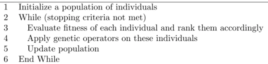
Various approaches based on the ubiquitous genetic algorithms have been pro-posed to tackle the problem of rule extraction. In this section, we will discuss GEX [31] and G-REX [25], (both abbreviations for ‘Genetic Rule EXtraction’) as examples of this approach. In Figure 7, the basic idea behind genetic algo-rithms is explained.
First, a random population of individuals is created. Each individual rep-resents a possible solution to the proposed problem. For rule extraction, an
1 Initialize a population of individuals 2 While (stopping criteria not met)
3 Evaluate fitness of each individual and rank them accordingly 4 Apply genetic operators on these individuals
5 Update population 6 End While
Figure 7: The Basic Genetic Algorithm
individual will therefore correspond with a rule or a rule set. Afterwards, the algorithm will calculate a level of fitness for each individual. This problem-specific fitness function is used to measure how well an individual is able to solve the corresponding problem. For rule extraction, the fitness measure will incorporate elements such as accuracy and comprehensibility of the rule (set). Consequently, two individuals will be selected to create offspring whereby in-dividuals that are fitter than others will have a greater probability of being selected. Their children will inherit elements from both parents and form a new and updated population. Some of the parents will also be added directly to this updated population: either unchanged or with slight mutations. The general idea is Darwin’s survival of the fittest: small mutations and inheritance will give increasingly better solutions to solve the original problem. The algorithm will stop when a maximum number of iterations is reached or when an individual is found that is sufficiently fit.
GEX[31] follows the general approach of a genetic algorithm, but differs on several aspects. The first difference is that GEX does not work with one popu-lation but with several subpopupopu-lations evolving on islands. There are as many islands as there are classes and each subpopulation is specialized in searching rules for one specific class.
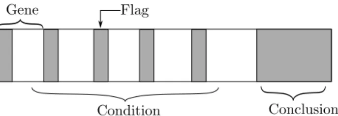
The individuals in these populations represent rules. To allow rules with different lengths, a special encoding is used for the representation of these rules (Figure 8). This fixed length representation, called a chromosome, contains a condition part and a conclusion part. The condition part is subdivided in as many genes as there are input variables. The binary flag in each of these genes indicates whether the conditions on the associated input variable are active or not. When the flag is set to zero, the conditions in the rest of the gene do not apply. The encoding of these conditions is dependent on the type of the input variable the gene is associated with. For example, when the input variable is a binary variable, the rest of the gene is just a zero or one, but if the associated variable is continuous then the rest of the gene consists of an operator and two threshold valuesX1 and X2. The gene can then represent different conditions
such as x < X1 or X1 < x < X2 depending on the value of the operator part.
The gene of the conclusion indicates the class.
mi-PSfrag replacements
Condition Conclusion
Gene Flag
Figure 8: Rule Representation in GEX
gration. Mutation is applied on the chromosomes and randomly changes the information encoded in the genes. Crossover is a gene exchange between two chromosomes and results in two new individuals. Migration is a special oper-ator that transfers weak individuals to a different island. The fitness function to evaluate the rules is based on a weighted average of several aspects such as accuracy, coverage and comprehensibility. By specifying the weights, the ana-lyst can indicate the importance of each of these criteria. Finally, GEX removes those rules that are more specific than other rules or that do not satisfy certain criteria, such as a minimum accuracy or coverage before starting a new iteration. One of the main drawbacks of GEX is the fact that one observation can be covered by multiple rules. Multiple rules can be true for a certain instance and it also not guaranteed that at least one rule will be valid.
The second genetic rule extraction algorithm that is discussed, G-REX
[25, 26] overcomes these problems and delivers exclusive and exhaustive rules. It is also not limited to classification problems. Furthermore, G-REX can pro-duce different types of rules, e.g. decision trees or fuzzy rules. G-REX uses a different representation than GEX to allow the encoding of rules of various length. G-REX is based on a subbranch of genetic algorithms that is called genetic programming and uses S-expressions to represent the individuals. A sample S-expression and its corresponding tree representation are given in Fig-ure 9. Each S-expression contains elements from two sets: a function set and a terminal set. Functions are the internal nodes of the tree and represent op-erations that can be applied on the terminals. The analyst must define these operations and supply the number of arguments that each function can take. The terminals, the leaf nodes in the tree, are the variables and constants from the problem. In the example expression, there are two functions (‘if’ and ‘>’) and 7 terminals (X0,X1, two constants and three class labels).
S-expressions are a powerful alternative to GEX’s flag-mechanism for the encoding of rules or rulesets with varying length. For example, the S-expression of Figure 9 is equivalent to the following ruleset: ‘ifX0 is larger than 27 then
classify as Class 1, else classify as Class 2 ifX1 is larger than 27 and as Class
3 otherwise’. Whereas the above expression is equivalent to a simple decision tree, changing the elements of the terminal and function sets allows different
PSfrag replacements
(if (> X017) Class1 (if(> X1 27) Class2 Class3))
If If Conclusion > > Class 1 Class 2 Class 3 27 17 X0 X1
Figure 9: S-Expression and its corresponding Tree Representation types of rules to be created. The fitness function used to select the fittest indi-viduals is very similar to the one used by GEX and incorporates elements, such as comprehensibility and accuracy.
In [38], an approach was proposed that is very similar to G-REX. The main difference is that artificial examples are used to evaluate the fitness of the rules. The algorithm is outlined in Figure 10. First the setSis initialized: the training observations with the outputs provided by the underlying black box are inserted inS and an initial population of rules is created. The algorithm will then create a user-specified number of artificial examples that are also inserted into the setS. Creation of the artificial examples is performed by taking a training observation and mutating random attribute values. Before inserting the example into S, a check is performed to see if the example is not already present inS and to verify whether the output of the black box for this example is different from the output of the current best rule. If the example passes these checks, it is added intoS. The genetic algorithm will then be executed several times. After this, the correctly classified examples, i.e. examples for which the best rule prediction equals the black box prediction, are removed from S and the entire process is repeated until the algorithm finds rules that are fit enough.
The wide variety of genetic rule extraction algorithms proves that they are a useful tool for the analysis of black box models. The main advantage of these methods is their flexibility to changes. Altering the fitness function al-lows the analyst to select the required accuracy-comprehensibility trade-off and changing the function set even allows the user to change the format of the extracted descriptions. The main drawback of all genetic algorithms are the computational requirements for performing the successive iterations. A second drawback concerns the consistency of the extracted descriptions. Due to the aspect of probability during creation of the rules, we can expect the extracted rules to be significantly different when a genetic algorithm is run several times
1 Initialize the setS
2 Create initial population of rules R 3 While (rules in R are not good enough) 4 Create Examples and Add them to S 5 Evaluate fitness of rules in R
6 Apply genetic programming for N iterations 7 Remove from S the examples for which the output 8 of the ANN equals the output of the best rule 9 End While
Figure 10: Algorithm of Rabu˜nal et al. [38]
on the same data set.
3.2.6 BIO-RE
One of the most straightforward rule extraction algorithms is BIO-RE (Bina-rized Input-Output Rule Extraction) [51]. As suggested by its name, the method is only applicable when all inputs and outputs are binary variables. For other types of variables, a transformation is required. For numerical variables, it is suggested to use the binarization method of Equation 14.
x0
i=
½
1 ifxi ≥µi;
0 otherwise. (14)
withµi the mean value over all xi’s. The idea behind BIO-RE is to create each possible input combination and to query the network for the corresponding output decision. A truth table is generated from the samples and boolean simplification methods are subsequently used to convert this truth table into the corresponding boolean function.
One can observe immediately the disadvantages of this method: because the algorithm first creates all possible input combinations, the method is only applicable when the number of inputs N is small as the number of combinations equals 2N. For many real-word problems this number of combinations is very large, making the method computationally infeasible. The required binarization is also undesirable as it will probably deteriorate classification performance. Because of these two shortcomings, the method seems not applicable to any real-life problem.
3.2.7 BUR
In [10], a pedagogical algorithm for rule extraction, called Boost Unordered Rule Learner (BUR), was proposed. Although BUR was proposed as a rule extraction algorithm for SVM classifiers, it can also be used to learn rules di-rectly form the data points. BUR creates non-exclusive propositional rules and associates with each rule a weight or confidence level. New observations are
classified by finding all rules applicable and combining them such that rules with higher confidence are more important for the final classification decision. BUR incorporates elements from both the rule learner CN2 [11] and ‘gradient boosting machines’[19]. We will first provide a detailed explanation of the ‘gra-dient boosting mechanism’ and afterwards explain how it can be combined with CN2 to perform rule extraction.
Gradient Boosting Machines
In [19], Friedman proposes a method for function estimation coined ‘Gradient Boosting Machines’. Given a set of training observations{xi, yi}N1, the goal of
function estimation is to find a function F*(x) that minimizes a user-defined loss function ψ(y, F(x)). For regression problems, the most widespread loss functions are the squared error and absolute error function.
In [19], Friedman limits the allowed format of the functions F(x) to:
F(x,P) = M
X
m=0
βmh(x;am) (15)
withP={βm,am}M0 a set of parameters. The functionsh(x,am) are called
base learners and are usually chosen to be simple functions ofxwith parameters
a. Possible base learners are single propositional rules, decision trees or linear functions. Friedman refers to several other function approximation methods, such as neural networks and Support Vector Machines, that share the format of Equation 15.
The problem of function estimation can then be formulated as finding the parameters P for which the loss function is minimized:
{βm,am}Mm=0=arg min β0 m,a0m N X i=1 ψ(yi, M X m=0 βm0 h(x;a0m)) (16)
Depending on the loss function and format of the base learners, it might be infeasible to find a solution to this problem and a greedy approach might be required. Starting from an initial approximation F0, the algorithm
itera-tively looks for the best step towards the optimal solution given the current approximation. For m=1,. . . ,M do:
{βm,am}=argmin β,a N X i=1 ψ(yi, Fm−1(xi) +βh(xi;a)) (17) Fm(x) =Fm−1(x) +βmh(x;am) (18) For some loss functions and/or base learners it might be difficult to solve Equation 17 and in those cases gradient descent can be used to find an approx-imate solution.(Appendix A)
AssumingFm−1(x) is the approximation during the m-th iteration, gradient
InitializeF0 For m=1 to M do 1 gm−1(x) = ∂ψ∂F(y,Fmm−1(x)) −1(x) ¯ ¯ ¯x =xi i= 1, . . . , N 2 am= arg mina,βPNi=1(−gm−1(xi)−βh(xi;a))2 3 βm= arg minβPNi=1ψ(yi, Fm−1(xi) +βh(xi;am)) 4 Fm(x) =Fm−1(x) +βmh(x;am) End For
Figure 11: Gradient Boosting
gm−1(x) =
∂ψ(y, Fm−1(x))
∂Fm−1(x)
(19) If gm−1(x) has the same format as the base learners, and in that case can
also be written ash(x,am), then we can find a value forβmby minimizing:
βm=argmin β N X i=1 ψ(yi, Fm−1(xi) +βh(xi;am)) (20)
However,gm−1(x) will usually have a different format than the base learners,
and in that case we will take as h(x,am), the h(x,a) that is most correlated withgm−1(x) over the training data. Therefore,am is the solution of:
am=argmina ,β N X i=1 (−gm−1(xi)−βh(xi;a))2 (21)
A value forβmcan again be obtained from Equation 20. A general overview of the gradient boosting mechanism is given in Figure 11.
Integration with CN2
BUR is based on the above concept of ‘gradient boosting’ and a single proposi-tional rule is chosen as the format of each base learner. Formally,
r(x) =h(x,a) =
+1/−1 if the rule is applicable on examplex
and classifies examples as positive/negative
0 otherwise.
(22) An overview of the basic algorithm is shown in Figure 12. We will explain the differences with Figure 11 below.
The loss function used by BUR is the absolute error function. The calcula-tion ofgm(x) (Step 1 in Figure 11) can therefore be simplified to: