Multivariate Small Area Estimation for Health Indicators

(1)

Research Online

University of Wollongong Thesis Collection

2017+ University of Wollongong Thesis Collections

2017

Multivariate Small Area Estimation for Health Indicators

Mossamet Kamrun Nesa

University of Wollongong

Follow this and additional works at: https://ro.uow.edu.au/theses1

University of Wollongong University of Wollongong

Copyright Warning Copyright Warning

You may print or download ONE copy of this document for the purpose of your own research or study. The University does not authorise you to copy, communicate or otherwise make available electronically to any other person any

copyright material contained on this site.

You are reminded of the following: This work is copyright. Apart from any use permitted under the Copyright Act 1968, no part of this work may be reproduced by any process, nor may any other exclusive right be exercised, without the permission of the author. Copyright owners are entitled to take legal action against persons who infringe

their copyright. A reproduction of material that is protected by copyright may be a copyright infringement. A court may impose penalties and award damages in relation to offences and infringements relating to copyright material.

Higher penalties may apply, and higher damages may be awarded, for offences and infringements involving the conversion of material into digital or electronic form.

Unless otherwise indicated, the views expressed in this thesis are those of the author and do not necessarily Unless otherwise indicated, the views expressed in this thesis are those of the author and do not necessarily represent the views of the University of Wollongong.

represent the views of the University of Wollongong.

Recommended Citation Recommended Citation

Nesa, Mossamet Kamrun, Multivariate Small Area Estimation for Health Indicators, Doctor of Philosophy thesis, School of Mathematics and Applied Statistics, University of Wollongong, 2017.

https://ro.uow.edu.au/theses1/282

Research Online is the open access institutional repository for the University of Wollongong. For further information contact the UOW Library: [email protected]

(2)

Multivariate Small Area Estimation

for Health Indicators

Mossamet Kamrun Nesa

A thesis submitted in fulfillment of the requirements for the award of the degree

Doctor of Philosophy

from

University of Wollongong

(3)

(4)

Doctor of Philosophy

on the topic

Multivariate Small Area Estimation

for Health Indicators

to the

School of Mathematics and Applied Statistics

Faculty of Engineering and Information Sciences

at the University of Wollongong

submitted by

Mossamet Kamrun Nesa

Supervisor:

Assoc. Prof. Robert Clark, PhD (University of Wollongong)

Co-supervisor:

Dr. Carole. L. Birrell, PhD (University of Wollongong)

(5)

I, Mossamet Kamrun Nesa, declare that this thesis, submitted in partial fulfilment of

the requirements for the award of Doctor of Philosophy, in the School of Mathematics

and Applied Statistics, University of Wollongong, is wholly my own work unless

otherwise referenced or acknowledged. The document has not been submitted for

qualifications at any other academic institution.

Mossamet Kamrun Nesa

(6)

(7)

In order to improve the overall health condition of a population, accurate

esti-mates of health indicators are required at a fine spatial scale, such as the

adminis-trative units of a country or regions within a country. Direct estimators tend to have

unacceptably high standard errors for areas with small sample sizes. Model-based

indirect small area estimators borrow strength from related areas and achieve lower

mean squared errors.

The thesis is concerned with multivariate small area estimation (SAE), where

multiple response variables instead of a single response variable are considered

si-multaneously. Two general problems are considered: (1) the use of a multivariate

area level model to get improved estimates for each variable by area and (2) the

estimation of the cross-classification of two or more indicators by area.

The multivariate Fay-Herriot (MFH) model is the natural extension of the widely

used univariate Fay-Herriot (UFH) model where two or more response variables

are considered together. Both numerical and simulation studies are carried out to

investigate under what conditions multivariate small area estimators perform better

than separate univariate estimators. Results show that the MFH model performs

better under some conditions which depend on the values of the parameters such as

(8)

using the MFH model rather than the separate UFH model are greater when the

across-variable correlations of both sampling errors and area level random effects are

high and when the ratio of variances of sampling errors and random effects is high.

A parametric bootstrap approach is developed to allow estimation of mean squared

errors, and confidence intervals for the gain due to multivariate modelling. The

approaches are applied to a 2011/12 New Zealand Health Survey dataset. The MFH

model provides some improvements over UFH model according to mean squared

error estimates of the estimated health indicators by electoral district. However,

wide confidence intervals for the relative efficiencies associated with multivariate

modelling are seen, suggesting that it is difficult in practice to be confident about

gains from multivariate approaches.

A unit level approach for producing small area estimates of cross-classified counts

of two or more indicators is developed, based on a multinomial logit mixed model

with category specific random effects. The application is novel because contingency

tables are modelled in each small area. Other researchers have considered trinomial

data (such as unemployed, employed and inactive counts), whereas we extend these

multinomial methods to allow small area estimation of cross-classified counts. For

example, Obesity byHigh Blood Pressure counts can be estimated for each area in

a health survey. The new method is also different from the well-known existing

Structure Preserving Estimation (SPREE) approach since SPREE combines the

information of auxiliary variables from a previous census with current survey data

to improve the estimators of cells totals in a multi-way contingency table. The mean

(9)

New Zealand Health Survey are used to illustrate the approach.

Small area estimators of cross-classified counts are also developed based on

log-linear models, which are a parsimonious special case of the multinomial logit model.

A number of parsimonious log-linear models are defined and applied to the New

Zealand Health Survey data. These models did not do particularly well on the 2×2 tables considered in the application, but they are more computationally scalable to

three-way and higher order cross-classifications.

Overall, multivariate Fay-Herriot small area estimators are useful in specific

sit-uations which are identified in the thesis, however, it is difficult to be confident with

real data whether one is in such a situation. Multivariate categorical models enable

a new form of small area statistics to be calculated, namely contingency tables of

survey variables by area.

(10)

I would firstly like to express my deep gratitude to my supervisors, Associate

Professor Robert Clark and Dr. Carole Birrell. I am grateful to Robert Clark, for his

encouragement, thoughtful comments, good advice and invaluable patience during

the long journey of my study. Thank you Carole, for your invaluable discussions,

guidance and great enthusiasm.

I would also like to thank Professor Raymond Chambers (University of

Wollon-gong) for his suggestion to develop the ideas of multinomial models.

I would like to acknowledge to University of Wollongong (UOW), Australia,

for the financial support through International Postgraduate Tuition Award and

University Postgraduate Award. Thanks to Shahjalal University of Science and

Technology, Sylhet (SUST), Bangladesh, for sanctioning my study leave to complete

my study.

I would also like to thank to all academic and administrative staffs of National

Institute for Applied Statistics Research Australia (NIASRA) for their support,

encouraging words and cordial assistance.

Thanks to my friends and colleagues particularly Dr. Chandra Gulati, Dr.

Payam Mokhtarian, Dr. Bothaina Bukhatwa, Dr. Nawa and Dr. Sumonkanti Das

(11)

I am grateful to my parents and family for their support and commitment to

my education. Special thanks to my sisters Tumpa, Rupa and Pinky to take care of

my son during my second year of PhD and Nipu for her appreciable encouragement.

Thanks to Mr.Niru and Mrs.Runa for a great financial support at the very beginning

of my PhD.

I am very much thankful to my husband Mohammad Tareq Mamun Khan, for his

unfailing love, patience, support and encouragement. Most importantly, thanks to

my son Rahil Sarbi Khan, for his unconditional love, patience and sacrifice during the

journey of my PhD. Thanks baba (Sarbi) for encouraging me through the dialogue

“Mum don’t read the newspaper, do your work. You have to finish your PhD”.

(12)

1 Introduction 1

1.1 The Definition and Relevance of Small Area Estimation . . . 1

1.2 Multivariate Small Area Estimation . . . 3

1.3 Area Level Models . . . 4

1.4 Unit Level Models . . . 6

1.5 Structure of the Thesis . . . 8

2 Literature Review 11 2.1 Notation and Definitions . . . 12

2.2 Direct Estimators . . . 14

2.2.1 Design-Based Direct Estimators . . . 14

2.2.2 Model-Assisted Direct Estimators . . . 16

2.2.3 Model-Based Direct Estimators . . . 19

2.3 Indirect Small Area Estimation . . . 20

2.3.1 Synthetic Estimators . . . 20

2.3.2 Composite Estimators . . . 21

(13)

Level Models . . . 22

2.5 Small Area Estimation: Multivariate Area Level Models . . . 27

2.6 Small Area Estimation: Univariate Unit Level Models . . . 32

2.7 Small Area Estimation of a Single Classifications . . . 41

2.8 Structure Preserving Estimation Model . . . 45

3 Theoretical and Numerical Evaluation of Bivariate Fay-Herriot Model 48 3.1 Introduction . . . 48

3.2 Approximate Theoretical Relative Efficiency of Bivariate Fay-Herriot Compared to Univariate Fay-Herriot Model . . . 50

3.3 Special Cases . . . 55

3.4 Numerical Study . . . 57

3.4.1 Setting the Parameters . . . 58

3.4.2 Descriptive Summary of Numerical Study . . . 60

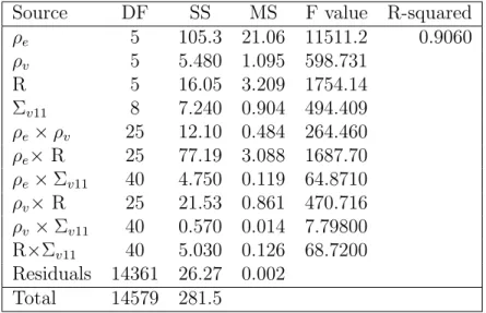
3.4.3 Formal Analysis of Numerical Study: Analysis of Variance . . 68

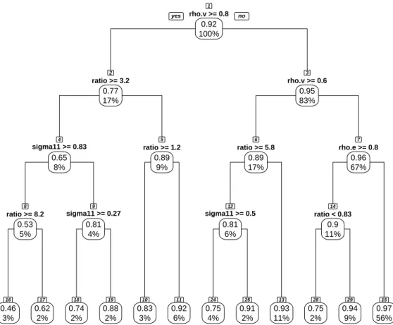
3.4.4 Formal Analysis of Numerical Study: Regression Tree . . . 71

3.5 Simulation Experiment . . . 76

3.5.1 Design of the Experiment . . . 76

3.5.2 Results of the Simulation Experiment . . . 78

(14)

4 MSE Estimation and Empirical Study for Bivariate Fay-Herriot

Model 83

4.1 Introduction . . . 83

4.2 Example Dataset: The New Zealand Health Survey . . . 85

4.2.1 Sample Design . . . 86

4.2.2 Data Variables . . . 87

4.2.3 Sampling Variance Calculation . . . 89

4.3 Methodology . . . 91

4.3.1 Model Fitting via Maximum Likelihood Estimation . . . 91

4.3.2 Parametric Bootstrap Mean Squared Error . . . 92

4.4 New Zealand Health Survey Data Analysis . . . 94

4.4.1 Results for One Pair of Variables . . . 94

4.4.2 Results for All Pairs of Variables . . . 96

4.5 Bootstrap Confidence Intervals for the Relative Efficiency . . . 99

4.5.1 Parametric Bootstrap Confidence Interval . . . 100

4.5.2 Application to New Zealand Health Survey Data . . . 101

4.5.3 Application to Simulated Data . . . 103

4.6 Summary . . . 104

5 Estimating Small Area Contingency Tables using Multinomial Mod-els 106 5.1 Introduction . . . 107

5.2 Multinomial Model for Cross-Classified Data . . . 110

(15)

5.2.2 Binomial Case . . . 112

5.2.3 Fournomial Case . . . 113

5.3 Maximum Likelihood Estimation of Parameters . . . 116

5.3.1 Calculation of the Likelihood . . . 116

5.3.2 Maximization of the Likelihood . . . 118

5.3.3 Prediction of uˆd . . . 119

5.3.4 Prediction of ˆpdr using ˆudr . . . 120

5.4 Mean Squared Error Estimation using a Parametric Bootstrap . . . 122

5.5 Multinomial Modelling in Complex Survey Design . . . 123

5.6 Outline of the Empirical Study . . . 125

5.7 Results for Obesity byHigh Blood Pressure . . . 126

5.7.1 Fitted Model for Obesity byHigh Blood Pressure . . . 126

5.7.2 Small Area Estimates and Corresponding RMSEs of Obesity byHigh Blood Pressure Contingency Tables . . . 129

5.7.3 Small Area Estimates and Corresponding RMSEs of Marginal Prevalences ofObesity and High Blood Pressure . . . 131

5.8 Results for Current Smoker byObesity . . . 135

5.8.1 Fitted Model for Current Smoker by Obesity . . . 135

(16)

Smoker by Obesity Contingency Tables . . . 138

5.8.3 Small Area Estimates and Corresponding RMSEs of Marginal Prevalences ofCurrent Smoker and Obesity . . . 140

5.9 Summary . . . 144

6 Estimating Small Area Contingency Tables using Log-linear Mod-els 146 6.1 Introduction . . . 146

6.2 Log-linear Models for Cross-Classified Data . . . 149

6.2.1 Definition of the Model . . . 149

6.2.2 Constraints and Estimation of Parameters for 2×2 Tables . . . 151

6.3 The Relationship Between Multinomial and Log-linear Models for 2×2 Tables . . . 153

6.4 Model Simplification . . . 156

6.5 Maximum Likelihood Estimation of Parameters . . . 160

6.6 Outline of the Empirical Study . . . 161

6.7 Results of Empirical Study . . . 162

6.7.1 Maximum Likelihood Parameter Estimates . . . 162

6.7.2 Small Area Estimates and Corresponding RMSEs of Current Smoker by Obesity Contingency Tables . . . 163

(17)

Prevalences ofCurrent Smoker and Obesity . . . 165

6.7.4 Model Comparison . . . 168

6.8 Simulation Experiment . . . 169

6.9 Results of Simulation Experiment . . . 174

6.9.1 Absolute Relative Bias for 2×2 Tables . . . 174

6.9.2 Absolute Relative Bias of Marginal Prevalences . . . 179

6.9.3 Relative Efficiency for 2×2 Tables . . . 182

6.9.4 Relative Efficiency of Marginal Prevalences . . . 186

6.10 Summary . . . 189

7 Conclusion 191 7.1 Summary and Conclusions . . . 191

7.2 Future Research . . . 197

A Derivations for Chapter 3 202 A.1 BLUP and MSE for UFH Estimator when Regression Parameter βis Known . . . 202

A.2 Log Likelihood for UFH Estimator . . . 207

A.3 BLUP and MSE for BFH Estimator when Regression Parameter βis Known . . . 207

A.4 Log Likelihood for BFH Estimator . . . 215

A.5 Relative Efficiency . . . 216

A.6 Special Cases . . . 216

(18)

A.6.2 Case 3 . . . 219

A.6.3 Case 4 . . . 220

A.6.4 Case 5 . . . 223

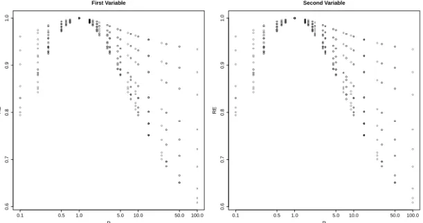
A.7 The Effects of R Ratio on Relative Efficiency . . . 228

B Additional Calculations for Chapter 4 234 B.1 Sampling Variance Calculation . . . 234

B.2 New Zealand Health Survey Data Analysis . . . 235

B.2.1 Results for One Pair of Variables . . . 235

B.2.2 Results for All Pairs of Variables . . . 237

C Additional Graphs for Chapter 5 240 C.1 Results . . . 240

C.1.1 Small Area Estimates and Corresponding RMSEs of Marginal Prevalences ofObesity and High Blood Pressure . . . 240

C.1.2 Small Area Estimates and Corresponding RMSEs of Marginal Prevalences ofCurrent Smoker and Obesity . . . 242

D Additional Tables for Chapter 6 244 D.1 Tables for Absolute Relative Bias . . . 245

D.2 Tables for Relative Efficiency . . . 256

Bibliography 261

(19)

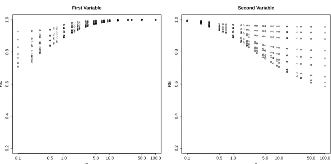
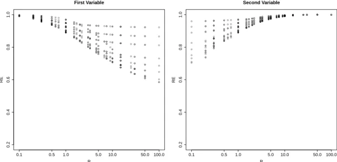
3.1 Results of relative efficiency, RE, defined in (3.16) for the first and

second variables with different values of ρv. . . 62

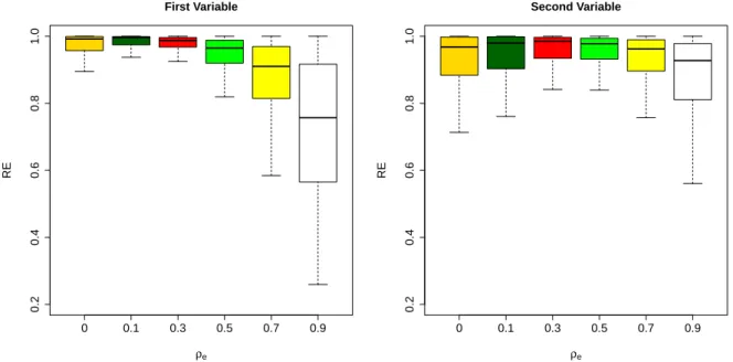
3.2 Results of relative efficiency, RE, defined in (3.16) for the first and

second variables with different values of ρe. . . 62

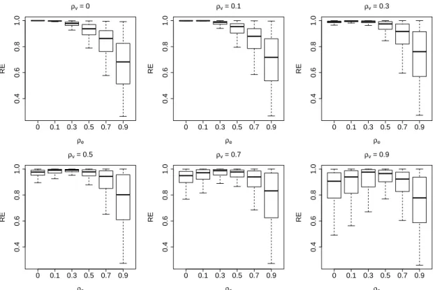
3.3 Results of relative efficiency, RE, defined in (3.16) with constant ρv

and different values ofρe for the first variable. . . 63

3.4 Results of relative efficiency, RE, defined in (3.16) with constant ρv

and different values ofρe for the second variable. . . 63

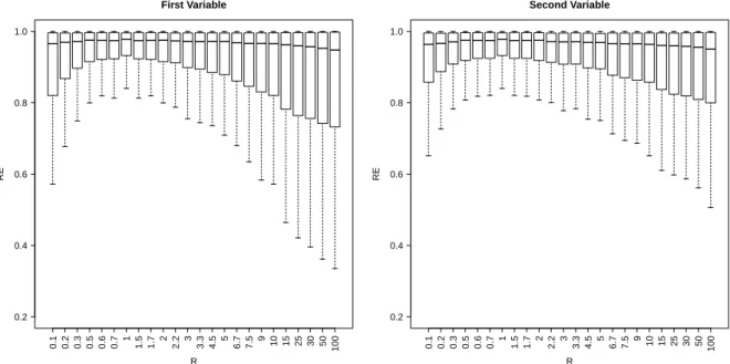
3.5 Results of relative efficiency, RE, defined in (3.16) against ratio, R=re

rv. 65

3.6 Results of relative efficiency, RE, defined in (3.16) against ratio,

R=re

rv, with ρv =ρe = 0.7. . . 66

R=re

rv, with ρv = 0.7,ρe = 0.1. . . 67

R=re

rv, with ρv = 0.1, ρe = 0.7. . . 68

3.9 Histogram of standardized residuals. . . 69

3.10 Regression tree for predicting relative efficiency (First variable). . . . 74

(20)

4.1 Distribution of area-specific sample sizes. . . 90

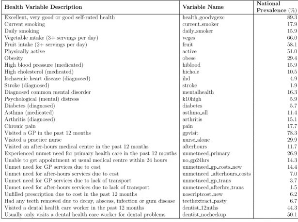
4.2 Distribution of the estimated relative root mean squared errors

(RRM-SEs%) across 63 areas forObesity(left panel) andHigh Blood Pressure

(right panel) for the direct, UFH and BFH estimators. . . 96

4.3 Distribution of the estimated median relative root mean squared

er-rors (RRMSEs%) of the direct, UFH and BFH estimates over 63 areas

for 870 ordered pairs of indicator variables. . . 98

4.4 Distribution of the estimated median relative efficiencies (REs) of

the BFH and UFH estimators relative to the direct estimators over

63 areas for 870 values of indicator variables. . . 98

4.5 Distribution of the quartiles of the relative efficiencies (REs) of BFH

relative to UFH estimators over areas based on 870 ordered pairs of

indicator variables. . . 99

4.6 Distribution of the minimum relative efficiencies (REs) of BFH

rel-ative to UFH estimators over areas based on 870 ordered pairs of

indicator variables. . . 99

4.7 Confidence Interval of the relative efficiencies (REs) of BFH over 63

areas forObesity andHigh Blood Pressure estimates. LL=Lower

Con-fidence Limit, ER=Estimated RE and UL=Upper ConCon-fidence Limit. . 102

(21)

63 areas for 870 ordered pairs of indicator variables. LL=Lower

Con-fidence Limit, ER=Estimated RE and UL=Upper ConCon-fidence Limit. . 102

4.9 Boxplots of the LL, ER and UL from the 95% Confidence Intervals

of relative efficiencies (REs) over 100 areas when ρe = 0.5 and wd=

1. LL=Lower Confidence Limit, ER=Estimated RE and UL=Upper

Confidence Limit. . . 104

5.1 Distribution of the direct estimates of Obesity prevalence by High

Blood Pressure prevalence in percentages across 63 general election

districts. . . 128

5.2 Small area estimates (SAEs) based on the fournomial model versus

the direct estimates of cells of the contingency table of Obesity by

High Blood Pressure . . . 130

5.3 Distribution of estimated root mean squared errors (RMSEs%) of the

direct and the fournomial estimators of cells of the contingency table

of Obesity byHigh Blood Pressure across the general election districts 131

5.4 Small area estimates (SAEs) based on the the binomial model and

the fournomial model versus the direct estimates of the marginal

pro-portions of Obesity and High Blood Pressure . . . 133

5.5 Distribution of root mean squared errors (RMSEs%) of the direct,

UFH, binomial and fournomial marginal estimators of Obesity and

High Blood Pressure across the general election districts. . . 134

(22)

binomial and fournomial marginal estimators of Obesity and High

Blood Pressure against sample size. . . 134

5.7 Distribution of the direct estimates ofCurrent Smoker prevalence by

Obesity prevalence in percentages across 63 general election districts. 136

5.8 Small area estimates (SAEs) based on the fournomial model

ver-sus the direct estimates of cells of the contingency table of Current

Smoker by Obesity . . . 139

5.9 Distribution of estimated root mean squared errors (RMSEs%) of the

direct and the fournomial estimators of cells of the contingency table

of Current Smoker by Obesity across the general election districts . . 140

5.10 Small area estimates (SAEs) based on the binomial model and the

fournomial model versus the direct estimates of the marginal

propor-tions of Current Smoker (CS) and Obesity (OBS) where the point

size is proportional to sample size . . . 142

5.11 Distribution of root mean squared errors (RMSEs%) of the direct,

binomial and fournomial marginal estimators ofCurrent Smoker and

Obesity across the general election districts. . . 143

5.12 Plots of root mean squared errors (RMSEs%) of the direct, binomial

and fournomial marginal estimators of Current Smoker and Obesity

against sample size. . . 143

(23)

(saturated and three non-saturated log-linear models) and direct

es-timates of the prevalence of each cell of Current Smoker and Obesity 164

6.2 Distribution of root mean squared errors (RMSEs%) of the four

log-linear estimators of the prevalences of Current Smoker by Obesity

across the general election districts . . . 165

6.3 Difference between small area estimates (SAEs) and direct estimates

based on the binomial, saturated and other log-linear models (Model

1-Model 3) of the marginal proportions ofCurrent Smoker andObesity166

6.4 Distribution of root mean squared errors (RMSEs%) of the binomial,

saturated and other log-linear (Model 1-Model 3) marginal estimators

of Current Smoker and Obesity across the general election districts. . 166

6.5 Area averages of absolute relative biases (ARBs%) of the saturated

model versus direct estimator for each cell for 48 combinations . . . . 175

model versus Model 1 for each cell for 48 combinations . . . 176

model versus Model 2 for each cell across 48 combinations . . . 177

model versus Model 3 for each cell for 48 combinations . . . 178

6.9 Area averages of absolute relative biases (ARBs%) of marginal

esti-mates of the saturated model versus direct estimators for 48

combi-nations. . . 179

(24)

mates of the saturated model versus binomial model for 48

combina-tions. . . 180

esti-mates of the saturated model versus Model 1 for 48 combinations. . . 180

6.14 Results of relative efficiencies (REs) of the saturated model and Model

1 for each cell for 48 combinations . . . 183

6.17 Results of relative efficiencies (REs) of marginal estimates of the

sat-urated model and binomial model for 48 combinations. . . 186

sat-urated model and Model 1 for 48 combinations. . . 187

(25)

R=re

rv, with ρv =ρe = 0.1. . . 228

A.2 Results of relative efficiency, RE, defined in (3.16) against ratio,

R=re

rv, with ρv =ρe = 0.5 . . . 230

A.3 Results of relative efficiency, RE, defined in (3.16) against ratio, R=re

rv

with ρv =ρe = 0.9 . . . 230

R=re

rv, with ρv = 0.5, ρe = 0.7. . . 231

R=re

rv, with ρv = 0.7, ρe = 0.5. . . 231

R=re

rv, with ρv = 0.9, ρe = 0.1. . . 232

R=re

rv, with ρv = 0.1, ρe = 0.9. . . 232

R=re

rv, with ρv = 0.9, ρe = 0.5. . . 233

R=re

rv, with ρv = 0.5, ρe = 0.9. . . 233

B.1 Distribution of the estimated relative root mean squared errors

(RRM-SEs%) across 63 areas forObesity(left panel) andHigh Blood Pressure

(right panel) for the direct, UFH and BFH estimators. . . 237

(26)

rors (RRMSEs%) of the direct, UFH and BFH estimates over 63 areas

for 870 ordered pairs of indicator variables. . . 238

B.3 Distribution of the estimated median relative efficiencies (REs) of

the BFH and UFH estimators relative to the direct estimators over

63 areas for 870 values of indicator variables. . . 239

C.1 Distribution of root mean squared errors (RMSEs%) of the direct,

UFH, binomial and fournomial marginal estimators of Obesity and

High Blood Pressure across the general election districts. . . 241

C.2 Plots of root mean squared errors (RMSEs%) of the direct, UFH,

binomial and fournomial marginal estimators of Obesity and High

Blood Pressure against sample size. . . 241

C.3 Distribution of root mean squared errors (RMSEs%) of the direct,

UFH, binomial and fournomial marginal estimators ofCurrent Smoker

and Obesity across the general election districts. . . 243

C.4 Plots of root mean squared errors (RMSEs%) of the direct, UFH,

binomial and fournomial marginal estimators ofCurrent Smoker and

Obesity against sample size. . . 243

(27)

3.1 Values of parameters . . . 59

3.2 Analysis of variance (ANOVA) on relative efficiency of the first

vari-able, for up to two-way interactions . . . 70

3.3 Analysis of variance (ANOVA) on relative efficiency of the second

variable, for up to two-way interactions . . . 71

3.4 Summary table of lower relative efficiency (RE) of the first variable

from Figure 3.10 . . . 76

3.5 Summary table of lower relative efficiency (RE) of the second variable

from Figure 3.11 . . . 76

3.6 Medians of RE over D= 100 small areas with wd = 1 . . . 79

3.7 Medians of RE over D= 100 small areas with wd =

p

Z2

d1+Z

2

d2 . . . 79

4.1 Description of the key indicators in the NZHS dataset . . . 89

4.2 Description of the covariates (Z) used in the Fay-Herriot models for

the NZHS dataset . . . 89

4.3 Estimates and 95% CIs of the elements ofΣv . . . 94

(28)

ρe = 0.5 and wd = 1. LL is the lower confidence limit, ER is the

estimated relative efficiency and UL is the upper confidence limit . . 104

5.1 Notation for joint and marginal probabilities . . . 108

5.2 Five number summary and mean of population size (Nd), sample size

(md) and effective sample size (m∗d) of general election districts in

2011/12 NZHS . . . 126

5.3 Five number summary and mean of direct estimates of the prevalence

of Obesity (OBS) and prevalence of High Blood Pressure (HBP) in

percentage across the general election districts . . . 127

5.4 National prevalences (in percentages) of Obesity prevalence by High

Blood Pressure prevalence . . . 127

5.5 Five number summary and mean of small area estimates (proportions)

and root mean squared errors (RMSEs%) estimates based on direct,

binomial and fournomial marginal proportions ofObesity (OBS) and

High Blood Pressure (HBP) . . . 135

5.6 Five number summary and mean of direct estimates of the

preva-lence of Current Smoker (CS) and prevalence of Obesity (OBS) in

percentage across the general election districts . . . 136

5.7 National prevalences in percentage of Current Smoker by Obesity . . 136

(29)

and root mean squared errors (RMSEs%) estimates based on direct,

binomial and fournomial marginal proportion ofCurrent Smoker (CS)

and Obesity (OBS) . . . 144

6.1 Coefficient of variation (CV) of the prevalences of Current Smoker

(CS), Obesity (OBS) and odds ratio (OR) under fitted model . . . 163

6.2 Five number summary of small area estimates of marginal proportion

of Current Smoker (CS) and Obesity (OBS) based on the binomial,

saturated, and Model 1 to Model 3 . . . 167

6.3 Five number summary of root mean squared errors in percentage

of marginal proportion of Current Smoker (CS) and Obesity (OBS)

based on the binomial, saturated, and Model 1 to Model 3 . . . 167

6.4 Akaike Information Criterion (AIC) and Bayesian Information

Crite-rion (BIC) of log-linear models relative to Model 2 . . . 168

6.5 Design of parameters options. Each row defines an option for a

pa-rameter or vector of papa-rameters . . . 171

6.6 Combinations of parameters . . . 173

B.1 Estimates and 95% CIs of the elements of Σv . . . 235

D.1 Area averages of absolute relative biases (ARBs%) of the direct,

sat-urated and non-satsat-urated log-linear models for panel (a) (prevalence

of Y1 = 1 andY2 = 0) . . . 245

(30)

urated and non-saturated log-linear models for panel (b) (prevalence

of Y1 = 0 andY2 = 1) . . . 246

sat-urated and non-satsat-urated log-linear models for panel (c) (prevalence

of Y1 = 1 andY2 = 1) . . . 247

sat-urated and non-satsat-urated log-linear models for panel (d) (prevalence

of Y1 = 0 andY2 = 0) . . . 248

D.5 Absolute biases and root mean squared errors (RMSEs) of the direct

and the saturated model in percentage for panel (a) (prevalence of

Y1 = 1 andY2 = 0) . . . 249

and the saturated model in percentage for panel (b) (prevalence of

Y1 = 0 andY2 = 1) . . . 250

and the saturated model in percentage for panel (c) (prevalence of

Y1 = 1 andY2 = 1) . . . 251

and the saturated model in percentage for panel (d) (prevalence of

Y1 = 0 andY2 = 0) . . . 252

(31)

proportion of the first variable (1st var) and the second variable (2nd

var) under the direct, binomial, fournomial and log-linear models. . . 253

D.10 Absolute biases and root mean squared errors (RMSEs) of the marginal

estimators of direct and saturated model in percentage for the first

variable . . . 254

D.11 Absolute biases and root mean squared errors (RMSEs) of the marginal

estimators of direct and saturated model in percentage for the second

variable . . . 255

D.12 Relative efficiencies of the saturated and non-saturated log-linear

models for panel (a) (prevalence of Y1 = 1 and Y2 = 0) . . . 256

models for panel (b) (prevalence of Y1 = 0 and Y2 = 1) . . . 257

models for panel (c) (prevalence of Y1 = 1 and Y2 = 1) . . . 258

models for panel (d) (prevalence of Y1 = 0 and Y2 = 0) . . . 259

D.16 Relative efficiencies of the marginal prevalences of binomial, fournomial

and log-linear models for the first variable (1st var) and the second

variable (2nd var) . . . 260

(32)

AIC Akaike Information Criterion

ANOVA Analysis of variance

ARB Absolute relative bias

BFH Bivariate Fay-Herriot

BIC Bayesian Information Criterion

BLUP Best linear unbiased prediction

CART Classification and Regression Tree

CI Confidence Interval

CV Coefficient of variation

EBLUP Empirical best linear unbiased prediction

FH Fay-Herriot

GED General election districts

GLMM Generalized linear mixed model

MFH Multivariate Fay-Herriot

ML Maximum likelihood

MSE Mean squared error

NZHS New Zealand Health Survey

(33)

RE Relative efficiency

RMSE Root mean squared error

RRMSE Relative root mean squared error

SAE Small area estimation

SPREE Structure Preserving Estimation

UFH Univariate Fay-Herriot

(34)

Introduction

1.1 The Definition and Relevance of Small Area

Estimation

Trustworthy official statistics on small area level are indispensable indicators of the

social, economic and business conditions of the country. Typically, such small areas

are the micro-level administrative units of a country or a state. Such area estimates

provide information for policy making, regional planning, micro and macro economic

management, labour market research, public health research and evaluation of public

policies.

Survey data are now widely used to provide estimates not only for the total

population but also for subpopulations (also known as domains). Domains can

be defined by geographic areas or sociodemographic groups or cross classification

of both. For example, a geographic domain may incorporate a state or province,

municipality, country, metropolitan area, and socio-demographic domains may be

defined by sex and age group, possibly within a large geographic area (Rao and

Molina, 2015, p.1). A domain or area is known as large when the domain-specific

sample size is large. Domains or area estimators that are obtained based only on

(35)

the sample data from the domain or area are known as direct estimators. Direct

estimation methods such as the design-based Horvitz-Thompson estimator (HT)

(Horvitz and Thompson, 1952) or the model-assisted generalized regression (GREG)

estimator (S¨arndal et al., 1992) are effective when the domain-specific sample sizes

are large. However, in practice, when the domain-specific sample sizes are not

large enough (known as small areas), sufficiently precise direct estimates cannot be

produced. In such situations, small area estimation (SAE) methods can be used to

get reliable estimates of the parameters of interest from related areas.

Indirect SAE estimators that “borrow strength” from sampled observations of

other areas through appropriate linking models are often necessary to produce small

area estimates with an adequate level of precision. Indirect estimators, for example,

synthetic and composite estimators, provide better precision than direct estimators.

Synthetic estimators for small areas are derived under the assumption that small

areas have the same characteristics (in some sense) as larger areas that contain them

(Chambers and Clark, 2012, p.162). Composite estimators are weighted averages of

direct estimators and synthetic estimators (Rao and Molina, 2015, p.57). However,

both of these estimators suffer from design-bias, which does not necessarily decrease

as the sample size increases.

Model-based small area estimation methods “borrow strength” from other areas

of population for estimating small area statistics (for example, means, totals,

propor-tions). Some SAE techniques make use of mixed models by incorporating random

effects. The random effects account for the between area variation that cannot be

(36)

on either area level or unit level models on the basis of data availability. When unit

level data are inaccessible, area level models are developed using direct area-specific

estimates available from a survey dataset and area level covariates available from a

census or administrative dataset.

Many researchers have investigated the application of area level models through

modelling one response variable on area-specific covariates, see for example Prasad

and Rao (1990), Rao (2003a). However, it may be desirable to consider multiple

dependent variables together. The focus of this thesis is on small area estimation

with multiple dependent variables.

1.2 Multivariate Small Area Estimation

This thesis will develop SAE methods considering two or more correlated response

variables together and apply the developed methodologies to health indicators on a

New Zealand Health Survey (NZHS) dataset. The main aims of this thesis are:

• to develop an area level multivariate model for multiple response variables where multiple health indicators are considered together as response variables;

• to develop a unit level approach based on multinomial logit mixed models for multiple-category response variables to produce small area estimates of

cross-classified counts of two or more health indicators by area;

• to simplify the multinomial logit mixed model using log-linear models, which will make higher order contingency tables feasible; and

(37)

• to implement the developed methodologies using health indicators in the NZHS data for examining the performances of the developed methods.

1.3 Area Level Models

The most widely used area level model in SAE is the Fay-Herriot (FH) model (Fay

and Herriot, 1979). It was used first to estimate mean per capita income for small

areas in the USA. In the univariate Fay-Herriot model (UFH), the direct survey

estimates of a single response variable in each area are regressed on area-specific

covariates obtained from census data. For example, suppose a survey is designed

to estimate per capita income. Estimates of per capita income might be obtained

with adequate precision at the country level. However, to obtain estimates for

districts, if the sample sizes are very small then the variances of the estimates will

be high. In order to improve the precision of these estimates, the area (districts)

level direct estimates are regressed on area level covariates obtained from census or

administrative data sources (Fay and Herriot, 1979).

The area level FH model is one of the most popular methods used in SAE because

of its flexibility in combining and explaining different sources of information. Also

it does not require unit level data. Various extensions of the basic area level model

have been proposed to handle correlated sampling errors, spatial dependence of the

model errors, time series and cross-sectional data (Rao and Molina, 2015, pp.83-87).

Statisticians use the UFH model for one variable or separately for each variable.

However, in some surveys it may be desirable to consider two or more correlated

(38)

can be used to incorporate the correlation among the response variables. When

mul-tiple dependent variables are correlated, MFH models may produce better results

than UFH models, but these models have received relatively little attention. There

is limited work on the benefits of MFH models. Datta et al. (1998) compared the

precision of small area estimators obtained from UFH and MFH models, showing

that more precise SAEs are obtainable using MFH models rather than using separate

UFH models for each variable. Gonz´alez-Manteigaet al.(2008) studied MFH models

with constant random effects for each variable and compared an analytic estimator

of mean squared error (MSE) with the bootstrap mean squared error estimator, and

showed that the bootstrap estimator provided lower MSEs than the analytic

estima-tor. Gonz´alez-Manteiga et al.(2008) also described a simulation study designed for

comparing MFH and UFH estimators, and concluded that multivariate modelling

reduced the MSE of the SAE estimators.

One of the focuses of this thesis is to elucidate conditions under which MFH

models work better than separate UFH models based on an approximation of MSE.

This will be investigated both theoretically and numerically for a wide range of

scenarios. The efficiency of MFH and UFH estimators are also investigated via a

simulation study following that of Gonz´alez-Manteiga et al. (2008).

In addition, a parametric bootstrap method of calculating MSE is developed

and applied to the NZHS dataset. The efficiencies of UFH and MFH estimators are

(39)

1.4 Unit Level Models

In the basic unit level model, unit values of the single response variable are regressed

on unit-specific auxiliary variables through a nested error linear regression model.

For instance, a survey may be designed to estimate the total wages and salaries of

workers. Let the survey be designed in such a way that the estimates with desired

precision are possible at the total level. If the interest is to estimate total wages

and salaries at the industry level, then the sample sizes of the industries may be

too small to obtain adequate error variances. In such a situation, auxiliary variables

such as gross business income from firm-level can be used to fit a linear mixed model

considering industry-specific random effects in order to improve the precision of the

estimates (Rao, 2003a). An earlier development of the idea of a unit level model

can be found in Battese et al. (1988) where the nested error regression model was

used to estimate the country crop areas using sample survey data in the USA. They

also used unit level auxiliary variables in their model. This type of unit level model

is appropriate for continuous response variables.

In addition, various extensions of the basic unit level model have been

consid-ered to handle binary responses (Rao and Molina, 2015, pp.88-91). For example,

generalized linear mixed models (GLMM) are used when the response variables are

binary or count values. MacGibbon and Tomberlin (1987) used a logistic regression

model with random area-specific effects to estimate the small area proportions of

binary response variables with unit level auxiliary variables. Unit level data, which

(40)

happen to all be at the area level. A number of studies have used multinomial logit

mixed models to estimate the small area population counts that are classified by a

single survey variable (e.g. labour force status) (Molinaet al., 2007, Saei and Taylor,

2012, L´opez-Vizca´ıno et al., 2013) but not for small area counts cross-classified by

multiple survey variables.

With a multi-category response variable (e.g. labour force status), GLMMs must

be used rather than linear mixed models since the variable of interest is discrete (Rao

and Molina, 2015, p.93). For example, Molina et al. (2007) estimated labour force

characteristics by small areas in the United Kingdom (UK) using a multinomial logit

mixed model with constant random effects for each category. Saei and Taylor (2012)

also proposed a multinomial logit mixed model with category-specific random effects

in estimating labour force status in the UK, showing that the multinomial models

with category-specific area random effects lead to better SAEs than models with

constant random effects for each category.

This thesis will consider estimating small area cross-classified counts of two

bi-nary health indicators, such as counts of Obesity by High Blood Pressure. A

multi-nomial logit mixed model with category-specific area random effects will be used to

estimate the population cell counts by area. This idea is one of the methodological

innovations compared to the existing literature since counts in contingency tables

are modelled in each small area rather than considering the trinomial data (such

as unemployed, employed and inactive counts). This idea can provide small area

estimates of cross-classification of multiple binary variables instead of separately

(41)

by Zhang and Chambers (2004) is an existing approach to estimating small area

cross-classified counts of response variables based on survey data where the

corre-sponding auxiliary information may come from a previous census. The proposed

method of estimating contingency table is different from the SPREE approach as it

considers the cross-classification of target variables from the current survey rather

than combining small area classifications from a previous census with

cross-classifications of target variables of current survey data.

Another contribution set out in this thesis is the development of log-linear

mod-els with category-specific random effects. These are a flexible way of simplifying

multinomial logit mixed models to obtain small area estimates of cross-classified

counts. Log-linear models will allow small area estimates of two-way and higher

order cross-classifications of response variables for each small area. To estimate the

MSE under the mixed multinomial and log-linear models, a parametric bootstrap

method is developed and data from the NZHS are used to illustrate the approach.

Moreover, a simulation study is also conducted for investigating the performance of

multinomial and log-linear models.

1.5 Structure of the Thesis

This thesis considers multivariate small area estimation with multiple continuous

and categorical response variables instead of a single response variable. In Chapter

3 and 4, the multivariate area level model is used to get estimates of each continuous

variable by area; and in Chapter 5 and 6, the estimation of the cross-classification

(42)

Chapter 2 summarizes the main literature relevant to this thesis, comprising

design-based, model-assisted and model-based estimation methods including

uni-variate and multiuni-variate Fay-Herriot models. The review also covers SAE methods

for estimating small area population counts that are cross-classified. The

multino-mial and log-linear models are also reviewed.

Chapter 3 compares the efficiency of SAEs from UFH and MFH models from both

theoretical and numerical perspectives. Expressions for the approximate relative

ef-ficiency for some special cases are derived to give insights into the circumstances

under which the MFH model provides gains over the UFH model. A numerical and

a simulation study of MFH estimation are carried out in this chapter. The numerical

study is conducted to investigate the question of whether, and under what

condi-tions, the MFH model is advantageous compared with the UFH model in small area

estimation. This is accomplished by calculating the approximate MSEs from UFH

and MFH models for a range of model parameter values. An analysis of variance

(ANOVA) approach and a regression tree approach are used to summarize the

re-sults of the numerical study. This chapter also includes a simulation study following

Gonz´alez-Manteiga et al. (2008), assuming known parameters for generating data,

to illustrate the efficiency of the MFH estimators compared to that of the UFH

estimators.

In Chapter 4, an empirical study is conducted using the New Zealand Health

Survey data. A parametric bootstrap method is used to estimate the MSE and the

estimated MSEs of the MFH and UFH SAEs are compared. In addition, parametric

(43)

calculated to assess the uncertainty around the gain of MFH over UFH.

Chapter 5 develops methods for estimating small area cross-classified counts and

the methods are assessed using the NZHS dataset. This chapter uses a

multino-mial logit mixed model to estimate small area cross-classified counts with

category-specific random effects. For example, cross-classified counts by Current Smoker by

Obesity, which constitutes a 2×2 contingency table, are estimated. Estimates of marginal prevalences are also calculated using the multinomial logit mixed model.

In addition, mean-squared errors of the estimates are calculated using a parametric

bootstrap method.

Chapter 6 defines a saturated mixed log-linear model which is equivalent to

the multinomial logit mixed model of Chapter 5. Three non-saturated log-linear

models are also developed by dropping out some parameters from the saturated

log-linear model. The efficiency of SAEs from the saturated model are compared

to those from the three non-saturated log-linear models through an empirical and

a simulation study. In the empirical study, the methods are evaluated using the

NZHS dataset to calculate SAE estimates from two-way contingency tables.

Log-linear models developed in this chapter are more parsimonious than the multinomial

model, which would be particularly important in the estimation of third or higher

order contingency tables by area.

Chapter 7 provides a summary of the major findings of this thesis and suggestions

for future research. Appendices contain proofs of all theoretical results which are

(44)

Literature Review

The term small area or small domain is commonly used to describe small

geographi-cal areas of a country or domains of a population. Classic examples of small areas or

small domains include geographical classifications such as states, countries, districts

or municipalities and subgroups such as specific races or ages in a population (Jiang

et al., 2002).

Small area estimation (SAE) methods are widely used to estimate population

parameters for targeted areas or domains with small sample size. In such situations,

direct estimates which rely on domain-specific surveyed observations may have large

sampling variance (Rao, 2003b, p.1) and indirect estimation methods are therefore

necessary in order to achieve an adequate level of precision. Design-based estimators

are examples of direct estimators, while model-based estimators may be direct or

indirect estimators. Indirect estimators based on a model borrow strength by using

observations of the variable of interest from other areas or time periods in order to

increase the effective sample size in the area and thus decrease the standard errors

(Chambers and Clark, 2012, p.162). Furthermore, auxiliary information is vital for

small area estimation because the most elaborate model cannot work properly if it

(45)

does not involve a set of covariates with good predictive power for the small area

quantities of interest (Pfeffermann, 2013).

The review in this chapter covers both design-based and model-based methods of

small area estimation. After defining the notation to be used in this thesis in Section

2.1, design-based, model-assisted and model-based direct estimators are reviewed in

Section 2.2. In Section 2.3, indirect small area estimation methods are introduced.

Section 2.4 covers literature on univariate area level small area estimation models

and multivariate area level small area estimation models are reviewed in Section

2.5. In Section 2.6, literature on univariate and multivariate unit level small area

estimation models are discussed. The related literature on multinomial models of

small area estimation are reviewed in Section 2.7. Finally in Section 2.8, SPREE

estimators which make use of log-linear models are discussed.

2.1 Notation and Definitions

A survey population,U, is partitioned intoDexclusive and exhaustive areas. There

are N distinct units in the population identified through the labels j = 1,2, . . . , Nd,

where area d consists of Nd units.

Suppose the sample is available for m ≤ D areas. A sample s of size n is randomly selected from U. The probability of including the jth element of area d

is πdj. The design weight is defined as wdj =πdj−1. Suppose Ud denotes the dth area

and sd denotes the dth surveyed area. The sample sizes nd may be random, unless

a planned sample of fixed size is taken in that area.

(46)

U = D [ d=1 Ud and N = D X d=1 Nd

and for the sample:

s= m [ d=1 sd and n = m X d=1 nd

Let y denote the characteristic of interest and let ydj denote the response value

of y for jth _{unit in the} _dth _{area. The variable} _y _{may be continuous or may be}

binary taking values of 0 or 1. The population total and the mean for domain dare

respectively: Yd = Nd X j=1 ydj and Y¯d= Nd X j=1 ydj/Nd d= 1,2, . . . , D

The corresponding dth sample total and the dth sample mean are respectively:

yd= X j∈sd ydj and y¯d= X j∈sd ydj/nd d= 1,2, . . . , m

Let z denote a vector of pauxiliary variables which is employed to improve the

sampling plan or to enhance estimation of the variables of interest. Further, let

zdj = (zdj1, . . . , zdjp)0 define the set of unit-specific auxiliary variables for unit j in

small area d. The population total and the mean of auxiliary variable for domain

d, are respectively: Zd= Nd X j=1 zdj and Z¯d= Nd X j=1 zdj/Nd d= 1,2, . . . , D

and the correspondingdth_{sample total and the}_dth_{sample mean for auxiliary variable}

(47)

zd = X j∈sd zdj and z¯d= X j∈sd zdj/nd d= 1,2, . . . , m

Let θd be the area target quantity (say, the mean or proportion). The aim is

to estimate the area population mean, θd when nd is small or zero. In this thesis

vectors and matrices will be in bold type.

2.2 Direct Estimators

In this section, design-based, model-assisted and model-based direct estimators

are discussed. Usually, domain estimators are direct estimators in one of these

frameworks, although there are some indirect model-assisted estimators (Hidiroglou,

2007). A direct small area estimator uses only the sample values of the target

vari-able y available for the particular area being estimated. Direct estimators can also

be defined using one or more auxiliary variables for which population values or at

least totals are known.

2.2.1 Design-Based Direct Estimators

Design-based direct estimators are based on probability sampling theory where a

random sample is drawn from a finite and fixed population with selection

probabil-ities defined by the sampling design. In this approach, the population values of a

target variable, y, are considered constant rather than random variables. Thus, no

distributional assumptions are made abouty, rather, inference is based on repeated

probability sampling from the fixed population. For example, suppose the sample

(48)

quanti-ties of interest are the domain population means ¯Yd. If auxiliary variables are not

available, a direct design-unbiased estimator of the dth area sample mean is ¯yd with

design variance of

Varp(¯yd) = (Sd2/nd)(1−nd/Nd)

(Cochran, 1977, p.30) where S_d2 =PNd

j=1(ydj −Y¯d)2/(Nd−1). The variance of ¯yd is

of order 1/nd denoted by O(1/nd). If nd is small, the variance can be large.

For unequal probability sampling, the simplest direct estimator for estimating

the area total is the well-known inverse probability estimator, also called the

Horvitz-Thompson (H-T) estimator which is

b

Yd,HT =

X

j∈sd

wdjydj (2.1)

(S¨arndal et al., 1992, pp.42-43) where wdj = πdj−1 is the design weight. In similar

way, the estimator for the small area mean is Yb¯_d,HT = Yb_d,HT/N_d. The estimators

are design unbiased, that is Ep(Ybd,HT) =Yd and Ep(Yb¯_d,HT) = ¯Y_d.

An alternative estimator of the area mean is the H´ajek estimator:

b¯ Yd,HA = X j∈sd wdj !−1 X j∈sd wdjydj ! (2.2)

(S¨arndal et al., 1992, pp.182-183). The prediction variance of these estimators are

O(1/nd). Hence the prediction variance can be large when nd is small. The above

design-based estimators allow for sample designs where nd can be random.

Signifi-cant improvements in efficiency can be obtained by controlling the sample sizes of

(49)

2.2.2 Model-Assisted Direct Estimators

Model-assisted estimators are approximately design-unbiased estimators which are

motivated by a model. The efficiency of design-based estimation can be improved

by using auxiliary variables correlated with the target variable, y. The auxiliary

variables are used as covariates in a linear regression model for y. It is usually

assumed that all population values are available for the auxiliary variables, although

it is often sufficient to have population totals.

The most commonly used model-assisted estimator is the generalized regression

(GREG) estimator which is a design-based model-assisted estimator (S¨arndalet al.,

1992, p.225). The GREG estimator can be expressed as the sum of the

Horvitz-Thompson estimator and a regression-based adjustment term. Suppose that

aux-iliary information in the form of known population totals Z = (Z1, Z2, . . . , Zp)0 is

available. Then a GREG estimator may be written as

b YGR =YbHT + (Z−ZbHT)0βˆ (2.3) where Zb_HT = PD d=1 P

j∈sdwdjzdj and the regression parameters β are estimated using the sample data for Y as

ˆ β= D X d=1 X j∈sd wdjzdjzdj0 !−1 _D X d=1 X j∈sd wdjzdjydj (2.4) with d= 1,2, . . . , m, j = 1,2, . . . , Nd. b

YGR can be written in the expansion form using “revised” weights wdj∗ which are

the product of the design weight wdj and a factor weightgdj. So

b YGR = D X d=1 X j∈sd w∗_djydj (2.5)

(50)

(e.g. Rao and Molina, 2015, pp.13-14) where w∗_dj =wdjgdj with gdj = 1 + (Z−ZˆHT)0 D X d=1 X j∈sd wdjzdjz0_dj !−1 zdj .

The GREG can be applied domain by domain. Let the domain-specific auxiliary

totalsZd = (Zd1, Zd2, . . . , Zdp)0be known. In this case, a GREG estimator of domain

total Yd is given by b Yd,GR=Ybd,HT + Zd−Zb_d,HT 0 ˆ βd (2.6) where Zb_d,HT = P_j_∈_s

dwdjzdj and the regression coefficients βd of area d are esti-mated by solving the sample least squares equation, such that

ˆ βd= X j∈sd wdjzdjzdj0 !−1 X j∈sd wdjzdjydj (2.7)

(Hidiroglou, 2007). When the regression parameters, β, are estimated from all the

areas then βˆ replaces βˆd in (2.6) and the resulting GREG estimator is called the

modified direct estimator:

b Yd,GR=Ybd,HT + Zd−Zb_d,HT 0 ˆ β (2.8)

The estimator (2.6) is completely area-specific which has area-specific auxiliary

totalsZd and the coefficientβd calculated from area-specific data. So it is clearly a

direct estimator. It is a model-assisted estimator in the sense that regressingyonz

is done in order to remove the unexplained variation from y to increase estimation

accuracy.

The GREG estimators (2.14), (2.6) and (2.8) are design consistent and

(51)

least squares equation, is not a design-unbiased estimate of the population

regres-sion coefficient (S¨arndal et al., 1992, p.226). They are also model-unbiased under

the assumption of a linear regression model for the response variable conditional on

the auxiliary variables (Rao, 2003b, p.13).

The GREG estimators (2.14), (2.6) and (2.8) are Horvitz-Thompson type

esti-mators and they can be written in the H´ajek form by replacing ˆYd,HT, Zˆd,HT and

ˆ ZHT by: b Yd,HA =Nd   X j∈sd wdj !−1 X j∈sd wdjydj ! , b Zd,HA =Nd   X j∈sd wdj !−1 X j∈sd wdjzdj ! , and b ZHA =N   D X d=1 X j∈sd wdj !−1 _D X d=1 X j∈sd wdjzdj ! 

(Hidiroglou and Patak, 2004). H´ajek forms of the GREG estimators (2.14), (2.6)

and (2.8) are given by:

e YGR =YbHA+ ZHA−Zb_HA 0 ˆ β (2.9) e Yd,GR =Yb_d,HA+ Zd,HA−Zb_d,HA 0 ˆ βd (2.10) and e Yd,GR=Ybd,HA+ Zd,HA−Zbd,HA 0 ˆ β (2.11)

respectively (Hidiroglou and Patak, 2004). It is not obvious which of the above

GREG estimators is the best estimator. Hidiroglou and Patak (2004) examined

(52)

that GREG estimators of the H´ajek form are approximately conditionally unbiased

and have smaller conditional MSE than estimators of the Horvitz-Thompson form.

Calibration estimators (Estevao and S¨arndal, 2004) are a generalization of the

GREG estimators, which allow greater control over the properties of the estimation

weights. They are asymptotically equivalent to GREG estimators (e.g. Pfeffermann,

2013).

The most obvious advantage of design-based and model-assisted methods is that

the estimation does not rely on the assumed model although models are used for the

construction of the estimators. The estimators are unbiased and consistent under the

randomization distribution for large sample sizes within the areas. The disadvantage

of direct estimators is that they produce large variances for small sample sizes and

there is no established theory for areas which have no sample.

2.2.3 Model-Based Direct Estimators

A direct estimate for a small area is simple to interpret, since the estimated value

of the variable of interest for the area is just a weighted average of the sample data

from the same area. However, when weights are the inverses of sample inclusion

probabilities, conventional direct estimators like (2.1) and (2.2) can be quite

inef-ficient (Chandra and Chambers, 2009). In such situation, they propose the use of

model-based direct estimators (MBDE). The idea is to fit a model for the population

values, compute the weights defining the empirical best linear unbiased predictor

(EBLUP) of the population total under the model and then use the weights

(53)

the population values YU is the general linear model,

YU =ZUβ+eU (2.12)

where E(eU) = 0 and Var(eU) = ΨU (Chandra and Chambers, 2009). For known

ΨU, the best linear unbiased predictor (BLUP) of the population totalYd under the

model (2.12) is b Y_dBLU P = D X d=1 X j∈sd wBLU P_dj ydj (2.13)

where the EBLUP is Yb_dEBLU P = PD

d=1

P

j∈sdw

EBLU P

dj ydj. The MBDE of the true

mean in aread is b ¯ YM BD_d = X j∈sd w_djEBLU P !−1 X j∈sd wEBLU P_dj ydj ! (2.14)

(Chandra and Chambers, 2009). More details of MBD approach is given in

Cham-bers and Clark (2012).

2.3 Indirect Small Area Estimation

In this section, some model-based indirect small area estimators such as synthetic

estimators and composite estimators are reviewed. In model-based SAE methods,

appropriate models are developed, using the observedy values (or their area sums)

and related auxiliary information available, and then the developed model is used

for estimating or predicting the area total or mean.

2.3.1 Synthetic Estimators

An alterative expression for the GREG estimator (2.8) is

b Yd,GR=Zd0βˆ+ b YdHT −Zb0_dHTβˆ (2.15)

(54)

The first term of this expressions (2.15) can be considered as an estimator of

small area total and is known as the synthetic estimator (S¨arndalet al., 1992, p.339).

Hence the GREG estimator can be treated as a synthetic estimator with a correction

term for the design bias. Thus the synthetic estimator from (2.15) is

b

Yd,SY N =Zd0βˆ (2.16)

Note that the GREG estimator and synthetic estimator become equal when bias

correction (second) term of the estimator (2.15) is zero (Pfeffermann, 2013).

2.3.2 Composite Estimators

Composite estimation can be considered as a compromise between synthetic and

direct estimation. Generally, a synthetic estimator gives better results than the

traditional direct estimator when the area level sample sizes are relatively small,

whereas direct estimators perform better than the synthetic estimators for large

sample sizes. A weighted average of these two estimators is an alternative to choosing

one over the other to balance between bias and variance. This type of estimator is

commonly known as a ‘composite estimator’.

Composite estimation is a natural way to balance the potential bias of a synthetic

estimator against the instability of a direct estimator by choosing an appropriate

weight (Ghosh and Rao, 1994). The composite estimator of population total Yd for

small area d can be defined as

b

Yd,COM =φdYb_d,HT + (1−φ_d)Yb_{d,SY N} (2.17)

(55)

synthetic estimators of Yd. φd is a suitably chosen weight that lies between 0 and 1

(Rao, 2003b, p.57).

2.4 Small Area Estimation: Univariate Area

Level Models

Model-based SAE techniques can use mixed models with random effects. The

ran-dom effects explain the between-area variation which cannot be explained by the

auxiliary variables included in the model. Small area models can be defined at the

area or the unit level (Rao and Molina, 2015, p.76). Unit level small area models can

be developed only when auxiliary data are available for each population unit.

How-ever, such data are not available in many situations. In this case, area level small

area models, which relate small area direct estimates to the area level auxiliary data,

are applied (Jiang and Lahiri, 2006).

The basic area level model proposed by Fay and Herriot (1979) is often called

the Fay-Herriot (FH) model. It is a linear random effects model which links the

parameter of interest θd (say, a mean or proportion) in area d on the auxiliary

variables Zd= (Zd1, Zd2. . . , Zdp)

0

through the linking model:

θd=Z_d0β+vd, d= 1,2, . . . , D (2.18)

whereθd=g( ¯Yd),βis a (p×1) vector of regression coefficients andvdare identically,

independently and normally distributed area-specific random effects with E(vd) =

0,Var(vd) =σv2. It is not necessary that Var(vd) are all equal.

The sampling model is:

ˆ

(56)

where ˆθd=g(Yb¯_d) ande_d are independent sampling errors normally distributed with

E(ed) = 0, Var(ed) = ψd. The sampling model indicates how the sample estimates

are related to the unknown population values and sampling errors ed. In practice,

ˆ

θd is usually a model-assisted or design-based estimator of θd.

Combining the sampling and linking model, the typical form of the univariate

Fay-Herriot model is

ˆ

θd =Z_d0β+vd+ed, d= 1,2, . . . , D (2.20)

The two error terms, vd and ed, are assumed to be independent of each other

within and across areas. Here, vd is the area-specific random effects (also called the

model error) which measures the heterogeneity among the areas after allowing for

the covariates in the model (Ghosh and Rao, 1994) andψdis a design-based sampling

variance. Usually, it is assumed that ψd is known. The variance component σv2 is

unknown and has to be estimated from data under model (2.20).

For known variance σ2

v, under model (2.20), the BLUP for θd is a weighted

average of the direct estimator ˆθdand the regression synthetic estimator Z_d0βˆwhich

is ˆ θ_dBLU P = Z_d0βˆ+γd ˆ θd−Z_d0βˆ = γdθˆd+ (1−γd)Z_d0βˆ (2.21) where γd = σ2 v ψd+σv2

(57)

and ˆ β= D X d=1 (ψd+σv2) −1_Z dZ_d0 !−1 _D X d=1 (ψd+σ2v) −1_Z dθˆd ! (2.22)

(Rao and Molina, 2015, p.124). Since the Fay-Herriot model deals with the area

level quantities ˆθd and not with the individual observations, the BLUP estimators

are valid for general sampling designs (Rao, 2003b, p.116). When the model variance

σ2

v is relatively small, γd will be small and more weight is attached to the synthetic

estimator. On the other hand, the direct estimator is given more weight if the design

variance ψd is relatively small. Here, γd is also called a ‘shrinkage factor’ since it

‘shrinks’ the direct estimator towards the synthetic estimator Z_d0βˆ in (2.16). The MSE of the BLUP estimates under the area level model (2.21) is

MSE(ˆθBLU P_d ) = E(ˆθBLU P_d −θd)2 =g1(σv2) +g2(σv2) (2.23)

(Rao and Molina, 2015, p.125) where

g1(σv2) = σ2 vψd ψd+σv2 =γdψd and g2(σv2) = (1−γd)2Z_d0 " X d ZdZ_d0/(ψd+σv2) #−1 Zd

The first term,g1(σv2), in (2.23) isO(1) while, due to estimatingβ, the second term,

g2(σv2), is O(D

−1_{) for large} _D_{. It is obvious that when the variance of the model}

error, vd, is small relative to the total variance, ˆθdBLU P is much more efficient than

ˆ

θd which has variance ψd (Rao and Molina, 2015, p.126).

The BLUP estimator (2.21) relies on the variance componentσ2

v which is usually