Machine question answering with attention-based convolutional neural networks

(1)

Studiengang: Prüfer:

Betreuer:

Institut für Maschinelle Sprachverarbeitung

Abteilung Computerlinguistik

Pfaffenwaldring 5b 70569 Stuttgart Universität Stuttgart

Masterarbeit

Machine Question Answering with

Attention-based Convolutional

Neural Networks

Matthias Blohm

M. Sc. Softwaretechnik

Junior-Prof. Dr. Ngoc Thang Vu

(2)

Zusammenfassung

Die aktuelle Aufgabe, textuelle Fragen maschinell mithilfe von De-ep Learning Techniken zu beantworten, stellt derzeit eine interessan-te Herausforderung dar. Obwohl bereits vielversprechende Erfolge in vorherigen Arbeiten erzielt werden konnten, lassen diese Ansätze noch viel Raum für weitere Überlegungen und Verbesserungen.

Diese Arbeit beschäftigt sich mit der Frage, durch welche moder-nen Methoden ein System realisiert werden kann, welches in der Lage ist, textuelle Inhalte zu erfassen, zu verarbeiten, und daraus die rich-tigen Schlüsse zur Beantwortung von Multiple-Choice-Fragen zu zie-hen. Hierfür werden aktuelle Techniken wie Convolutional Neural Net-works und Attention-Mechanismen verwendet und an den Benchmark-Datensätzen MovieQA, WikiQA und InsuranceQA getestet, drei Cor-pora mit Frage-Antwort Einträgen aus den Domänen Film, Wikipedia bzw. Versicherungen, die mit jeweils unterschiedlichen Aufgabenstel-lungen einhergehen. Die Implementierung geschieht mithilfe des Fra-meworks TensorFlow; Für die Repräsentation der textuellen Inhalte werden vortrainierte Wortvektoren des Tools GloVe verwendet.

Neben der Verbesserung des Systems verfolgt diese Arbeit zusätzlich das Ziel, dessen Lernverhalten zu analysieren und zu evaluieren. Dies geschieht unter der Zuhilfenahme sogenannter Adversarial Examples, in welchen durch Modifizierung textueller Kontextinformationen ge-prüft wird, ob sich das neuronale Netz bei der Beantwortung einer Fra-ge auf die richtiFra-gen Inhalte konzentriert und ab welchem Grad der Ma-nipulation eine erfolgreiche Performance ausbleibt. Hierdurch werden gleichzeitig die Grenzen derartiger Textverständnissysteme aufgezeigt, die zwar oftmals Textsequenzen richtiggehend vergleichen knnen, je-doch kein tiefergehendes Verstehen für Bedeutung und Inhalt der Eingaben entwickeln. Das im Rahmen dieser Arbeit erstellte Text-verständnissystem stellt für MovieQA mit einer Treffgenauigkeit von 82.73% richtig beantworteter Fragen den neuesten Stand der Technik dar.

(3)

Abstract

The task of answering textual questions with the help of deep learn-ing techniques is currently an interestlearn-ing challenge. Although promis-ing results have been achieved in previous works, these approaches leave much room for further considerations and improvements.

This thesis deals with the question, how a system can be realized, which is able to capture and process textual contents, and to draw the right conclusions for answering multiple-choice questions with the help of modern methods. For this, current techniques such as convo-lutional neural networks (CNNs) and attention mechanisms are used and tested on the benchmark datasets MovieQA, WikiQA and Insur-anceQA, three corpora with question-answer entries from the domains movies, Wikipedia resp. insurances, each with a slightly different task. The implementation is done using the framework TensorFlow; For the representation of the textual content, pre-trained word vectors of the tool GloVe are used.

In addition to improving the system, this work also aims to an-alyze and evaluate its learning behavior. This is done with the aid of so-called adversarial examples, where by modifying textual context information it is checked whether the neural network concentrates on the correct content when answering a question, and at which degree of manipulation a successful performance gets impossible. At the same time, the limitations of such text comprehension systems are shown, which are often able to compare text sequences, but do not develop a deeper understanding of the meaning and content of the inputs. The text comprehension system created in this work achieves a new state-of-the-art for MovieQA with an accuracy of 82.73% correctly answered questions.

(4)

List of Figures

1 Neural network with one single sigmoid neuron (Fumo (2018)). 13 2 Multilayer neural network with hidden layer in between (Fumo

(2018)). . . 14 3 Convolutional Neural Network with multiple convolutional

fil-ter and pooling layers (Fumo (2018)). . . 15 4 Core architecture of the TensorFlow framework (The

Tensor-Flow Team (2018)). . . 18 5 Communication between TensorFlow components (The

Ten-sorFlow Team (2018)). . . 18 6 Data statistics for the three data sets. Q = question, C =

candidate answer, P = plot (Wang and Jiang (2016)). . . 20 7 Model layers for WikiQA and InsuranceQA for a prepared

question Q and an candidate answer A. . . 27 8 Preprocessing layer with question length Q, candidate answer

length A, GloVe word embedding size d and layer output size l. 28 9 Attention and comparison layer with question-weighted

an-swer vectors H. . . 30 10 CNN and predcition layer with nl = number of different

ker-nel heights × kernel number each. K = number of candidate

answers. . . 31 11 Model layers for MovieQA. The additional plot resource P is

matched with both Q and A. . . 33 12 Attention layer for MovieQA task. Here the whole plot is

weighted with both question and candidate answer. . . 34 13 Comparison layer forMovieQAtask. Question and answer are

(7)

14 Convolutional layer for the MovieQA task. Question and an-swer weighted plots Tq and Ta are concatenated right before

the convolution. . . 35

15 Stage one of sentence attention model produces sentence fea-tures rq, ra and rpi. . . 41

16 Stage two of sentence attention model produces final features rs for one candidate answer. . . 42

17 Preparation step for MovieQA with sentence attention. Each sentence of the plot is processed separately and matched to question and candidate answer instead of taking the whole plot at once. . . 43

18 Stage one output sentence representation of plot sentence, question and answer with one shared convolutional layer. . . . 44

19 Second attention step on sentence level of stage two for ques-tionrqand answerrawith concatenated plot sentences [rp0, r_p1, ..., r_pi]. 45 20 Second convolutional layer for final feature representation rs of one answer choice. . . 45

21 Example validation precisions for different weight initializers. . 52

22 Validation results for different optimizers on WikiQA. . . 52

23 MovieQA attention visualization (correct answer). . . 55

24 MovieQA attention visualization (incorrect answer). . . 55

25 Accuracy results for validation set (1958 samples). . . 57

26 Model and human performance on small evaluation set (20 samples). . . 57

27 Accuracy results for full validation set before and after adver-sarial training. . . 61

28 Model and human performance on small evaluation set before and after adversarial training. . . 62

(8)

29 Reduced plot with k = 5 words before adversarial training, wrong answer is chosen. . . 63 30 Reduced plot withk = 5 words after adversarial training,

cor-rect answer is chosen. . . 64

List of Tables

1 MovieQA example question (Wang and Jiang (2016)). . . 23

2 InsuranceQA example question (Wang and Jiang (2016)). . . . 25

3 MovieQAadversarial example question with modified plot

sen-tence based on word attention and with k=3 exchanged words. 47 4 Overview experimental results. . . 48 5 Related work overview . . . 49 6 Final hyperparameter configuration for the tuned model. . . . 51 7 Results of experiments with updated embeddings. . . 54 8 Comparison of word and sentence level attention. . . 54 9 Accuracy comparison ofk word manipulations in most focused

plot sentence. . . 56 10 Accuracy comparison after adversarial training with different

percentages, mean accuracies for testing on dev set with k = 0 and k = 1..5. . . 59 11 Evaluation on both adversarial techniques. . . 60 12 Accuracy comparison for best adversarial model (training with

80% attention based samples) for training and testing with k from 1 to 5. . . 60 13 Final evaluation for attention based testing compared to initial

(9)

14 Comparison of accuracy results for small evaluation set (20 samples) before adversarial training. . . 69 15 Final evaluation for random-based testing. . . 69 16 Final attention-based testing on small evaluation set (20

sam-ples) of trained adversarial model. . . 70 17 Final random-based testing on small evaluation set (20

sam-ples) of trained adversarial model. . . 70

List of Listings

1 Example fromMovieQA’s movies JSON file . . . 22 2 Example fromMovieQA’s question-answer JSON file. . . 22

(10)

1 Introduction

The fast progress in the area of deep learning facilitated the performance of tasks such as image recognition or natural language understanding. For future applications based on artificial intelligence, machine understanding of human language at a high semantic level is essential. Imagine, for example, a visually impaired person that would like to watch a certain movie, but is not able to perceive the whole story or the context that the different roles are acting in. For cases like these, an application that is able to answer questions about the contents of the movie, could help to understand what is going on and could thus be a great support.

With MovieQA, Tapaswi et al. (2015) provide a benchmark data set for

the task of multiple choice question answering in the domain of movies. The corpus can be used to test and evaluate the current state-of-the-art perfor-mance of neural networks which have been built for this purpose of machine text comprehension. Although a lot of promising approaches have been seen already, like the convolutional attention-based matching networks of Wang and Jiang (2016) and Liu et al. (2017), the topic of question answering using neural networks stays a highly frequented research field with a lot of space for improvements. Further data resources from the question answering domain came up with the introduction of the WikiQAdata set by Yang et al. (2015)

and InsuranceQA, which was proposed by Feng et al. (2015).

Within this context, the goal of this thesis is to determine how a machine comprehension system can be built which is able to capture and understand meaningful textual information of inputs in order to predict correct answers to questions. Furthermore, this system is aimed be improved using state-of-the-art deep learning techniques such as attention mechanisms (see Section 3.2.2). Next to this, an important task is to also analyze the comprehension system and to find out if the network really has learned what it was supposed to learn, i.e. whether it is able to pick out and to use the right textual information for answering the question, and, last, what the limits of such a

(11)

system are.

Section 2 will give an overview about the current research state of related works that have been regarded for the purposes of this thesis. In Section 3, some theoretical background such as the basics of neural networks and of the TensorFlow framework is provided, which aims to facilitate the under-standing of the further work. The used data resources and individual tasks associated with them are explained in Section 4.2, followed by a detailed description of how the neural network on which this work is based has been constructed. The actual experiments that have been performed to measure the progress in relation to the given problem statements and their results can be found in Section 6. Finally, Section 7 completes this thesis with a conclusion and an outlook about remaining future work.

2 Related Work

Before starting this thesis, a lot of research was already conducted in the field of machine question answering already, including the upcoming of several benchmark data sets over the last years:

The creators ofMovieQA, which contains question and answer sets about movies, provide several baselines that evaluate their data set (Tapaswi et al. (2015)). The best result achieved an accuracy of 56.7% by using a convolu-tional neural similarity network which compares both question and answers to textual windows of the movie’s plot synopses and looks for the best match. There are also some video-based approaches, that try to answer questions with the help of visual data, however, their performance with a maximum of 38.0% accuracy is rather poor compared to the results of the models using textual sources only. More detailed information concerning these approaches

and MovieQA are provided by Tapaswi (2016). Similarly, the data set

Wik-iQA, which contains questions and answers based on Wikipedia pages, as well asInsuranceQA, whose data addresses questions taken from the domain

(12)

of insurances, both come with an initial baseline provided by Yang et al. (2015) resp. Feng et al. (2015).

Wang and Jiang (2016) provide a first general approach with a convolution-based matching network using a word-level attention mechanism, which was evaluated for all of these data sources. In their work they are experimenting with different comparison techniques, of which the best achieved an accuracy of 72.91% with MovieQA, also using plot synopses only. Input data is gen-erated using pre-trained word embeddings only. For all mentioned data sets they outperform the initial baselines. Based upon previous work, Liu et al. (2017) came up with another matching network based on convolutions that provides an additional level of attention, namely sentence attention. In this system they weighted every plot sentence ofMovieQAindividually instead of treating the whole text as a long sequence of words. This approach led to a performance of 79.99% for the test set. Both of the mentioned methods have been published at the MovieQAleaderboard1

.

While forInsuranceQAthe state-of-the-art is still hold by Wang and Jiang (2016), for WikiQA, the best ever achieved result of knowledge was received by Min et al. (2017) with a mean average precision of 83.20%, where the model was trained on a different large data set, namely the SQuAD corpus, and only fine-tuned on the small set of WikiQA training data. Finally, for a better understanding of the true learning state of modern question answering systems, Jia and Liang (2017) evaluated many neural networks within an adversarial approach that aimed to fool the model by manipulating individual words of the inputs.

1

(13)

3 Background

3.1 Textual Question Answering

Question answering provides a good way to test a system’s knowledge about a specific textual content. Although open ended question answering with freely created answers still remains a challenging task for artificial systems, multiple choice answering has indeed become a doable task that has already been addressed in many works (see Tapaswi (2016)). Most datasets for tex-tual machine question answering contain samples with one question sentence and several candidate answers, which may be single words or also whole sentences. For some cases likeMovieQA, an additional resource document is available providing helpful context that a system may acquire in order to pre-dict the correct answer for a question (see Section 4.2). The main challenge is now to create systems that try to extract and capture meaningful informa-tion in these sentences, to match them against each other and to draw the right conclusions from it. A promising way to achieve this is to build textual comprehension systems with neural networks.

3.2 Artificial Neural Networks

The idea ofartificial neural networks (ANNs) dates back to the approach of modeling the biological functions of a human brain. Its basic unit is called a neuron, of which a human nervous system has about 86 billion (Karpathy (2018)). These neurons are interconnected and transmit signals between each other. Figure 1 shows the simplest form of a neural network with only one neuron. The neuron can take several inputs, but only outputs one single accumulated signal. For distinguishing the importance of the different inputs, each input ai gets assigned a weight Wi that either in- or decreases the

importance of the input. The output signal is then computed by summing up all weighted inputs and by feeding this value into the sigmoid function σ, which is a common choice for a so-called activation function. An activation

(14)

Figure 1: Neural network with one single sigmoid neuron (Fumo (2018)). function determines the firing rate of a neuron: Instead of simply outputting values of either 0 or 1, the nonlinear sigmoid function expresses the strength of the signal by transforming it into a digit between 0 and 1 and allows smoother computations. Additionally, a bias b is often added to the sum of weighted inputs. This value can be considered as a kind of threshold that controls how easy the neuron is able to output a value close to 1. For big positive biases it is easy to submit a strong signal, however, if the bias is highly negative, very strong input signals are needed for the neuron to fire a strong output signal (Nielsen (2018)).

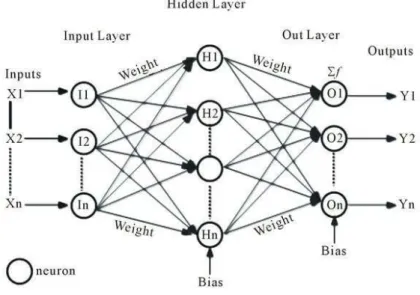
Usually, neural networks consist of more than one neuron. Figure 2 visu-alizes a so-called feed forward multilayer network. Each layer’s neurons are connected to all neurons of the next layer. The input layer takes the initial inputs and transmits them to forward through one ore multiple so-called hidden layers, which are not observable from the outside. Finally, the signals reach the output layer, whose amount of neurons determines the size of the output space. Each output neuron produces a score Yi which can be used to

take decisions or predictions.

In supervised training, the correct results for training data are known, which allows to define a loss function that measures the greatness of the

(15)

Figure 2: Multilayer neural network with hidden layer in between (Fumo (2018)).

error in the prediction. This loss value can be used to train a neural network’s weight parameters by computing the gradients backwards and updating them in order to minimize the error for further future predictions. This process is called backpropagation and allows the neural network to automatically learn from its mistakes and to improve itself.

For example, a common usage of a neural network is the task of image classification. Assuming that the inputsairepresent significant features of the

original image, each of the final outputs Y stand for a possible class that the image may belong to. A high score indicates a high probability that the image belongs to that class. Besides image recognition, neural networks became famous for solving problems in many other areas like speech or language processing. Regarding the task of question answering, neural networks can be built in such a way they take the words of question and answer sentences as input features. Based on this, they can produce a prediction, saying which of the candidate possibilities is most likely the correct one to that question.

(16)

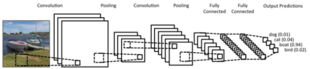
Figure 3: Convolutional Neural Network with multiple convolutional filter and pooling layers (Fumo (2018)).

3.2.1 Convolutional Neural Networks

Convolutional neural networks (CNNs) are a special kind of neural networks:

In fully connected layers as described above, for an input feature like a pixel in the task of image processing, its location in the image is not considered, as each input feature is connected to all neurons in the first hidden layer in the same way. The idea of convolutional filters is to take only small regional windows of an image at once that are connected to one hidden neuron. The convolutional filter then moves over the whole image and produces one output for every position while applying the same weights and bias for every step. This way, a filter (sometimes also called kernel) produces a feature map for the whole image that captures regional properties and patterns. Usually, many different filters are applied that aim to detect different features of the input. In the next step, the most meaningful information of the produced feature maps is often extracted using so-called pooling layers. For instance, a common pooling technique named max pooling simply takes the maximum of output values in the previous layer in a certain region. This helps the network to concentrate on the most significant features found during convolution and to reduce the number of needed weight parameters for following layers (Kim (2014)). Figure 3 shows this process with several subsequent convolution and pooling steps before a final classification is performed with some fully connected layers.

(17)

In the same way as for image recognition, convolutional networks can be built for the purpose of textual understanding (Kim (2014)). One sentence consists of several words, of which each again can be represented as a multidi-mensional vector (see Section 4.1.2). This results in a sentence matrix where convolutional filters are able to extract features considering word order and regional context.

3.2.2 Attention Mechanisms

The idea of so-calledattention in the context of deep learning is reminiscent of the human ability to focus on particular objects or spots in his view. These objects get sharper, while the rest of the image stays blurred. In the same way, a neural network can concentrate on information considered relevant for a specific task (Tian (2018)). For natural language processing, particu-larly for question answering, this can be achieved, for example, by focusing on meaningful words in the answer sentence that appear somehow related to those in the question. Hence, such words can be assigned with stronger weights. The attention weights can be determined, for instance, by comput-ing dot products between all word vectors from the question and all those from the answer sentence that should be matched. In contrast to the so-called hard attention techniques, a text comprehension model using this soft attention stays fully differentiable and still allows the computation of the backpropagation.

4 Resources

4.1 Tools and Frameworks

In this section, some additional libraries will be described in detail that were used for network construction and during the experiments.

(18)

4.1.1 TensorFlow

From a technical point of view and concerning neural network implementa-tion, besides well-tried solutions like Theano or Torch, the relatively new

Ten-sorFlow framework is currently enjoying great popularity. The open source

machine learning tool was developed by Google, or more precisely the Google Brain Team. It was first released in 2015 and represents the successor of the previous tool DistBelief. Compared to this, it scores mainly on greater flex-ibility and portability (Simon (2018)). TensorFlow models can be executed in different environments like CPU or GPU and even on mobile or embed-ded devices without having to port the code. Furthermore, the tool is highly scalable and supports parallel executions. The additional tool TensorBoard simplifies the display of aggregated execution summaries.

The implementation of new neural models is achieved by constructing a computational graph. The nodes of this graph are executable numerical op-erations, while the edges represent the tensors. Tensors are data arrays with multiple dimensions that “flow” between the different nodes. New models can be easily built and extended with the existing building blocks taken from the TensorFlow toolkit in a high level programming language like Python, C++, Go or Java.

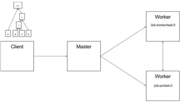
Figure 4 illustrates the core architecture of the framework. In the client layer, the computational graph is created and prepared for execution. There are many libraries with a high level of abstraction that help to facilitate this process. The computed graph is then initiated within a TensorFlow session and passed to the (distributed) master. The master is responsible for par-titioning and distributing the execution of subsets of the graph operations to one or several workers, which may reside on different devices and/or in additional processes. Figure 5 shows this interaction between the different TensorFlow components. In this example, /job:ps/task:0 is the parameter server and responsible for managing and updating the model’s parameters, which may be triggered by operations on the other worker. Note that instead

(19)

Figure 4: Core architecture of the TensorFlow framework (The TensorFlow Team (2018)).

Figure 5: Communication between TensorFlow components (The TensorFlow Team (2018)).

(20)

of using this distributed behavior, of course also all computation can be done by a single process. However, the real strength of TensorFlow shows in its automatic parallel optimization techniques when applied to a distributed system. The kernel operations, which represent single core graph operations and of which more than 200 are existing at the moment, are mostly imple-mented in C++. They also support efficient execution also on GPUs through a binding to NVIDIA’s CUDA and cuDNN libraries. Additionally, they can be expanded by the community if a new operation is required. For these rea-sons, this flexible, highly scalable tool with growing community support was considered a good choice for the purposes of this thesis.

4.1.2 GloVe

GloVe stands for an algorithm that is able to train global word

representa-tions in the shape of high dimensional vectors (Pennington et al. (2014)). During training on large corpora it catches some statistics of word occur-rences and the frequency of their appearances in a context together with other words. This information is reflected in the final trained vector rep-resentation of a word and allows to execute tasks of similarity or analogy, for example, to find the most similar neighbor word. This is very useful for purposes of text comprehension, since a neural network model is able to rec-ognize related words by considering the relatedness of their mathematical representations in the vector space. For this thesis, an existing GloVe model was taken that was pre-trained on common web crawl data with 840 billion tokens, a vocabulary size of 2.2 million words and vector dimensions of 3002

.

4.2 Datasets

To measure the performance of the created neural network, it was trained and tested on three benchmark data sets, namely MovieQA, WikiQA and

2

(21)

Figure 6: Data statistics for the three data sets. Q = question, C = candidate answer, P = plot (Wang and Jiang (2016)).

InsuranceQA. The first one contains question-answer sets demanding the comprehension of movie contents and actions. The second one is a collec-tion of query logs and wiki pages from Wikipedia. Finally, the contents of

InsuranceQA are all about the insurance domain, the questions come from

customers and ask for information about different kinds of insurances. Al-though all data sets contain questions and a set of multiple choice candidate answers, each of them comes with a slightly different task and provides quite different statistics, as Figure 6 reveals. The individual data sets and their properties will now be explained in detail.

4.2.1 MovieQA

The data set consists of a collection of 14,944 question and answer sets taken from 408 movies and collected by human annotators, while the questions may vary from simple ’who’ or ’when’ to more complex ’why’ or ’how’ question types. Each question comes with five possible candidate answers of which only one is the correct answer to the question. Therefore, the task for a system is here to predict that one correct answer.

As an additional support for answering the questions, the data set con-tains several different sources that provide further information about the movie contents: Plot synopses are texts written by fans who have watched

(22)

the movie and mostly describe the actions happening in the story. Videos are provided as clips together with their subtitles and are referenced via timestamps. Besides,Described Video Service (DVS)files are available, which contain narration texts of movies for visually impaired people and thus are including also descriptions of visual details of the movie. Finally, script files written by screenwriters are included which usually contain both, information about a scene, and the intended dialogs of the actors in the final movie.

All of these data sources are aligned to the corresponding movie and referenced in the question sets as JSON files as shown in the example of Listings 1 and 2. The first one is an excerpt of the movie database containing one single entry, namely The Lord the Rings: The Return of the King. Here all available additional sources of information are linked together with the ID of the movie. This allows one question-answer sample like that one shown in the second listing to reference textual or visual support files like the movie’s plot, script or subtitles. Also the index of the correct answer and the plot sentence(s) containing a hint to the correct answer are given here.

Thus, all aligned data can be accessed as an additional source of informa-tion by any quesinforma-tion-answer problem to be solved. Another sample quesinforma-tion is given in Table 1 together with its five candidate answers and an excerpt of the corresponding movie plot which contains the necessary information to answer the question. For this work, only plots are used as they provided the most promising results in all previous works3

. Note that the accuracies for the test set can only be computed online on the authors’ server because the correct labels are not included in the download files of the data set. The data set includes simple data loader classes that allow to load and access all data from within python.

3

(23)

{

"genre": "Adventure, Fantasy", "text": { "plot": "story/plot/tt0167260.wiki", "subtitle": "story/subtt/tt0167260.srt", "dvs": null, "script": "story/script/tt0167260.script" }, "imdb_key": "tt0167260",

"name": "The Lord of the Rings: The Return of the King", "year": "2003"

}

Listing 1: Example from MovieQA’s movies JSON file

{

"qid": "val:1683",

"question": "How is the Ring finally destroyed?", "answers": [

"Sauron gets bored of it and throws it into the volcano",

"Gollum breaks it",

"Sam throws it into the fire",

"Frodo burns it",

"It is consumed by the fire when Gollum falls with it in his hand"

], "imdb_key": "tt0167260", "correct_index": 4, "plot_alignment": [ 31 ], "video_clips": [ "tt0167260.sf-303781.ef- 307282.video.mp4" ] }

(24)

Question Where does Sam marry Rosie?

Plot

... Aragorn is crowned King of Gondor and taking Arwen as his queen before all present at his coronation bowing before Frodo and the other Hobbits. The Hobbits return to

the Shire where Sam marries Rosie Cotton. ...

Candidate answers 0) Grey Havens. 1) Gondor. 2) The Shire.

3) Erebor. 4) Mordor.

Table 1: MovieQAexample question (Wang and Jiang (2016)).

4.2.2 WikiQA

The WikiQAdata set was originally collected by Microsoft’s research group

(Yang et al. (2015)). It consists of 3,047 questions extracted from collected query logs taken from Microsoft’s search engine bing. Each of the selected questions forwarded the user, who had entered the query, to a Wikipedia page about this topic. As each of these pages contains a paragraph that summarizes the most important contents, each sentence of this paragraph was taken as a candidate answer for this data set. For this reason, the number of possible answers variates for WikiQA. A typical WikiQA question-answer set originally looks like this:

Question: Who wrote second Corinthians?

Second Epistle to the Corinthians The Second Epistle to the Corinthi-ans, often referred to as Second Corinthians (and written as 2 Corinthians), is the eighth book of the New Testament of the Bible. Paul the Apostle and “Timothy our brother” wrote this epistle to “the church of God which is at Corinth, with all the saints which are in all Achaia”.

Here, the question is listed together with its corresponding summary para-graph of Wikipedia, where each sentence will result in an answer possibility.

(25)

Each candidate was annotated by several human workers with YES, if the sentence provided a correct answer to the corresponding question, or

with NO, if it did not. Therefore, on the one hand, there are questions with

multiple correct answers where several sentences of the paragraph provided a valid answer. On the other hand, the data set contains a lot of questions (about two thirds) that do not come with any correct answer, in case the summary paragraph did not provide any. As these questions are of special interest, for instance, in the field of answer triggering, but are not suitable to answer selection tasks, the questions with no correct answers have been excluded in this approach as done by Wang and Jiang (2016). This results in a relatively small data set with only 873 samples for training, 126 for validation and 243 for the test set, as Figure 6 shows.

In contrast to both of the other data sets, the task ofWikiQAis not only to find one correct answer since there may exist multiple ones, but also to rank the candidate answers according to their likelihood of answering the question. For this reason, the success of a model for WikiQAis not measured in terms of accuracy, but rather with metrics of mean average precision (MAP) and mean reciprocal rank (MRR).

4.2.3 InsuranceQA

The InsuranceQA corpus consists of question and answer sets concerning

the insurance domain collected from the website Insurance Library4

, where experts can be asked all kinds of questions about insurances. With a total amount of 24,981 answers, this data set provides the biggest answer pool in this work. Each question comes with a so-called ground truth set, which contains one or several correct answers to the question. In this case, the corresponding goal is to determine the best candidate answer for a given question out of a big pool that contains the ground truth set and is filled up with wrong answers. For the InsuranceQA task, a question is considered as

4

(26)

Question can i have auto insurance without a car

Ground-truth answer

yes, it be possible have auto insurance without own a vehicle. you will purchase what be call a name ...

Other (wrong) candidate answer

insurance not be a tax or merely a legal obligation because auto insurance follow a car...

Table 2: InsuranceQA example question (Wang and Jiang (2016)). answered correctly, if the candidate answer predicted by a model lies within the ground truth set.

Table 2 shows an example question together with its ground truth and another incorrect candidate answer. As the sentences reveal, all of the word sequences were parsed with the Stanford Tokenizer5

before. Also, in contrast

to MovieQA and WikiQA, the text of this corpus has already been

lemma-tized. For the validation and test set, the answer pools are fixed with a size of 500 questions in total. For training, the pool’s size and wrong candidate answers can be chosen freely for a question from the total pool of answers. The approach for building the answer pool used in this work is described in Section 6.1.1.

5 Network Design and Implementation

5.1 Considerations

When starting this thesis, one of the most promising approaches for sequence matching problems and, thus, also for question answering, was provided with the CNN matching network by Wang and Jiang (2016). The great advantage

5

(27)

of this contribution lies in its generality. As the authors demonstrated, their network structure can be applied to question-answer data sets that come from different domains and have slightly different tasks without the need for greater changes. Furthermore, they optimized their model regarding different comparison functions between sequences of words. In these experiments they achieved quite impressive results (see Section 6.2.1 for all tested data sets compared to the original proposed baselines, which are MovieQA (Tapaswi et al. (2015)),InsuranceQA(Feng et al. (2015)),WikiQA(Yang et al. (2015)) and SNLI (Bowman et al. (2015)). In addition, parts of the source code were made public6

, which facilitates reimplementation and reproduction of results. For these reasons and in order to receive a flexible text comprehension system that might be extendend for future tasks even after creation, the approach of Wang and Jiang (2016) was reimplemented with the framework TensorFlow and serves as a baseline for this work and for all further experiments. All data sets except forSNLI are supported by this reimplementation, since this huge corpus would have required a lot of additional resources and time for training. Also, the corpus does not contain question-answer sets, but rather statement sentences for the task of textual entailment.

Although generally following this CNN matching network approach, some details have been modified in the TensorFlow reimplementation. Therefore, in the following sections, design and implementation of the baseline model will be described in detail.

5.2 Network Design

As mentioned before, the general idea of this approach is to build a so-called compare-aggregate system. Hence, the basic thought is to match two text sequences by first comparing them word by word and then aggregate the comparison result with a convolutional layer for the final prediction. For the aim of question answering, the model’s task is to decide whether a

6

(28)

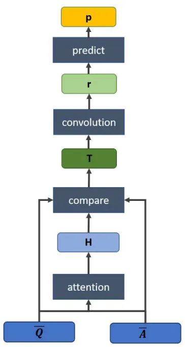
Figure 7: Model layers for WikiQAandInsuranceQAfor a prepared question

(29)

Figure 8: Preprocessing layer with question lengthQ, candidate answer length

A, GloVe word embedding size d and layer output sizel.

potential candidate answer text sequence is probably a correct answer to a given question sequence or not.

Figure 7 shows the layer flow of the model in its final implementation, which will be explained in detail subsequently. For the network description it is assumed that for one input sample, in each step there exists a question

Q and a candidate answerA, that needs to be matched against the question with the help of the neural network. This process is explained for one question and one candidate answer, as each of them is compared to the question separately. Only in the final layer the scores of all candidates come together for making a prediction.

5.2.1 Preprocessing Layer

After prepocessing the data as explained later in Section 5.3.2, Qand A are available as sentence embeddings with Q ∈_RQ×d

and A ∈ _RA×d

, where Q and Aare the length of question resp. answer and d is the dimension of the word vectors.

Both Q and A now run through an additional preparing layer shown in Figure 8, which projects the high dimensional word embeddings to a lower output size l in order to reduce the number of needed parameters for subse-quent layers. This step is done as follows:

X =σ Wi_X₊_bi

(30)

Here ⊙ indicates element-wise multiplication. Wi, Wu ∈ _Rl×d

and bi,

bu ∈ _Rl are trainable parameters that produce new embeddings of size l.

These weights and biases are reused for both preparing question and answer sequences. Thus, applying this layer finally results in the new embeddings

Q ∈ _RQ×l

and A ∈ _RA×l

. As proposed by Wang and Jiang (2016), some dropout is performed on the initial word embeddings before feeding them into the projection layer, too. Especially for WikiQA this becomes important in order to prevent overfitting since the training data set is very small. Details are discussed in Section 6.1.1

5.2.2 Attention Layer

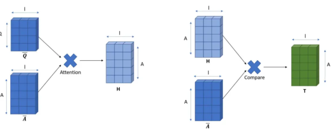
The second layer aims to create an attention-weighted version of the question regarding a specific candidate answer. This means that those words in the question that are most related to individual words in the answer sequence are emphasized in a way that the model will pay more attention to them. Therefore, the attention weight matrix G∈_RQ×A

is constructed first:

G=sof tmaxQTA

Note that in contrast to Wang and Jiang (2016), the learnable parameters have been left out of the attention layer in this work because they seemed to provide no help in this approach but rather decreased evaluation accura-cies during the experiments. The attention weight matrix is then multiplied with the question for generating an attention-weighted version of the answer, labeled as H∈_Rl×A

:

H=QG

In detail, each weighted vectorhj inHrepresents that part of the question

which best fits to the corresponding word vectoraj of the prepared candidate

(31)

Figure 9: Attention and comparison layer with question-weighted answer vec-tors H.

5.2.3 Comparison Layer

The next step is done by a comparison layer that matches each hj inHwith

its counterpart aj, which is also visualized as part of Figure 9. While Wang

and Jiang (2016) experimented with many different comparison functions, here, only the two most convincing functions are chosen that provided best results in their work. The first one, labeled as MULT, consists of a simple multiplication of the vectors:

MULT:tj =aj ⊙hj

This function proved to be best for small data sets like WikiQA and is, thus, used in the present work for this task, too. For the other tasks,MovieQA

and InsuranceQA, the following SUBMULT comparison function is used:

SUBMULT:tj =ReLU(W " (aj −hj)⊙(aj −hj) aj ⊙hj # +b) Here, W∈_Rl×2l

and b ∈_Rl are trainable parameters again. The

(32)

Figure 10: CNN and predcition layer with nl = number of different kernel heights × kernel number each. K = number of candidate answers.

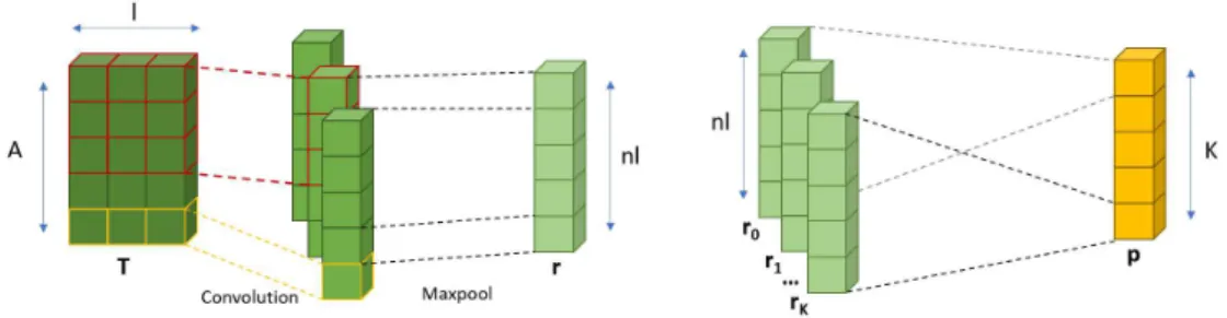
5.2.4 Aggregation Layer

In the following step, the vectors tj are aggregated using a one layer CNN,

as proposed by Kim (2014):

r=CN N([t1, ...,t_A])

CNN internally consists of a convolutional layer with kernels W ∈ _Rk×l×l

, wherekis the kernel height andl again determines kernel width and number of kernels. As shown in Figure 10, each convolutional layer is followed by a max pooling layer, which reduces the feature maps to r ∈ _Rnl, where n

stands for the number of different kernel windows used. Finally, the resulting

rrepresents the features of one candidate answer, which can be used together with the features of the other candidates in a prediction layer.

5.2.5 Prediction Layer

The final prediction layer, which is visualized on the right side of Figure 10, uses the precomputed features R = [r1, ...,rK] of K candidate answers to

make a prediction:

p=sof tmax(wT _tanh(_Ws_R₊_bs

) +b)

with Ws _∈ Rnl×l

, bs ∈ _Rl, w ∈ _Rl and bs ∈ _R. The resulting p ∈ _RK

(33)

which answer is considered most likely to be correct. Note that the prediction scores for all candidate answers are computed separately for everyrK before

the softmax function, but in contrast to classical classification tasks the same weights and bias are shared for all final dense layers. The softmax function is used here only for smoothing the results in order to receive a valid probability distribution.

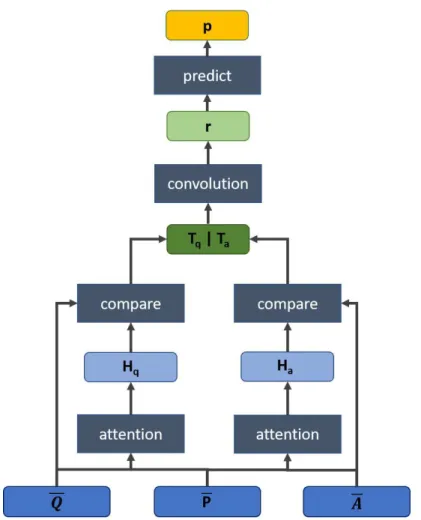
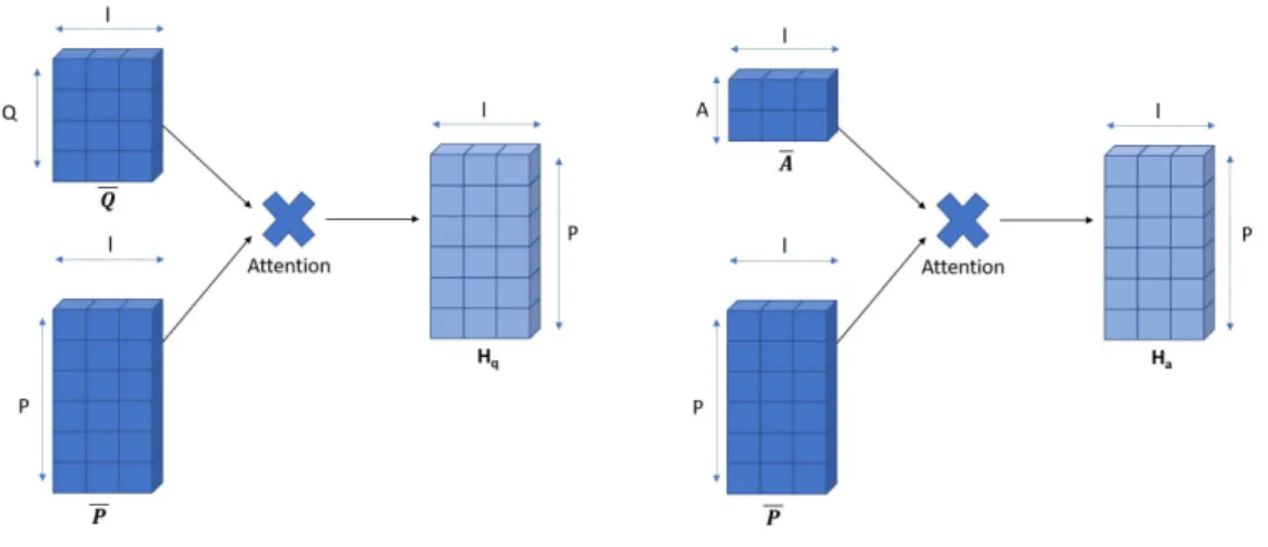
5.2.6 Task-Specific Adaptations

For theMovieQAdataset, the model as it has been described so far has to be adapted slightly. An overview about the changes are given by Figure 11: Since there are three sequences to be matched, namely question, candidate answer and plot text, the question is compared to the whole plot sequence first by sending both through the attention and comparison layers shown in Figures 12 and 13. In accordance, every candidate answer is compared to the plot again by sending both through the same layers with identical weights as for processing the question. The results of both question and answer comparisons with the plot are then merged together before the aggregation step in the convolutional layer of Figure 14 as follows:

tk,j = " tqj ta k,j #

This way, the convolutional filters regard features of question as well as answer weighted plot and extract significant features of both at once. After the convolution, the prediction is computed in the same way as described for the other data sets.

(34)

Figure 11: Model layers for MovieQA. The additional plot resource P is matched with both Q and A.

(35)

Figure 12: Attention layer forMovieQAtask. Here the whole plot is weighted with both question and candidate answer.

Figure 13: Comparison layer for MovieQA task. Question and answer are compared to their weighted plot version.

(36)

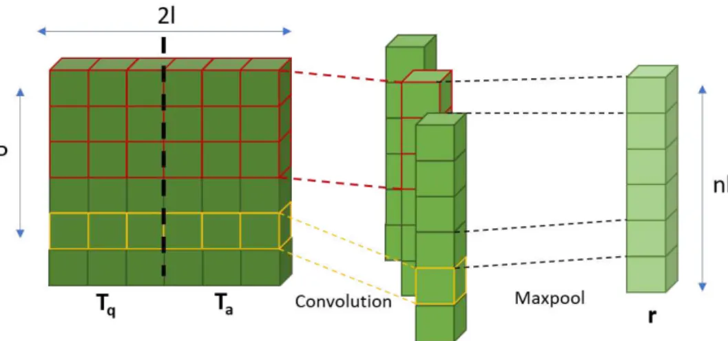
Figure 14: Convolutional layer for the MovieQA task. Question and answer weighted plots Tq and Ta are concatenated right before the convolution.

5.3 Implementation Details

5.3.1 Environment Setup

The implementation of the baseline model as well as all experiments were run using a GPU compatible version of TensorFlow (v. 1.5) together with a python 3.6 environment. This programming language provides the most supported frontend with the currently biggest community where many high level interfaces are provided for creating neural networks. All data sets were downloaded, extracted and prepared for their usage within the TensorFlow framework. Note that this work uses version V1 of the InsuranceQA data set for being comparable to the work of Wang and Jiang (2016), although version V2 is already available7

.

5.3.2 Data Preprocessing

As introduced in Section 4.1.2, the inputs of the system are built upon pre-trained word embeddings taken from a GloVe model with vector dimensions

7

(37)

of d=300. For the simple baseline model, the embeddings are not updated during training. In a first step, all sentences in every data set are converted into a matrix of shape n×d, where n is the number of words in a sentence and d the dimension of the word embeddings. If there is no representation available for a word, the vector is initialized with a small random uniform vector with values between -1.3 and 1.3 as most embedding values lie in this range. Every used word representation is saved in a vocabulary dictionary and is referenced by its key.

For every sentence the word keys are stored under their context (question, answer or plot), usually in TensorFlow’s TFRecord format, which is based on Google’s protocol buffer format. This way, the whole data set is being included into the computational graph and can be loaded, batched and shuf-feled by TensorFlow models easily. Also, storing of the labels varies among the different tasks: ForMovieQA, where there is only one correct answer to a question at any time, the label entry in the record file is written as a simple one-hot vector. For WikiQA, on the other hand, there may be several cor-rect answers among the candidates. In this case, every corcor-rect label is first assigned with 1 and then divided by the total amount of correct answers for this question. This way, the label vectors sum up to 1 and can be used as a well distributed input for a loss computation with softmax and cross-entropy during training for optimizing the model.

For InsuranceQA, as mentioned above, only the correct answers for a

question are given for the training set by default. So during preprocessing only each correct answer is stored together with its question as one single sample that gets filled up with wrong answers later. This way they can be exchanged easily by other random candidates from the whole answer space in every new epoch.

(38)

6 Experiments

6.1 Experimental Setup

For the tasks of evaluating and improving the baseline built in Section 5, sev-eral experiments were performed on the existing model. To measure the suc-cess of the created neural networks, accuracy of correctly answered questions has been used during all experiments, except for WikiQA, which requires ranking of answers and, thus, is evaluated by computing mean average pre-cision (MAP) and mean reciprocal rank (MRR).

First of all, an attempt was made to get better evaluation accuracies by fine tuning the hyperparameters of the network. In a second experiment, the existing pre-trained GloVe word embeddings were replaced by updateable embeddings. Besides, for MovieQA the model was extended with a second stage of attention and convolution on sentence level for the plot text. Finally, for inferring the model’s internal learning state and limits, it was evaluated using adversarial samples.

6.1.1 Hyperparameter Setting and Tuning

The performance of a network strongly depends on its setting of parameters. Therefore, in order to improve the results which have been achieved with the baseline, the initial network’s parameters have been tuned in search for an optimized configuration. For finding good choices for the model’s hyperpa-rameters, a greedy approach was chosen which tried to variate one parameter after another and always took that configuration providing the best results, i.e. achieving the highest validation accuracies or precisions and the lowest total loss, into the next steps. For each parameter’s tuning, at least five dif-ferent models were trained on every tested setting for ensuring significance of the results.

(39)

Karpathy (2018), different TensorFlow weight initializer implementations were tested. The following initializer functions were tried out:

• tf.contrib.layers.xavier initializer8 with uniform distribution • tf.random uniform initializer9 with values between -0.1 and 0.1 • tf.variance scaling initializer10

• tf.truncated normal initializer11

• tf.random normal initializer12 with a mean of 0 and a standard

deviation of 0.1

Whilerandom normal andrandom uniform initializerscompute the weights without regarding the input or output sizes of layers, this is indeed done by

the xavier and variance initializers with the aim to keep the gradients in the

same scale through all layers. The truncated normal initializer is similar to the random normal initializer, but here outliers that deviate to far from the mean are thrown away and newly computed. All of the described initializers were tested with the standard settings listed here in order to observe which one contributes to the best score with the given model.

During the experiments, also three different optimizers for updating the weights were tested out: A standard stochastic gradient optimizer (SGD), the Adam optimizer (Kingma and Ba (2014)), and the Adamax optimizer, a variation of Adam which was also used by Wang and Jiang (2016).

Furthermore, for the optimization of the model, two different loss func-tions were evaluated: A standard cross entropy loss function and a variant of

8

https://www.tensorflow.org/api docs/python/tf/contrib/layers/ xavier initializer.

9

https://www.tensorflow.org/api docs/python/tf/random uniform initializer.

10

https://www.tensorflow.org/api docs/python/tf/variance scaling initializer.

11

https://www.tensorflow.org/api docs/python/tf/truncated normal initializer.

12

(40)

the hinge loss, in which the margin between the scores of correct and wrong answers to a question is tried to be maximized with:

Lhinge=max(0,(smaxW rong−scorrect+m))

WheresmaxW rongis the biggest score among the wrong candidate answers,

scorrectis the score of the correct answer andm = 1 is the margin between the

scores that is tried to be achieved. If there are multiple correct answers (as it is the case for the WikiQA dataset), the loss is computed for each correct answer and the highest value is chosen for the optimizing step. Using this formula, the loss is 0 if the margin between the two scores is high enough.

For the single dropout on the initial word embeddings, different dropout rates of 0.1, 0.2, 0.4, 0.6 and 0.8 were tried out. If necessary, the experiment was repeated with more fine grained values that lay between the initial ones. While fine tuning the learning rates, values of 0.01, 0.001 and 0.0001 were tried out first. Afterward, the best configuration was taken and fine-tuned using smaller variations.

The batch size was set to 30 for all runs and not tuned during experiments. Also, L2 regularization has been added to the loss function to penalize outliers among the weight updates. The beta scale of the regularization function was tested with values of 0.01, 0.001 and 0.0001. Within the convolutional layer, fixed filters with different kernel heights were used: [1,3,5] forMovieQA and [1,2,3,4,5] for both WikiQAand InsuranceQA. The number of kernels is set to 150 for each individual kernel and their resulting feature maps are concatenated after max pooling. The number of output units l has been set to 150 for all other (dense) layers.

Note that for InsuranceQA, the training data set is not fixed and only the true answers for a question are given. The pool of negative answers still had to be built by taking random wrong answers from the total answer pool. These negative answers are resampled every epoch. Although the results of Wang and Jiang (2016) were claimed to be achieved with a training pool

(41)

size of 50 candidate answers, it was also tried out with a size of 100 during training, hoping to achieve better results this way on the big test sets with 500 candidate answers per question.

6.1.2 Updated Embeddings

Since in most of the related works the word embeddings were not updated during training of the model, this attempt was made in the scope of this work in two ways: First, pre-trained GloVe vectors were used as described so far and updated during training in every batch step. In a second experiment, all word vectors were initialized as random uniform distributed vectors with values from -1.3 to 1.3 (in which areas most of the glove vector values lie) and updated every batch step, too. Both experiments were performed for the

WikiQA task first, as this small data set needs the least training time.

6.1.3 Sentence Attention

As described before, MovieQA uses an additional textual source, the movie plot, which consists, compared to question and answer phrases, of a rather large text. For this reason, an attempt was made to include an additional level of attention to the model, namely sentence level attention, as also proposed by Liu et al. (2017). Because their model variates from the baseline which is followed in the present work, this sentence attention concept could not be transferred completely the way it was described there. Nonetheless, the core idea to match each sentence of the plot with question and candidate answer separately instead of taking the whole plot at once was adopted for a corresponding extension of the baseline model.

Figure 17 illustrates the first stage of this process: For every plot sen-tence Pi with length ofps words, the feature maps are computed exactly the

same way as before and are fed into the convolutional layer shown in Fig-ure 18, which creates a question and answer weighted featFig-ure set for every

(42)

Figure 15: Stage one of sentence attention model produces sentence features

(43)

Figure 16: Stage two of sentence attention model produces final features rs

(44)

Figure 17: Preparation step for MovieQAwith sentence attention. Each sen-tence of the plot is processed separately and matched to question and can-didate answer instead of taking the whole plot at once.

plot sentence. The initial prepared question and answer features are now sent through the same convolutional layer (i.e. with the same weights). Therefore, both are duplicated and concatenated for fitting to the convolutional filters used for the creation of rpi.

The output results of this first stage’s layers are feature sentence repre-sentations for question, answer and a plot sentence. In the following, these outputs of the first stage are used as inputs for the second stage of sentence level processing, of which Figure 16 gives an overview. In the beginning, the plot sentence features are all concatenated again, as Figure 19 indicates. Then, the whole plot runs through another attention step where its sentence features are weighted with the sentence features of question and candidate answer again (Note that both are considered to consist of exactly one sen-tence). What follows is another comparison step for both weighted plots. For this second comparison layer, new weights are used, but they are shared for both question and answer weighted plot comparison again.

Finally, the resulting question and answer feature maps Tqs and Tas are

concatenated again and fed into another convolutional layer with new weights, which is shown in Figure 20. The process described so far reduces the features

(45)

Figure 18: Stage one output sentence representation of plot sentence, question and answer with one shared convolutional layer.

(46)

Figure 19: Second attention step on sentence level of stage two for question

rq and answer ra with concatenated plot sentences [rp0, r_p1, ..., r_pi].

Figure 20: Second convolutional layer for final feature representation rs of

(47)

of all plot sentences to one feature vector of length nlper candidate answer. These vectors are then, again, used for the prediction layer in the same way as done before.

6.1.4 Adversarial Examples

The idea of adversarial examples is to fool or confuse a model by manipulating the given information as done by Jia and Liang (2017) for the field of text comprehension. This approach aims to show how deep the true understanding of the network really is. In this work, during the experiments the plot for the

MovieQAsentence attention model was modified in that part of the text with

the strongest textual attention, which is the first contribution of this kind to the best of own knowledge. After changing the plot, the model was evaluated to see whether it concentrated on the right section of the text and if it is still able to answer the question correctly when the context changes.

Therefore, in a first step, some words of the plot were changed within that sentence getting the most attention by the model. For these experiments, a single model was chosen and modified twofold: In one approach, 1 to k random words were exchanged by other random word representations taken from the vocabulary. In a second approach, the 1 tok most attention weighted words in that sentence were exchanged. By this setting, the effect of word attention is observed and compared to the strategy of randomly taking out words.

Additionally, for evaluating how well the model is able to understand and answer the question correctly compared to a human being, a small evaluation set of 20 randomly chosen samples was taken from the validation set and observed manually. A question was considered as answerable correctly by a human, if the right answer could be recognized among all candidates only with the help of the (remaining modified) plot text. Table 3 contains an example of the original and modified plot for a question. As one can see, in the manipulated plot the right answer name is still appearing in the sentence,

(48)

Question What is William’s mother’s name?

Original plot His mother Elaine wants him to become a lawyer.

Modified plot (k=3) Autua argo Elaine wants him to firing a lawyer.

Candidate answers 0) Shunn. 1) Ann. 2) Anita.

3) Elaine. 4) San.

Table 3:MovieQA adversarial example question with modified plot sentence based on word attention and with k=3 exchanged words.

but the context ofmother has gone, so the model will probably fail to answer this question and also a human could not answer it anymore with the modified plot sentence.

Finally, there was an attempt of improving the overall model performance by training it with a portion of adversarial examples. This training happened with the hope to stabilize the model and to achieve better results when it is tested on modified plots. So after training, it was tested in the same way as in the beginning in order to compare how the results changed. For a better understanding of the attention layer’s effects within the neural network mod-els, especially during the adversarial experiments, an visualization plotting function was added that illustrates the attention weighted word features as a heatmap at the state of the convolutional layer (see Sections 6.2.4 and 6.2.5).

6.1.5 Ensemble Model

For every data set an additional ensemble model was built that consists of a combination of nine fine-tuned single models for MovieQA and five for

WikiQA and InsuranceQA. The ensemble models choose the correct

candi-date answer(s) by majority vote and were created with the aim to provide a greater stability of predictions. For MovieQA, this model also was used to create a file with predicted labels for the test set, which was submitted to the server provided by the authors for the final evaluation of the system’s performance on this task.

(49)

MovieQA WikiQA InsuranceQA

Val. Test Val. Test Val. Test

Baseline 73.23 - 72.50 - 63.70

-Tuned Model 75.60 - 76.39 73.45 73.60 73.27

Updated Embeddings - - 70.41 - -

-Sentence Attention 80.69 - - - -

-Ensemble Model 82.89 82.73 76.29 75.51 73.20 74.10

Table 4: Overview experimental results.

6.2 Results and Discussion

This section presents all experimental results for the settings described so far. First, an result overview over all experiments performed is given and the achieved scores are compared to those of related works. Afterwards, all individual experiments and their outcomes will be discussed in detail.

6.2.1 Overview

Table 4 shows the evolution of the accuracy scores from the initial Tensor-Flow baseline to the final models. The experiments have been performed in the order in which they are listed above and each one was built on its pre-decessor’s best result. As one can see, the building of ensemble models has a notable effect on the performance, since it increases stability of the answer decisions, except for WikiQA, where one single model performed best (re-member that the results of this corpus are given by terms of mean average precision instead of accuracy). In contrast, the updated embeddings made the systems perform even worse than the baseline with no updated embed-dings. On the other hand, the introduction of the sentence level attention lead to a great improvement of more than 5% for MovieQA. The adversarial experiment’s final result is left out here because its testing context differs from the other results and cannot be displayed as a single value as explained

(50)

MovieQA WikiQA InsuranceQA

Val. Test MAP MRR Val. Test

Yang et al. (2015) - - 65.20 65.20 -

-Feng et al. (2015) - - - - 65.4 65.3

Tan et al. (2015) - - - - 68.4 68.1

Wang and Jiang (2016) 72.1 72.90 74.33 75.45 77.00 75.60

Liu et al. (2017) 79.00 79.99 - - -

-Dzendzik et al. (2017) - 80.02 - - -

-Min et al. (2017) - - 83.20 84.58 -

-Own Work 82.89 82.73 76.39 76.41 73.60 74.10 Table 5: Related work overview

in Section 6.2.5. The best adversarial accuracies on the unchanged evaluation set lie in the same range as the model with sentence attention.

As Table 5 shows, the TensorFlow reimplementation of the approach of Wang and Jiang (2016) achieves competitive results for the WikiQA data set compared to the original work, but does not reach the state-of-the-art approach by Min et al. (2017). In their work, the model’s parameters (in-cluding word embeddings) were pre-trained with data from SQuAD. This data set also comes from the domain of Wikipedia, but with 100k training samples the corpus is about 100 times bigger than WikiQA. Thus, training the embeddings and model weights on this huge corpus and only fine-tuning

onWikiQAresulted in far better results than they could be achieved by this

work. Since training on such a large corpus would have required a lot of ad-ditional efforts, this experiment proved to be impracticable for the scope of this work and remains as a future work.

For MovieQA, the results could be improved quite a lot by combining

the original compare-aggregate approach with the sentence level attention, which was inspired by Liu et al. (2017), but realized slightly different. The ensemble model, which was created out of these single models, outperforms

(51)

all current approaches of knowledge for MovieQA13

, including the work of Dzendzik et al. (2017), who held the top of the leaderboard for a longer time with their approach using logistic regression over sentence similarities. This improvement in comparison to all previous works goes back to the additional implementation of the second stage with attention on sentence level for the biggest part and may also be due to the fact that random vectors for unknown word representations are used here instead of initializing them with zero vectors as in the original work by Wang and Jiang (2016).

ForInsuranceQA, although also following exactly the same approach and

implementation, in contrast to WikiQA this implementation still lies some percents behind the results provided by Wang and Jiang (2016), which is kind of surprising. Although not having published the source code for this data set, in a discussion on their GitHub page14

the authors claim that the model structure for InsuranceQA is exactly the same as for WikiQA. The only difference mentioned there is the construction of the answer pool, which besides the one correct answer is filled up with 49 wrong candidates that are reassigned each epoch. So the most obvious reason why the TensorFlow reimplementation performs worse is that the exact process of how the answer pool is preprocessed and created might differ from the original work in some significant details. While working on this thesis, theMovieQAdata set turned out to be of greater interest because of its additional textual resources like the plot. Therefore, no further investigations for improvingInsuranceQAwere made, but instead the MovieQA was focused more in the subsequent work.

So all in all, the created comprehension system could outperform all re-cent works onMovieQA, but could not beat the state-of-the arts for the other data sets. The reasons for this gap go back to MovieQA’s adapted sentence attention model, which in combination with the general compare-aggregate structure provides a novel mechanism to find and focus the correct sentence with the hint to answer a question with a high probability. For WikiQA and

13

Seehttp://movieqa.cs.toronto.edu/leaderboard/.

14

(52)

WikiQA MovieQA InsuranceQA Initializer xavier xavier xavier

Optimizer Adam Adam Adam

Loss function entropy entropy hinge

Dropout 0.55 0.0 0.0 Learning rate 0.006 0.001 0.001 Regularization L2 (β=0.0001) L2 (β=0.0001) L2 (β=0.0001) CNN kernel heights [1,3,5] [1,2,3,4,5] [1,2,3,4,5] Embedding dim. 300 300 300 Batch size 30 30 30

Answer pool size - - 100

Table 6: Final hyperparameter configuration for the tuned model. InsuranceQA, there is no additional context document given, so the only sources of usable information for the system are question and answer sen-tences themselves, which made the introduction of another level of sentence attention useless for these cases. Hence, as the number of wrong candidate answers is also a lot bigger than for MovieQA (see Table 6), it is harder to deal with additional misleading information for the model with only one stage of word level attention, which prevents it from achieving new high scores. In the following, the individual experimental results will be explained and discussed in detail.

6.2.2 Hyperparameter Tuning Results

After testing out all of the settings discussed in Section 6.1.1, the final opti-mized configuration of the hyperparameters resulted in what is shown in the overview of Table 6. Figure 21 shows the validation results for the experiment runs with the different tested weight initializers as described in Section 6.1. The best scores could be produced using a uniform distribution of the initial weights and the xavier initializer (Glorot and Bengio (2010)), which aims to