University of Essex
Department of Mathematical Sciences
ON THE PREDICTABILITY OF U.S. STOCK MARKET
USING MACHINE LEARNING AND DEEP
LEARNING TECHNIQUES
A Thesis submitted for the award of
Doctor of Philosophy
by
Jonathan Iworiso
Supervisor: Dr. Spyridon Vrontos
Table of Contents
Abstract 8 Dedication 10 Acknowledgments 11 List of Publications 12 1 Introduction 132 Directional Predictability of U.S. Stock Market Using Machine
Learning Techniques 20
2.1 Introduction . . . 20
2.2 Literature Review . . . 22
2.3 Research Methodology . . . 26
2.3.1 Equity Premium Direction Modelling as a Binary Time Series 26 2.3.2 The Static and Dynamic Binary Probit Models . . . 27
2.3.3 The Penalized Binary Probit Models for Stock Return Pre-dictability . . . 30
2.3.4 Classification and Regression Trees for Stock Return Pre-dictability . . . 33
2.3.5 Statistical and Economic Performance Evaluation . . . 56
2.4 Data Analysis and Discussion . . . 63
2.4.1 Sources of Data and Variables . . . 63
2.4.3 The Economic Performance Evaluation Results . . . 74
2.5 Conclusion . . . 78
3 Forecasting the U.S. Equity Premium with Regression Training Techniques 80 3.1 Introduction . . . 80
3.2 Literature Review . . . 82
3.3 Methodology . . . 86
3.3.1 The Historical Average . . . 86
3.3.2 The Least Squares Regression Training . . . 86
3.3.3 The Support Vector Regression . . . 94
3.3.4 Relevance Vector Regression . . . 96
3.3.5 The Regularized or Penalized Regression . . . 100
3.3.6 Components Regression . . . 106
3.3.7 Gaussian Processes Regression . . . 109
3.3.8 Regression Splines . . . 111
3.3.9 Cubist Regression . . . 112
3.3.10 k Nearest Neighbour . . . 113
3.3.11 Projection Pursuit Regression . . . 115
3.3.12 Neural Networks Regression . . . 116
3.3.13 Statistical and Economic Performance Evaluation . . . 119
3.4 The Empirical Results and Discussion . . . 124
3.4.1 Data, Variables and Forecasting Method . . . 124
3.4.2 Results and Discussion . . . 128
3.5 Conclusion . . . 154
4 Deep Learning Techniques for Stock Market Statistical Predictabil-ity with Economic Significance 157 4.1 Introduction . . . 157
4.2 Review of Relevant Literature . . . 158
4.3.1 Excess Stock Return Predictability . . . 162
4.3.2 Historical Average . . . 163
4.3.3 Deep Neural Network . . . 163
4.3.4 Stacked Autoencoder . . . 164
4.3.5 H2O Deep Learning . . . 166
4.3.6 Long Short Term Memory . . . 167
4.3.7 Dropout Approach . . . 169
4.3.8 Activation Functions . . . 169
4.3.9 Statistical and Economic Performance Evaluation . . . 170
4.4 Data Analysis & Discussion . . . 172
4.5 Conclusion . . . 189
5 Summary, Conclusion and Further Research 191 5.1 Summary . . . 191
5.2 Conclusion . . . 194
List of Tables
2.1 The Confusion Matrix . . . 58
2.2 The Financial Variables used for the Study . . . 63
2.3 Statistical Performance Evaluation Results . . . 65
2.4 Statistical Performance Evaluation Results Continued . . . 66
2.5 Economic Performance Evaluation Results . . . 76
2.6 Economic Performance Evaluation Results Continued . . . 77
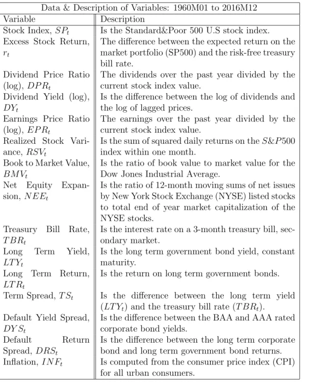
3.1 Data & Description of Variables: 1960M01 to 2016M12 . . . 126
3.2 Descriptive Statistics for the Time Series Variables:1960M01 to 2016M12 . . . 127
3.3 The Statistical and Economic Performance Evaluation Results . . . 130
3.4 The Statistical and Economic Performance Evaluation Results Con-tinued . . . 131
4.1 The Activation Functions . . . 170
4.2 Data & Description of Variables:1960M01 to 2016M12 . . . 173
4.3 Statistical and Economic Performance: 1981M1 to 2016M12: TOOS = 432 . . . 175
4.4 Statistical and Economic Performance: 1991M1 to 2016M12: TOOS = 312 . . . 176
4.5 Statistical and Economic Performance: 2001M1 to 2016M12: TOOS = 192 . . . 177
List of Figures
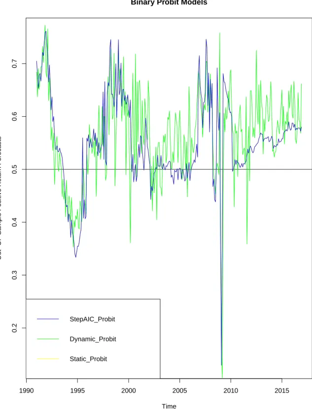
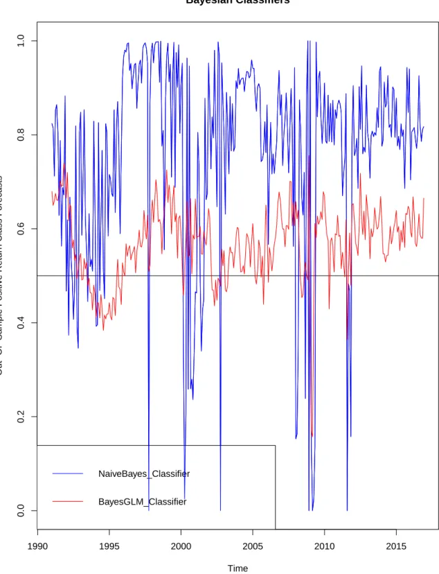
2.1 Graphical Representation of the Out-of-Sample Positive Class
Re-turn Forecasts . . . 68
2.2 Graphical Representation of the Out-of-Sample Positive Class
Re-turn Forecasts continued . . . 69
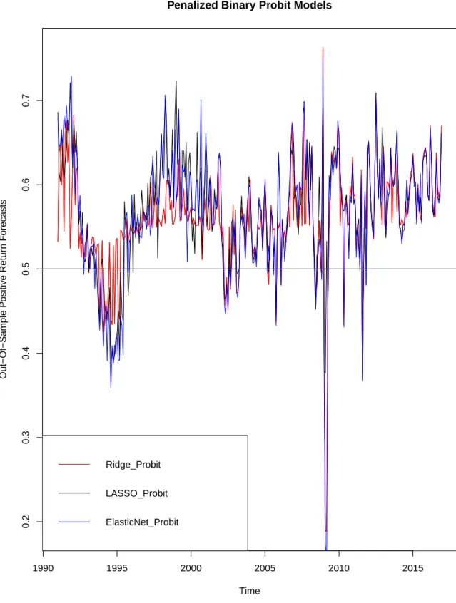
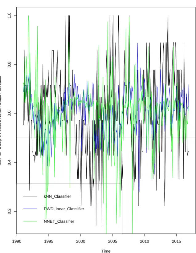
2.3 Graphical Representation of the Out-of-Sample Positive Class
Re-turn Forecasts . . . 70
2.4 Graphical Representation of the Out-of-Sample Positive Class
Re-turn Forecasts continued . . . 71
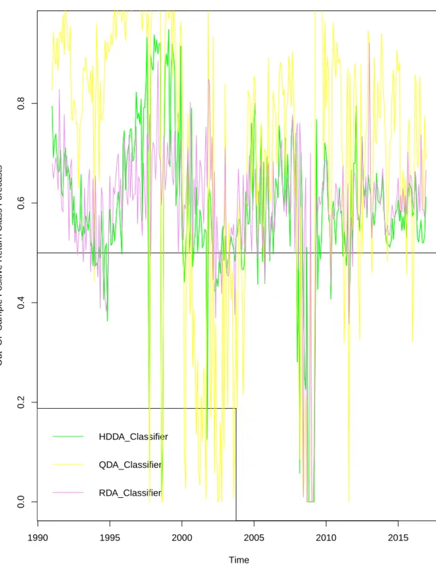
2.5 Graphical Representation of the Out-of-Sample Positive Class
Re-turn Forecasts continued . . . 72
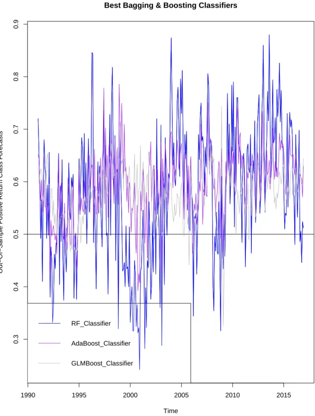
2.6 Graphical Representation of the Out-of-Sample Positive Class
Re-turn Forecasts continued . . . 73
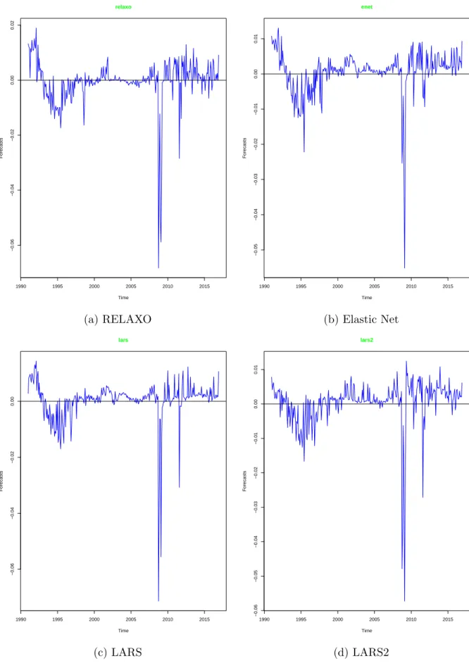
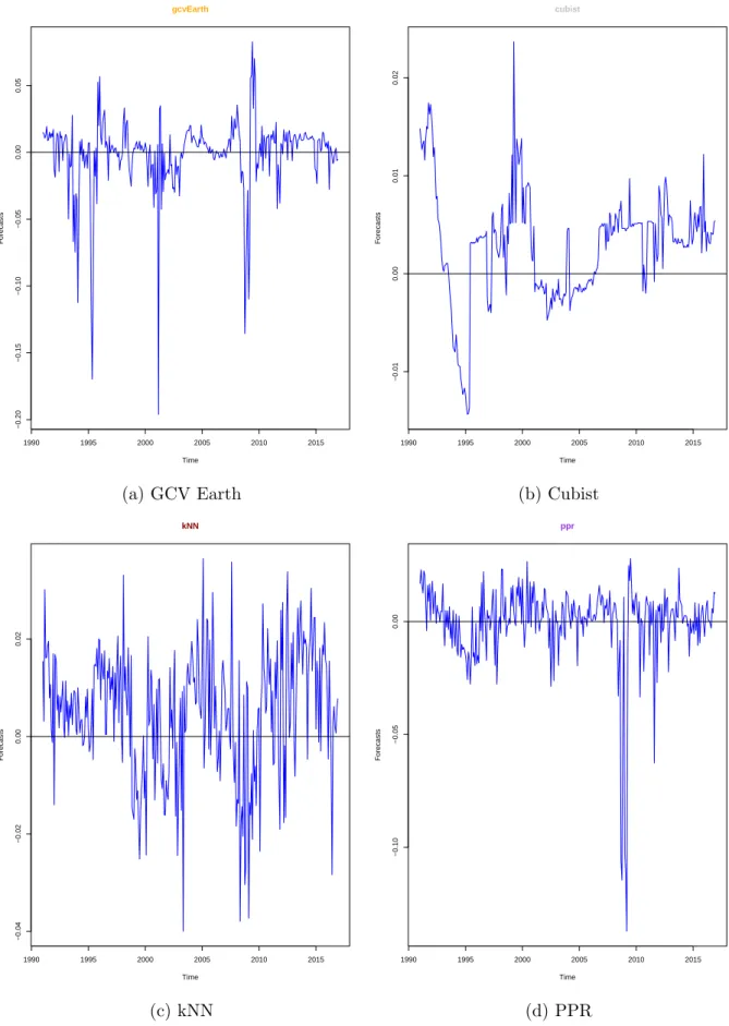
3.1 Out-of-Sample U.S Monthly Equity Premium Forecasts produced
by the RT Models . . . 135
3.2 Out-of-Sample U.S Monthly Equity Premium Forecasts produced
by the RT Models (Continued) . . . 136
3.3 Out-of-Sample U.S Monthly Equity Premium Forecasts produced
by the RT Models (Continued) . . . 137
3.4 Out-of-Sample U.S Monthly Equity Premium Forecasts produced
by the RT Models (Continued) . . . 138
3.5 Out-of-Sample U.S Monthly Equity Premium Forecasts produced
3.6 Out-of-Sample U.S Monthly Equity Premium Forecasts produced
by the RT Models (Continued) . . . 140
3.7 Out-of-Sample U.S Monthly Equity Premium Forecasts produced
by the RT Models (Continued) . . . 141
3.8 Out-of-Sample U.S Monthly Equity Premium Forecasts produced
by the RT Models (Continued) . . . 142
3.9 Out-of-Sample U.S Monthly Equity Premium Forecasts produced
by the RT Models (Continued) . . . 143
3.10 Difference in benchmark historical average forecast cumulative square prediction error and the individual RT model forecast cumulative square prediction error (DCSPE) . . . 144 3.11 Difference in benchmark historical average forecast cumulative square
prediction error and the individual RT model forecast cumulative square prediction error (DCSPE) continued . . . 145 3.12 Difference in benchmark historical average forecast cumulative square
prediction error and the individual RT model forecast cumulative square prediction error (DCSPE) continued . . . 146 3.13 Difference in benchmark historical average forecast cumulative square
prediction error and the individual RT model forecast cumulative square prediction error (DCSPE) continued . . . 147 3.14 Difference in benchmark historical average forecast cumulative square
prediction error and the individual RT model forecast cumulative square prediction error (DCSPE) continued . . . 148 3.15 Difference in benchmark historical average forecast cumulative square
prediction error and the individual RT model forecast cumulative square prediction error (DCSPE) Continued . . . 149 3.16 Difference in benchmark historical average forecast cumulative square
prediction error and the individual RT model forecast cumulative square prediction error (DCSPE) Continued . . . 150
3.17 Difference in benchmark historical average forecast cumulative square prediction error and the individual RT model forecast cumulative square prediction error (DCSPE) Continued . . . 151 3.18 Difference in benchmark historical average forecast cumulative square
prediction error and the individual RT model forecast cumulative square prediction error (DCSPE) Continued . . . 152
4.1 Out-of-Sample U.S Monthly Equity Premium Forecasts by Deep
Learning Models: January 1981 to December 2016 . . . 180
4.2 Out-of-Sample U.S Monthly Equity Premium Forecasts by Deep
Learning Models: January 1981 to December 2016 (continued) . . . 181
4.3 Out-of-Sample U.S Monthly Equity Premium Forecasts by Deep
Learning Models: January 1981 to December 2016 (continued) . . . 182
4.4 Out-of-Sample U.S Monthly Equity Premium Forecasts by Deep
Learning Models: January 1991 to December 2016 . . . 183
4.5 Out-of-Sample U.S Monthly Equity Premium Forecasts by Deep
Learning Models: January 1991 to December 2016 (continued) . . . 184
4.6 Out-of-Sample U.S Monthly Equity Premium Forecasts by Deep
Learning Models: January 1991 to December 2016 (continued) . . . 185
4.7 Out-of-Sample U.S Monthly Equity Premium Forecasts by Deep
Learning Models: January 2001 to December 2016 . . . 186
4.8 Out-of-Sample U.S Monthly Equity Premium Forecasts by Deep
Learning Models: January 2001 to December 2016 (continued) . . . 187
4.9 Out-of-Sample U.S Monthly Equity Premium Forecasts by Deep
Abstract
Conventional market theories are considered to be inconsistent approach in mod-ern financial analysis. This thesis focuses mainly on the application of sophisti-cated machine learning and deep learning techniques in stock market statistical predictability and economic significance over the benchmark conventional efficient market hypothesis and econometric models. Five chapters and three publishable papers were proposed altogether, and each chapter is developed to solve specific identifiable problem(s).
Chapter one gives the general introduction of the thesis. It presents the state-ment of the research problems identified in the relevant literature, the objective of the study and the significance of the study. Chapter two applies a plethora of machine learning techniques to forecast the direction of the U.S. stock mar-ket. The notable sophisticated techniques such as regularization, discriminant analysis, classification trees, Bayesian and neural networks were employed. The empirical findings revealed that the discriminant analysis classifiers, classification trees, Bayesian classifiers and penalized binary probit models demonstrate signif-icant outperformance over the binary probit models both statistically and eco-nomically, proving significant alternatives to portfolio managers. Chapter three focuses mainly on the application of regression training (RT) techniques to fore-cast the U.S. equity premium. The RT models demonstrate significant evidence of equity premium predictability both statistically and economically relative to the benchmark historical average, delivering significant utility gains. Chapter four investigates the statistical predictive power and economic significance of financial stock market data by deep learning techniques. Chapter five give the summary,
conclusion and present area(s) of further research.
The techniques are proven to be robust both statistically and economically when forecasting the equity premium out-of-sample using recursive window method. Overall, the deep learning techniques produced the best result in this thesis. They seek to provide meaningful economic information on mean-variance portfolio in-vestment for investors who are timing the market to earn future gains at minimal risk.
Dedication
This doctoral thesis is dedicated to my lovely wifeMrs. Joy Uzoamaka Iworiso,
a virtuous woman with honour and integrity. She stood firmly with me from the beginning to the end of this terminal degree programme regardless of the distance as young couples. Our love will remain fresh, waxing stronger and stronger, from grace to greater grace till Jesus comes.
Acknowledgements
My profound gratitude goes to God Almighty for his love, faithfulness, mercy, protection and provision throughout this PhD programme. May his name be glo-rified forever.
I wish to express my heartfelt gratitude to the Federal Government of Nigeria for counting me worthy among millions of Nigerians to fund my PhD degree pro-gramme in the United Kingdom.
Suffice it to say that a research has never been successful without a laid-down direction, may I express my sincere appreciation to my amiable and distinguished
supervisor Dr. Spyridon Vrontos for painstakingly supervising my PhD
re-search. His constructive criticisms and suggestions contributed immensely to boost my academic status as doctoral scholar to face the task ahead.
Finally, I am grateful to all persons who have contributed in one way or the other to the success of this achievement.
List of Publications
The first paper (chapter 2 of this thesis) is published in a reputable international journal. The second and third papers (chapters 3 and 4 of this thesis) have been submitted for publication, and are currently on peer review.
1. Iworiso, J. & Vrontos, S. (2019). On the Directional Predictability of Equity Premium Using Machine Learning Techniques. Journal of Forecasting, 1-21. https://doi.org/10.1002/for.2632
2. Iworiso, J. & Vrontos, S. (2019). Forecasting the U.S. Equity Premium with Regression Training Techniques. Journal of Empirical Finance. Unpublished (peer review in progress).
3. Iworiso, J. & Vrontos, S. (2019). On the Predictability of Equity Premium Using Deep Learning Techniques. International Journal of Forecasting. Un-published (peer review in progress).
Chapter 1
Introduction
A notable quest in modern financial literature is the search for more suitable mod-els that can explicitly model and forecast financial time series data with utmost precision to guarantee investors future expectation at extremely low volatility. In this case, the researchers are expected to present models that can significantly outperformed the conventional financial modelling and forecasting approach. A number of statistical and econometric models have been applied by various schol-ars over the yeschol-ars. Although the empirical findings in most situations are proven to outperformed the conventional approaches but are generally considered to be weak as compared to a rule of thumb (i.e., at least 50%) especially in sign forecast-ing and market dynamics (Leitch and Tanner, 1991; Christoffersen and Diebold,
2006; Anatolyev and Gospodinov, 2010; P¨onk¨a, 2016), and hence, the need for
further research in this field of study. The empirical findings in Nyberg (2011, 2013) demonstrates the effectiveness of static and dynamic statistical models in fi-nancial time series analysis but the resulting predictive power of the models seems to be weak and required further statistical and economic performance evaluation measures to affirm the stability in finance. The classification and level estimation techniques in Leung et al. (2000) greatly provides evidence of useful predictabil-ity over the conventional financial methodologies known as the benchmark buy and hold (B&H) trading strategy, with the discriminant classifier emerging as the superior model in this perspective. The quest for a superior model to forecast
equity risk premium out-of-sample comparative to the benchmark historical av-erage with convincing statistical and economic performance evaluation measures to a mean-variance portfolio investor, is another crucial debatable research issue in modern finance (Goyal and Welch, 2003; Campbell and Thompson, 2005, 2007; Rapach et al., 2007; Neely et al., 2014; Baetje and Menkhoff, 2016; Bai, 2010; Li and Tsiakas, 2017). Although the statistical and econometric models used in the afore-mentioned studies demonstrate feasibility and evidence of both statistically and economically significant predictability but further investigation is required to authenticate the fate of investors timing the market to maximize profit at minimal risk.
The earnest expectation of the stock market outcome to mean-variance in-vestors above the treasury bill rate led to the quest for a meaningful estimate of excess stock return or equity premium (Campbell, 2008). The equity premium is the difference between the expected return on the market portfolio (SP500) and the risk free interest rate. Thus, investors can expect this return from holding the market portfolio in excess of the return on the 3-month Treasury bills. It is considered to be the most crucial concept in finance, owing to portfolio alloca-tion decisions and cost of capital estimates. It is worth noting that the backbone of investment strategies depends on the ability to predict future returns but the predictability itself does not necessarily guarantee the investor’s profit from the trading strategy based on the resulting forecasts (Campbell and Thompson, 2005; Bai, 2010). An academic debating question in modern review of financial studies is that: can any other model accurately forecast the equity premium better than the forecasts from the historical average? Goyal and Welch (2007) have argued that no other variable beats a simple forecast based on the historical average, and concluded that the in-sample correlations conceal a systematic failure of the finan-cial and economic variables out-of-sample. Contrary to this empirical analysis, the results in Rapach et al. (2007) reveals that despite the failure of the individual model forecasts to outperform the historical mean forecasts, the combination of
the individual model forecasts yield statistically and economically significant gains, relative to the historical mean, consistently over time. Although some of the in-dicators used as predictors appeared to be good statistically significant predic-tors of the equity premium in-sample at some specific horizons but are relatively poor in the out-of-sample forecasting ability. Fama and French (2002) verified that the estimates from economic fundamentals especially in the dividend growth model, appeared to produce lower standard errors resulting to corresponding bet-ter precision than the estimates from the benchmark historical average model. The combination approach in Neely et al. (2014) confirmed that both technical indicators and macroeconomic variables displayed statistically and economically significant evidence of in-sample and out-of-sample forecasting ability, with the technical indicators seemingly outperforming the macroeconomic variables. The empirical analysis suggests that the combination of both technical indicators and macroeconomic variables will significantly improve the equity risk premium fore-casts rather than using a single set of the predictor variables alone. However, the findings require further investigation for either corroboration or refutation. Following this argument, Baetje and Menkhoff (2016) demonstrated that the pre-dictive abilities of both indicators seem to possess similar quality when assessed by their respective long term forecast errors. Unlike the economic indicators that loses predictive ability on a long run, the technical indicators maintain or increase stability over time, and hence, the technical indicators consistently outperformed the economic indicators over time. The application of forecasts combination in Rapach et al. (2010) confirmed that combination of forecasts yields statistically and economically significant out-of-sample gains consistently on a long run, com-pared to the benchmark historical average. Therefore, the forecasts combination approach in Rapach et al. (2010) appeared to maintain a long run statistical and economic stability.
However, evaluating the mean squared errors (MSEs) and Sharpe ratios (SRs) alone, do not provide adequate evidence to justify the superiority of a specific
model over other competitive models. Some existing papers focused mainly on evaluating the model prediction errors, expected returns on portfolio investment and the corresponding Sharpe ratio. In addition to these parametric measures, Ny-berg (2011) included the Diebold-Mariano (DM) statistical tests and the Pesaran-Timmermann (PT) directional predictability tests only in the in-sample case, but do not investigate the DM among the models in the out-of-sample case. The benchmark used in the study was the expected return on a portfolio investment held on a risk-free interest rate, based on the buy and hold trading strategy. Goyal and Welch (2003), Campbell and Thompson (2005) were mainly concerned with examining the predictive ability of individual predictor variables relative to the benchmark historical average, using the out-of-sample statistical goodness of fit
tests and the SRs, whereas Campbell and Thompson (2007); Campbell (2008),
Goyal and Welch (2007) and Rapach et al. (2010) added an important concept
known as theutility gain, which serves as an additional benchmark for comparing
the economic performance of a model to a portfolio investor with a portfolio held on the risk-free Treasury bill. However, some important concepts such as cumu-lative returns among others were not included in their studies. It is imperative to explore adequate statistical predictive and economic significance tests especially in the out-of-sample forecasting models, to determine superiority among the resulting models used in the study.
In modern research, the use of machine learning and deep learning techniques is drawing rapid attention in financial time series analysis. Machine learning is the study of sophisticated algorithms and mathematical models existing between input features and target output or to learn and recognize patterns in order to improve the performance on a specific task typically by computer systems. In this case, the algorithm builds a model from sample training data and use the resulting model to make predictions without being explicitly programmed to perform the specific task. The feasibility of some machine learning techniques in finance (Kumar and Thenmozhi, 2006; Chen, 2011; Huang and Wu, 2008; Ince and Trafalis, 2007;
Pahwa et al., 2017; Patel et al., 2015) with desirable predictive performance had
led to the introduction of more sophisticated learning technique known as deep
learning which have the ability to extract features from a large raw dataset without
relying on prior knowledge of predictors. Day and Lee (2016) described deep
learning as deep neural network, which is a more sophisticated aspect of machine learning. It is a form of machine learning technique that involved the use of data to train a model or recognize pattern(s) or label instances in order to make predictions from new data in a more sophisticated manner (Heaton et al., 2017). Machine learning and deep learning techniques are shown in empirical literature to be useful techniques to learn data, recognize patterns such as speech recognition, and to classify instances such as digital image classification. They appeared to be useful modern research techniques for analysis in computer science, biology, medicine, linguistics, physics, statistics, economics and finance.
It is worth noting that the machine learning algorithms/models introduced in financial and econometric literature do not provide adequate statistical predictive and economic significant measuring tools for comparing their performances with the conventional efficient market hypothesis and econometric models. Suffice it to say that the justification of a predictive model in terms of superiority over the conventional models in finance depends on both statistical and economic perfor-mance measures. The findings in Kumar and Thenmozhi (2006), Chen (2011) and Chen and Hao (2017) are promising, but do not provide adequate statistical and economic measures to demonstrate the superiority of machine learning tech-niques over the benchmark approaches in finance. Yoshihara et al. (2014) shows that recurrent deep neural networks appeared to be more effective approach over
support vector machines (SV M) and deep belief networks when predicting the
trend of stock market, especially when the process is focused on specific period after a known significant event in financial domain. The analysis provides a con-troversial superiority of recurrent neural networks over the deep belief network in this direction. The empirical findings in (Zhao et al., 2017) shows the
superior-ity of deep learning ensemble with stacked denoising autoencoders for modelling and forecasting crude oil prices over the bootstrap aggregation and other ma-chine learning techniques used in the literature. The empirical results in Hu et al. (2018), Feuerriegel and Fehrer (2016), Heaton et al. (2016) also confirmed that the application of deep learning techniques in financial analysis seek to outperformed both the standard methods in finance and the conventional machine learning tech-niques. Armano et al. (2005) introduced a hybrid genetic-neural architecture to forecast stock indexes with consideration of realistic trading commission, and ap-peared to be promising in the selected application task. The empirical findings also demonstrate evidence of superior outperformance over the benchmark buy and hold strategy for a large test sample size. Contrary to these analyses, is the empirical results in Krauss et al. (2017) in which a random forest outperformed some notable deep learning techniques. It was shown that the random forest out-performed both deep neural networks (DNN) and gradient boosted trees in the investigation of statistical arbitrage on SP500, and concluded that a further inves-tigation by hyper-parameter optimization for the deep neural networks is required as an area of future research work.
The statement of the problem lies on the provision of superior technique that can significantly outperform the existing conventional econometric models and to fill the identifiable research gaps in the existing literature. The objective of this study is to explore the sophisticated machine learning and deep learning techniques to model financial stock market data in order to make predictions and evaluate their performances with robustness, and to demonstrate superior outperformance of these proposed methodologies in the thesis over the benchmark approaches used in the existing literature. The study aimed to introduce additional statistical and economic performance evaluation measures that can authenticate the long-run effectiveness and consistency of the proposed models in relation to optimistic in-vestment approach for yielding future gains. Therefore the outcome of this study shall provide significant statistical and economic information to stock market
in-vestors and portfolio managers on the need for optimal portfolio assessment with a view to maximize profit at minimal risk when timing the market. It shall also fill the identifiable research gaps, enrich empirical literature and present area of further research to future researchers on the subject matter.
Chapter 2
Directional Predictability of U.S.
Stock Market Using Machine
Learning Techniques
2.1
Introduction
Stock market participants aim at maximising returns on portfolio investments at minimal risk. Consequently, forecasting stock market returns has received con-siderable attention in recent years. The majority of papers have focused on the forecast accuracy of competing models and examined if there is evidence of pre-dictability, which can lead to economic gains. However, devising successful trading strategies is contingent on the directional accuracy of the underlying models. The literature on directional predictability is sparse, and the empirical findings offer limited support. For example, the findings in (Chevapatrakul, 2013; Christoffersen
and Diebold, 2006; Nyberg and P¨onk¨a, 2016) provide weak evidence of directional
stock market predictability. Although the predictive power of the models em-ployed so far are shown to be weak in statistical terms, they seem to provide economic value. Thus, the emphatic challenge lies in the development of a suit-able directional predictive model involving the relevant financial and economic variables.
The application of some benchmark econometric models used in previous find-ings are shown to be weak in terms of predictive performance. The introduction of recursive and alternative rolling windows out-of-sample estimation and forecasting
techniques used by Nyberg (2008, 2011), P¨onk¨a (2016) provide statistically
sig-nificant evidence of the directional predictability of stock market returns, but the predictive power of the models are shown to be relatively weak, and hence, there is a need to introduce sophisticated machine learning techniques, as proposed in this study to improve the predictive task of the models.
This chapter focuses on the application of sophisticated machine learning tech-niques on binary probit and classification models to forecast the direction of the U.S. excess stock market returns. The machine learning techniques employed in-clude classification and regression trees (CART), such as Bagging, Boosting and Discriminant Analysis classifiers, Bayesian classifiers, Neural Networks and reg-ularization techniques, such as Ridge, Least Absolute Shrinkage and Selection Operator (LASSO), and Elastic Net. To compare our findings with the previous literature, we also include four variants of the benchmark binary probit models, namely, the static, stepwise static, dynamic and stepwise dynamic models. The application of CART forecasting models aims to explore all covariates as ensem-bles to learn the data, train the classification model, recognize patterns, classify instances and to forecast future binary outcomes. With respect to penalised binary probit models, it is important to note that the presence of shrinkage penalty vec-tor norms could result to a bias in coefficient estimates, reduction in the forecast errors and improvement in predictive performance via the so-called bias-variance trade off. Thus, the proposal of CART and penalized predictive models in this chapter aims at yielding superior statistical predictive performance and economic significance compared to the benchmark econometric models typically employed in the literature to date.
2.2
Literature Review
A notable quest in modern financial econometric literature is the application of suitable techniques to predict the sign of stock market returns. A review of rele-vant empirical literature has revealed that the use of econometric models for the directional predictability of excess stock returns are known to produce weak pre-dictive power, poor statistical goodness of fit and low prepre-dictive accuracies, among others; see (Pesaran and Timmermann, 1995; Nyberg, 2011; Leung et al., 2000;
Chevapatrakul, 2013; Leitch and Tanner, 1991; P¨onk¨a, 2016), even though the
empirical results seems to provide economic significance.
The previous findings on directional predictability by Anatolyev and Gospodi-nov (2010), and Hong and Chung (2003) have employed a logistic regression model to predict the sign of U.S. stock market returns using relevant financial vari-ables as the key predictors, and their results provide evidence of predictability, but the overall predictive power is relatively weak, compared to a rule of thumb (i.e., at least 50%). In an attempt to determine market timing and asset allo-cation decisions between stocks and risk-free assets, some researchers considered the role of conditional mean and volatility while predicting the sign of asset re-turns. Christoffersen and Diebold (2006) have opined that the direction of asset returns is predictable, as volatility dependence produces sign dependence, so long as expected returns are nonzero. This notion seems to be true, as other existing papers have also provided significant statistical evidence of the sign predictability of the U.S. stock market returns and economic recession status by application of static, dynamic, autodynamic and error correction models, both in-sample and
out-of-sample (Nyberg, 2011; Kauppi and Saikkonen, 2008; Nyberg and P¨onk¨a,
2016; Nyberg, 2013).
The static and dynamic probit models proposed by Nyberg (2011) to predict the direction of monthly U.S. excess stock returns recursively appears to have out-performed the autoregressive moving average with exogenous inputs models (AR-MAX), vector autoregressive-generalized autoregressive conditional
heteroskedas-ticity (VAR-GARCH) models, etc. used by previous researchers. The idea was based on the approach used by Kauppi and Saikkonen (2008), Estrella and Mishkin (1998) to obtain U.S. economic recession forecasts using variables such as the U.S. term spread and lagged stock returns, among others.
However, according to the Nyberg (2011) paper, the Estrella’s statistical good-ness of fit values in the various probit models are very low in all cases. The positive values of the Sharpe ratios signified that investors are likely to have positive re-turns on portfolio investments. The percentage of correct matches as a statistical performance evaluation measure in the existing papers are relatively low, hence the need to employ more advanced sophisticated models that can yield a better degree of accuracy with the smallest prediction error.
The underlying challenges associated with the use of financial and economic variables to predict stock market returns has prompted researchers to introduce sophisticated statistical or machine learning algorithms to improve the predic-tive task and the overall performance of the resulting models under consideration. It is noticeable from the empirical literature that machine learning techniques, which include Random Forest, Linear Discriminant Analysis (LDA), k-Nearest Neighbour, Tree-based Classification, Recursive Partitioning, Bagging and Boost-ing, Logistic Regression, Support Vector Machine (SVM), Ridge Regression, Least Absolute Shrinkage and Selection Operator (LASSO), Least Angle Regression and Elastic Nets, are useful for the analysis of financial econometric time series (Roy et al., 2015; Sermpinis et al., 2017; Li and Chen, 2014; Inoue and Kilian, 2008; Zhou et al., 2015; Hsu et al., 2008; Park and Sakaori, 2013; Chen, 2016; Stock and Watson, 2012; Lin and McClean, 2001; Kim and Swanson, 2014; Hajek et al., 2014; Shen et al., 2014; Pahwa et al., 2017; Swanson and White, 1997). Khaidem et al. (2016) used the Random Forest method to predict the direction of stock market prices. The algorithm appears to be robust in predicting the future direction of the stock market movement, thus minimizing the risk of investment in the stock market with good predictive accuracy.
The ridge regression introduced by Hoerl and Kennard (1970), and the least ab-solute shrinkage and selection operator (LASSO) introduced by Tibshirani (1996) are found to be useful statistical or machine learning techniques for econometric models. The ridge regression reduces multicollinearity and minimizes the model prediction error but does not perform feature selection; the LASSO shrinks the model coefficients towards zero and performs feature selection and model inter-pretability. The aim is to introduce bias in the model coefficient estimates and minimize the prediction error.
The empirical analysis in Inoue and Kilian (2008) revealed that bagging has large reductions in prediction mean square errors (PMSEs) in inflation forecast-ing. Kim and Swanson (2014) suggest that the model averaging does not dominate other well designed prediction model specification methods, and that the use of hybrid combination factor and shrinkage methods produced the best predictions as compared to principal components, bagging, boosting, least angle regression, among others. On the other hand, the empirical results from Zhou et al. (2015) showed no statistically significant difference between the best classification perfor-mance of the models with yearly feature selection guided by data mining techniques and the one involving domain knowledge; hence, their predictive accuracies seems to be the same.
The use of the LASSO linear regression model for stock market forecasting in Roy et al. (2015) using monthly data revealed that the LASSO method yield sparse solutions and performs extremely well when the number of features is less than the number of observations, and that the LASSO linear regression model outperforms the ridge linear regression model. Modelling the market implied rat-ings using LASSO variable selection techniques in Sermpinis et al. (2017) and forecasting macroeconomic time series using LASSO-based approaches and their forecast combinations with dynamic factor models in Li and Chen (2014) all reflect statistical evidence of the superior predictive power of LASSO.
tech-niques over the benchmark econometric and statistical modelling techtech-niques has prompted modern researchers to proceed into a more advanced concept, i.e., the deep learning techniques based on artificial intelligence, which encompasses sup-port vector machines (SVM) and neural networks (NNET). However, the con-trasting arguments of various scholars on the predictive performance by SVM and NNET as compared to the previous literature has placed this notion pending for further statistical investigation. The application of artificial neural networks (ANN) in forecasting financial markets and stock prices in Shahpazov et al. (2014) demonstrated the outperformance of the NNET over previous techniques used in the existing literature. Again, the findings in de Oliveira et al. (2013) also revealed that the application of artificial neural networks yielded the minimum mean square prediction error (MSE) and correct direction rates. Controversially, the analytical results by Moreno and Olmeda (2007) show that the ANN do not provide evi-dence of superior performance over the conventional linear models. The findings in Ding et al. (2013), applying the concept for daily data and market sentiment, shows the outperformance of SVM over NNET and logistic regression. The SVM seems to be the most accurate machine learning model for predicting stock market movement, but the statistical tests do not provide significant statistical evidence of better performance over NNET and logistic regression. Patel et al. (2015) con-firmed the outperformance of Random Forest over ANN, SVM and the genetic algorithm (GA) for input data with continuous values. Ballings et al. (2015) also presented random forest as the top machine learning algorithm over others and recommended the inclusion of ensembles in algorithmic sets when predicting the direction of stock market prices. The findings in Zheng (2006) demonstrated the superiority of boosting and bagging of NNET over SVM and logistic regression when forecasting the daily directional movements of stocks.
It is obvious, based on the reviewed existing empirical literature, that machine learning techniques played an enormous role in financial econometric time series. Thus, the application of the proposed sophisticated machine learning recursive
out-of-sample forecasting models for the directional predictability of the U.S. stock market returns in this paper aimed to yield significant results and outperform the benchmark econometric models and aimed to enrich the empirical literature for further relevant scholarly research work.
2.3
Research Methodology
This section gives a detailed theoretical approach to excess stock return modelling as a binary time series, the static and dynamic binary probit forecasting models; the application of machine learning techniques which include the Ridge, LASSO and Elastic Net probit models; the classification and regression trees (CART); fol-lowed by the forecasting/predictive model performance evaluation for easy com-parison.
2.3.1
Equity Premium Direction Modelling as a Binary
Time Series
Let Rt be the monthly U.S. excess stock market return over the risk-free interest
rate denoted by rft, and let Its denote the binary-valued dependent variable. The
sign of the monthly equity premium is modelled as the return sign binary indicator, as follows: Its=
1, if Rt>0 i.e., positive excess stock market return
0, if Rt≤0 i.e., negative or zero excess stock market return.
(2.1) Rt is calculated as follows: Rt= ln Pt Pt−1 −rft−1 (2.2)
where Pt is the price of the stock index at period t and rft−1 is the risk-free
of the return sign binary indicator Is
t conditional on <t−1 follows Bernoulli with
probability pt, as follows:
Its|<t−1 ∼Bernoulli(pt),
where <t−1 is the information set of the covariates.
2.3.2
The Static and Dynamic Binary Probit Models
Christoffersen and Diebold (2006) showed that if Rt is distributed as follows:
Rt|<t−1 ∼N(µ, σ2t|t−1)
and displays no conditional mean dependence and conditional variance depen-dence, then there exists a link between the volatility dynamics and the sign dynamics. The conditional probability of a positive excess stock market return
P robt−1(Rt>0) is as follows: P robt−1(Rt >0) = 1−Γ −µ σt|t−1 = Γ µ σt|t−1
where Γ(.) is the N(0,1) cumulative distribution function, and the forecast
hori-zon used is equal to 1. The sign of equity premium is predictable if the conditional
probability of positive equity premium P robt−1(Rt > 0) > 0.5 for a threshold of
0.5, varies with the information set <t−1, which invariably implies a direction of
change in the forecastability or predictability of the equity premium (Chevapa-trakul, 2013).
Given the conditional expectation Et−1, conditional on the information set
the binary probit indicator Is
t = 1 is as follows:
pt =Et−1(Its) = P robt−1(Its = 1) =P robt−1(Rt>0) = Γ(Ψt)
where Γ(.) is a standard normal cumulative distribution function.
The static and dynamic binary probit models can be obtained from this direction, using the fact that the autocorrelation between any two successive numerical values of the equity premium is statistically negligible.
Thus, the static binary probit forecasting model is defined as follows:
Ψt+1(β) =α+Z0tβ (2.3)
where α is the model intercept;
Zt isk-dimensional covariate vector of predictors of equity premium;
β isk×1 vector of unknown coefficients (Nyberg, 2011; Nyberg and P¨onk¨a, 2016).
Using the uncorrelated assumption Cor.(Its+1, Its) = 0, the historical value
of the equity premium sign indicator Is
t is included in the static binary probit
forecasting model, which results to the dynamic binary probit forecasting model. Thus, the dynamic binary probit forecasting model is
Ψt+1(β) =α+ p X i=1 ηiIts+Z 0 tβ (2.4)
where α is the model intercept;
η is an unknown coefficient of the lagged equity premium sign indicator;
Zt isk-dimensional covariate vector of the predictors of equity premium;
β isk×1 vector of unknown coefficients;
p is the lag order of the equity premium sign indicator (Kauppi and Saikkonen,
2008).
on the link function:
P rob(Its+1 = 1|<t) = Γ(α+Z0tβ) (2.5)
and the benchmark forecasts from the dynamic binary probit model are based on the link function:
P rob(Its+1 = 1|<t) = Γ(α+ p X i=1 ηiIts+Z 0 tβ) (2.6)
where p≥1 is the lag order (Kauppi and Saikkonen, 2008).
2.3.2.1 Stepwise Variable Selection using Akaike Information
Crite-rion
The stepwise variable selection is a step-by-step selection technique which seeks to screen the predictive variables of a specific model by an automatic iterative pro-cedure. It involves a screening process in that in each step, a predictor variable is considered for inclusion or elimination from the set of predictor variables based on the significant status determined by an information criterion. In this study, the bidirectional (forward-and-backward) stepwise approach with the Akaike in-formation criterion (StepAIC) was used for further investigation of the static and dynamic binary probit models.
2.3.2.2 Likelihood Estimation of Binary Probit Model Parameters
The parameters of the binary probit models defined in (2.3) and (2.4) can be estimated by maximum likelihood method. Given the function:
The likelihood function of β is defined as follows: L(β) = Y (Is t+1=1) ΓΨt+1(β) Y (Is t+1=0) 1−Γ Ψt+1(β) (2.8)
The log-likelihood function is defined as follows:
lnL(β) = X (Is t+1=1) ΓΨt+1(β) + X (Is t+1=0) 1−Γ Ψt+1(β) (2.9)
Thus, the maximum likelihood estimator (MLE) of β is obtained as follows:
ˆ βM L= arg max β X (Its+1=1) Γ Ψt+1(β) + X (Its+1=0) 1−Γ Ψt+1(β)
where Γ(.) is the standard normal cumulative distribution function (Estrella and
Mishkin, 1998; Pesaran, 2015; Kedem and Fokianos, 2005)
2.3.3
The Penalized Binary Probit Models for Stock
Re-turn Predictability
This section examined the penalized likelihood binary probit models employing the relevant Ridge, LASSO and Elastic Net structures. The inclusion of a penalty vector norm in the log-likelihood function of the ordinary binary probit model results in the penalized binary probit model. It is worth noting that in the penal-ized likelihood binary probit models, the coefficient estimates are shrunk towards zero. The regularized biased coefficients are known to have significantly reduced variances, that could result in smaller forecasting errors.
2.3.3.1 The Ridge Binary Probit Model
The ridge binary probit model aims to reduce multicollinearity and minimize the prediction error of the model and is based on the ridge regression introduced by Hoerl and Kennard (1970). Given the log-likelihood function of the ordinary binary probit model (2.9), the ridge log-likelihood probit function introduces a
penalty on the `2-norm of β:
lnL(βλ) = X (Its+1=1) Γ Ψt+1(β) + X (Its+1=0) 1−Γ Ψt+1(β) −λ k X j=1 βj2 =lnL(β)−λkβk22 (2.11)
wherelnL(β) is the unrestricted log-likelihood function of the probit model;kβk22 =
q
Pk
j=1βj2 is the `2-vector norm of β; λ >0 is the ridge tuning parameter which
controls the amount of regularization of the norm ofβ.
Thus, the maximum likelihood estimator of the ridge binary probit model is given by the following: ˆ βRM LEλ = arg max β X (Is t+1=1) ΓΨt+1(β) + X (Is t+1=0) 1−Γ Ψt+1(β) −λ k X j=1 βj2
where ˆβλ is the maximizer of the ordinary probit model.
2.3.3.2 The LASSO Binary Probit Model
The Least Absolute Shrinkage and Selection Operator (LASSO) introduced by Tibshirani (1996) as a shrinkage and selection technique for linear regression mod-els is extended to binary probit modmod-els. The proposed LASSO binary probit model aims to shrink the probit model coefficients toward zero, yielding bias parameter estimates, resulting in the model interpretability and identification of the covari-ates most strongly associated with the equity premium direction.
function of the ordinary binary probit model (2.9) will include a shrinkage penalty
on `1-norm of β. The introduction of the constraint into the probit model is
ex-pressed by incorporating a shrinkage penalty to the log-likelihood of the model. Thus, the constraint maximization for the log-likelihood becomes:
lnL(βλ) = X (Is t+1=1) ΓΨt+1(β) + X (Is t+1=0) 1−Γ Ψt+1(β) −λ k X j=1 |βj|=lnL(β)−λkβk1 (2.12)
wherelnL(β) is the unrestricted log-likelihood function of the probit model;kβk1 =
q
Pk
j=1|βj| is the `1-vector norm of β; λ > 0 is the LASSO tuning parameter,
which controls the amount of shrinkage (regularization) of the norm of β.
The vector ˆβλ
LM LE, that maximizeslnL(βλ) is the LASSO binary probit estimator
of β, hence, the LASSO binary probit model coefficient estimates are obtained by
ˆ βLM LEλ = arg max β X (Is t+1=1) Γ Ψt+1(β) + X (Is t+1=0) 1−Γ Ψt+1(β) −λ k X j=1 |βj|
where ˆβλ is the maximizer of the ordinary probit model.
2.3.3.3 The Elastic Net Binary Probit Model
The elastic net (EN) is a regularized technique that linearly combines the `1 and
`2 penalties of the LASSO and Ridge. The elastic net probit coefficient estimates
ˆ
βλ,αEM LE are obtained by maximizing the log-likelihood function, which penalized
the size of the model coefficients based on both the `1-vector norm and `2-vector
norm of β, defined by the following:
lnL(βλ,α) = X (Is t+1=1) ΓΨt+1(β) + X (Is t+1=0) 1−Γ Ψt+1(β) −λ(1−α) k X j=1 β2 j 2 +α k X j=1 |βj| (2.13)
Thus, the parameter estimates of the elastic net binary probit model will be given by the following: ˆ βλ,αEM LE= arg max β X (Is t+1=1) ΓΨt+1(β) + X (Is t+1=0) 1−Γ Ψt+h(β) −λ(1−α) k X j=1 β2 j 2 +α k X j=1 |βj|
where λ and α are the elastic net tuning parameters (Zou and Hastie, 2005). In
this study, the penalty factor α = 0.5 was employed, which results to an elastic
net probit model.
To choose the tuning parameters λ, λ1, λ2 in Ridge, LASSO and Elastic Net,
we need a validation set in which the predictive value of the specific penalized bi-nary probit model could be compared for various values of the tuning parameter, and the optimal tuning parameter should be chosen such that the error rate is minimal. In this study, the best tuning parameter employing cross-validation was chosen for each model.
2.3.4
Classification and Regression Trees for Stock Return
Predictability
The concept of classification and regression trees (CART) was first introduced by Breiman et al. (1984), which involves the use of decision tree learning procedures to build a model that can predict the value of a target variable based on several input variables. There are many classification algorithms, including decision trees, rule-based learners, exemplar learners, discriminant functions, neural networks and Bayesian networks, that are considered to be useful in modern forecasting. There are also ways of combining them into ensemble classifiers, such as bagging, boosting, and random forest. The consistent CART models in this study are as
follows:
2.3.4.1 Bagging
Bagging or bootstrap aggregating was introduced in 1994 by Breiman (1996) to improve classification by combining classifications of randomly generated training datasets, to reduce the biases and variances in a tree-based analysis. Bagging im-plies fitting a model, including all potential points on the original training set. It appears to effectively remove the instability of a decision rule by averaging across resamples and to avoid overfitting (Zheng, 2006).
Let S = {(Z1, y1),(Z2, y2), ...,(Zt, yt), ...,(ZT, yT)} denote the training sample,
where T is the number of observations in the training sample, Zt is a vector
ofk covariates, andyt ∈ {−1,1}indicates a positive or negative return for each t.
The classification into one of the two groups is defined as follows:
ˆ
Ψ(Z) =signˆδ(Zt)−τB
,Ψ(Z)ˆ ∈ {−1,1}
where τB is the threshold (cut-off value); ˆδ(Zt) is the base classifier that learned
the covariates in the training sample; ˆδ(Zt)> τB implies a positive return
classi-fication, while ˆδ(Zt) < τB implies a negative return classification (Lemmens and
Croux, 2006).
The decision tree classification score is given by the following:
ˆ
δ(Z) = 2 ˆρ(Z)−1
where ˆρ(Z) is the predicted probability of a positive return estimated by the tree.
For each bootstrap sampleSb∗, b= 1,2, ..., B, a classifier can be estimated assigning
B score functions ˆδ∗1(Z),δˆ2∗(Z), ...,δˆb∗(Z), ...,δˆ∗B(Z).
These functions are afterwards aggregated into a score, as follows:
ˆ δbag(Z) = 1 B B X b=1 ˆ δb(Z)
Thus, the final classification is obtained as follows: ˆ Ψbag(Z) =sign ˆ δbag(Z)−τB ,Ψ(Z)ˆ ∈ {−1,1} (2.14) 2.3.4.2 Random Forest
A random forest (RF) classifier, see Breiman (2001), is a specific type of boot-strap aggregating based on a random subset of the input features (Ballings et al., 2015; Kumar and Thenmozhi, 2006; Creamer, 2009). A random forest classifier consists of an ensemble classification algorithm that involves the use of trees as base classifiers. It consists of a combination of classifiers in which each classifier contributes an individual vote for assigning the most frequent class to the input
vector Z, defined by the following:
ˆ δB RF =majority vote n ˆ δb(Z) oB b=1 (2.15)
where ˆδb(Z) is the class prediction of the bth random forest tree; Z is the input
vector; b= 1,2, ..., B.
The Gini index approach suggested by Breiman et al. (1984) is a suitable measure for selecting the best splits which determines the impurity of a given element with respect to the classes, and hence, it is employed for selecting the best split at each node.
Given a training dataset S, involving a set of covariates and categorical target
outcome, the Gini index can be computed as follows:
I(τ) =X i X j6=i h(δi,S) |S)| h(δj,S)) |S)| (2.16) where h(δi,S))
|S)| is the probability that a selected instance belongs to class δi;
h(δj,S))
|S)| is the probability that a selected instance belongs to class δj; for i 6=
j (Rodriguez-Galiano et al., 2012). Thus the random forest seek to produce a
Alternatively, for a given node τ with estimated class probabilities P rob(j|τ), j = 1, ..., J, the node impurity, I(τ), employing the Gini index is defined as follows:
I(τ) =
J
X
j6=i
P rob(j|τ)P rob(i|τ). (2.17)
The Gini index is minimised when the node is pure (homogeneous) with respect to one of the classes.
2.3.4.3 Conditional Inference Tree
The conditional inference tree (CTree) enables the use of recursive partitioning and tree-structured models in a conditional inference framework. The use of the Gini index to determine the most favourable split induces a selection bias toward covariates with many possible splits and also cannot distinguish between a signifi-cant and an insignifisignifi-cant improvement in the information measure. Hothorn et al. (2006) proposed the conditional inference approach tree where the node split is selected based on how good the association is between the response and the covari-ates. The resulting nodes should provide a high association between the response
and the covariates. The significance of the association is investigated by a χ2 test
and the covariate with highest association is selected for splitting. Moreover, mul-tiple test procedures are applied to determine whether no significant association between any of the covariates and the response can be stated and the recursion needs to stop.
In more detail, let Z = (Z1,· · · , Zk) be the k-dimensional vector of covariates
and let y be a categorical response variable. Z is taken from a sample space
Z = Z1 × · · · × Zk. We assume that the conditional distribution of y given Z
depends on the function f of Z as follows:
Thus, a generic algorithm for recursive binary partitioning for a given learning sample
Ln= (yi, Z1i,· · · , Zki), i= 1,· · · , n,
can be formulated using non-negative integer valued case weightsw= (w1,· · · , wn).
Each node of the tree is represented by a vector of case weights having nonzero elements when the corresponding observations are elements of the node, and are zero otherwise. The following steps implement recursive binary partitioning:
1. Test the global null hypothesis of independence between any covariateZand
the categorical response variableyfor case weightsw. Stop if this hypothesis
cannot be rejected. Otherwise, select the j-th covariateZj with the strongest
association to y.
2. Choose a set A ⊂ Zj to split Zj into two disjoint sets of A and Ac. The
case weights wlef t and wright determine the two subgroups with wlef t,i =
wiI(Zj,i ∈ A) and wright,i = wiI(Zj,i ∈/ A), for all i = 1,2,· · ·, m , where
I(·) is the indicator function.
3. Repeat steps 1 and 2 recursively with the different case weights wlef t and
wright, respectively.
2.3.4.4 Conditional Inference Forest
Random forest has been criticised for the bias that results from favouring covari-ates with many split-points. The conditional inference forest (CForest) is known to correct this bias by separating the procedure for the best covariate to split on from that of the best split point search for the selected covariate. The conditional inference forest is an implementation of the random forest and bootstrap aggre-gating ensemble algorithms, utilising conditional inference trees as base learners. To determine the variable importance in conditional inference forests, the vector of the predictor variables is randomly permuted and the initial association with the response variable is broken. When the permuted and the non-permuted
vari-ables are used to predict the response variable for the out of bag observations, the classification accuracy decreases substantially if the permuted variable is associ-ated with the response. Hence, the variable importance is the difference in the prediction accuracy before and after permutation of the variable average over all trees (Strobl et al., 2008; Das et al., 2009).
Given the out of bag sample B(τ) for a tree τ ∈ 1, ..., ntree. The variable
impor-tance of a single tree is defined as follows:
V arImp(τ;Zj) = P t∈B(τ)Imp yi =δ(τ;Zj) |B(τ)| − P t∈B(τ)Imp yi =δ(τ;Zj, ηj) |B(τ)| (2.18)
where Zj is the jth input or predictor variable; yi is the response variable at
observationi;δ(τ;Zj) represent the predicted classes before the permuting process;
δ(τ;Zj, ηj) represent the predicted classes after the permuting process (Strobl
et al., 2008).
The raw variable importance score for each of the input variables is the mean
importance over all trees τ ∈ 1, ..., ntree, and can be computed as follows:
V arImp(Zj) =
Pntree
τ=1 V arImp(τ;Zj)
ntree (2.19)
where V arImp(τ;Zj) are the individual importance scores, computed from ntree
independent bootstrap samples.
That is, the variable importance of any variable is the difference in the prediction accuracy before and after the permuting process of the variable, averaged over all
τ trees.
2.3.4.5 Adaptive Boosting
Boosting is an ensemble technique aimed at increasing the strength of a weak learning classifier by improving its accuracy. A boosting algorithm, as proposed by Schapire (1990), seeks to convert a weak learner into a strong learner. The
principle consists of sequentially applying the classifier to adaptively re-weighted
versions of the initial dataset S∗b, b = 1,2,· · · , B. In each step, the learning
at-tention is focused on modified versions of the data, where the modifications give
more weight, wt, to misclassified points. Once the process has finished, the single
classifiers obtained are combined into a final classifier by weighted majority vote. In boosting, the predictors are made sequentially rather than independently. For a real adaptive boosting (AdaBoost), the classification score is defined as follows: ˆ δb(Zt) = 1 2ln ρˆ∗ b(Zt) 1−ρˆ∗b(Zt)
where ˆρ∗b(Zt) is the estimated probability in step b, fort = 1,2, ..., T.
From the weights wt,1 =
1
T, for t = 1,2, ..., T; the weights for the next step b+ 1
are updated as follows:
wi,b+1=wi,bexp(−ytδbˆ(Zt)), t= 1,2, ..., T
where PT
t=1wt,b = 1 and the corresponding probability estimate for the iteration
b+ 1 becomes ˆρ∗b+1(Zt) (Hofner et al., 2014; Lai et al., 2009).
The procedure is repeated for b = 1,2, ..., B until the final prediction is obtained
as follows: ˆ Ψboost(Z) =sign hXB b=1 ˆ δb(Z)−τB i ,Ψˆboost(Z)∈ {−1,1} (2.20)
where the threshold τB is a correction term for balanced training sample, which
could be zero (τB = 0) when a proportion sample is used (Lemmens and Croux,
2006).
Given the test set {(Z1, y1),(Z2, y2), ...,(Zt, yt), ...,(ZT, ZT)} with individual
then the error rate will be computed as ER = 1 T T X t=1 I h ˆ Ψ(zt)6=yt i
where T is the size of the test sample; I[·] is a binary indicator function.
The main steps of the Adaboost algorithm are as follows (Freund and Schapire, 1996; Alfaro et al., 2013):
1. Initialize the observation weights wt= 1
T for t= 1,2,· · · , T.
2. For b = 1,2,· · · , B:
(a) Fit a classifier ˆδb(Z) to the training data using observation weights wt.
(b) Compute the weighted misclassification error for ˆδb(Z):
errb = PT
t=1wtI[yt6=ˆδb(Zt)]
PT t=1wt
(c) Computeαb = 12ln[1−errerrbb], whereαbis the weight score forb= 1,2, ..., B
(d) Update the weights wt ← wtexp(αbI[yt 6= ˆδb(Zt)]), for t = 1,2,· · · , T
and normalize them.
3. Output the final classifier ˆΨboost(Z) =sign
h
PB
b=1αbδbˆ(Z)
i
,Ψˆboost(Z)∈ {−1,1}.
Other boosted tree models used in this research include the gradient boosting machine (GBM), the generalized linear boosting model (GLMBoost) and the Log-itBoost model.
2.3.4.6 Gradient Boosting
Gradient boosting (GBM) seeks to generate a prediction model in the form of an ensemble of weak learners such as decision trees, in order to minimize the resulting classification error.
variable y ∈ {−1,1}, and a collection of L instances in the form {(y`,Z`);` =
1,2, ..., L}. Then we can model a learning prediction function ˆδ(Z) :Z −→ythat
minimizes the expectation of the loss functionBloss(y, δ) over the joint distribution
of all ordered pair (y,Z). The predictive classifier function is defined as follows:
ˆ δ(Z) = argmin δ(Z) E[y,Z]Bloss y, δ(Z)
whereE[y,Z] is the joint expectation of the input vectorZ and the target output
y;Bloss
y, δ(Z) is the loss function.
The conditional expectation ofy given Z is as follows:
E[y|Z] =δ(Z) = k X j=1 θjZj = k X j=1 δj(Zj)
where δ1(Z1), δ2(Z2), ..., δk(Zk) are smooth functions.
We can extend the classifier function by introducing additive model with functions
δj(Zj), j = 1,2, ....k of all the input variables, defined as follows:
δ(Z) = k X j=1 δj(Zj) = k X j=1 θjΓ(Zj;αj) (2.21)
where θjΓ(Zj;αj) is a weak learner characterized by a parameter vector α =
(α1, α2, ..., αk) and a vector of multiplier θ = (θ1, θ2, ..., θk); δj(Zj) is the weighted
majority vote of the individual weak learners (Guelman, 2012; Son et al., 2015). Thus, the resulting objective function can be minimized as follows:
min {θj,αj}kj=1 L X ` Bloss yi, k X j=1 θjΓ(Z`;αj) (2.22) where Bloss
y, δ(Z)is the chosen loss function required to estimate a lack of fit.
Friedman (2001, 2002) laid the groundwork for a new generation of boosting
Bernoulli response variable. The idea is to fit a model of the following form: λ(Z) = GB(Z) = B X b=1 gb(Z;γb) where λ(Z) = log P r(y= 1|Z=Z) P r(y= 0|Z=Z)
and γb is parameter vector, which for the trees, captures the identity of the split
variables, their split values and the constants in the terminal nodes. The main steps of the gradient boosting algorithm are as follows:
1. Start with ˆG0(Z) = 0, and set the shrinkage parameter >0.
2. For b = 1,2,· · · , B:
(a) Compute the pointwise negative gradient of the loss function at the current fit as follows:
rt =−
∂L(yt,λt)
∂λt
(b) Approximate the negative gradient by a depth-d tree by solving the following:
minimiseγ
PT
t=1(rt−gb(Z;γb))2.
(c) Update ˆGb(Z) = ˆGb−1(Z) + ˆgb(Z), with ˆgb(Z) =g(Z; ˆγb).
3. Return the sequence ˆGb(Z), forb = 1,2,· · · , B.
2.3.4.7 Generalized Linear Boosting
The generalized linear boosting (GLMBoost) fits a tree based model using a boost-ing algorithm as opposed to maximum likelihood estimation, which trains the data with best cross-valided mstop tuning parameter, performs variable selection and predict future classes. The GLMBoost employs component-wise (generalised)
lin-ear models as base-llin-earners (B¨uhlmann and Yu, 2003; B¨uhlmann et al., 2007).
categorical binary response variable yi ∈ {1, ..., c} can be predicted. Then a
generalized linear model can be fitted as follows:
`(ˆµ) =β0+β1Z1+...+βkZk (2.23)
where ˆµ= E(y|Z) is the conditional expectation of the binary response; ` is the
link function; β is a vector of unknown parameters.
The boosted generalized linear model additionally performs variable selection and the effects are shrunken toward zero if early stopping (mstop) is applied in the model (Hofner et al., 2014; Alfaro et al., 2013). The GLMBoost fits simple linear models separately for each column of the design matrix to the negative gradient vector, for each boosting iterations, using the best fitting base-learner in the up-date step.
2.3.4.8 LogitBoost
The LogitBoost is an algorithm used to produce a logistic regression model at ev-ery node in the classification tree and each node is able to be split using a suitable splitting criterion (Friedman et al., 2000; Landwehr et al., 2005). It is designed to train the classification algorithm using stumps or one node decision trees as weak learners.
Let {(yi,Zi)} N
i=1 be input dataset set with N samples, Zi ∈ Z, yi ∈ y∈ {−1,1}.
The binomial log-likelihood loss function of a binary logitboost is defined as fol-lows:
Bloss(δ) =E
h
−log(1 +eyδ(Z)) i
which varies directly with the classification error and appears to be less sensitive to noise and outliers.
`= 1,2, ..., L is defined as follows: wi =P rob(Zi)(1−P rob(Zi)) Zi = (yi+1) 2 −P rob(Zi) wi for i= 1,2, ..., N
with initial values wi = N1; P rob(Z) = P rob(y = 1|Z) = 12 and δ(Z) = 0
(Ka-marudin et al., 2017; Qi et al., 2011).
We then fit the function f`(Z) by a weighted least squares regression of yi to
Zi using weights wi, and thereafter we update the committee function and the
corresponding probability based on the following: δ(Z) = δ(Z) + 12f`(Z) P rob(Z) = eδ(Z) eδ(Z)+e−δ(Z)
when all the iterations are exhausted then the model becomes:
δ(Z) = 1 2 L X `=0 f`(Z) = 1 2{0 +f1(Z) +f2(Z) +...+fL(Z)}
and the overall classifier is the resulting decision function:
Ψ(Z) =sign{δ(Z)}= 1 if δ(Z)>0 =⇒Ψ(Z) belongs to class 1 −1 if δ(Z)≤0 =⇒Ψ(Z) belongs to class 2 (2.24) (Li, 2012; Feng et al., 2005).
Thus, the Newton steps for optimization of the loss function seeks to build a ro-bust classifier by iteratively adding a weak classifier to improve the classification process.
Alternatively, let {(yi,Zi)}
N
i=1 be the input dataset with N samples, Zi ∈ Z,
with a 0/1 response, and represent the probability of y∗ = 1 with P rob(Z) where
P rob(Z) = e
F(Z)
eF(Z)+e−F(Z).
The main steps of the LogitBoost algorithm are as follows:
1. Start with wt = 1/T, t = 1,·, T, F(Z) = 0, and probability estimates
P rob(Zi) = 12.
2. For b = 1,2,· · · , B:
(a) Compute the working response ri and the weights wi as follows
wi =P rob(Zi)(1−P rob(Zi)) ri = y∗−P rob(Z i) wi
(b) Fit the functionfb(Z) by a weighted least-squares regression of ri toZi
using weightswi.
(c) Update F(Z)←F(Z) + 12fb(Z), and P rob(Z) = e
F(Z)
eF(Z)+e−F(Z) .
3. Return the classifier sign[F(Z)] =signhPB
b=1fb(Z)
i
, for b= 1,2,· · · , B.
2.3.4.9 Recursive Partitioning Algorithm
The recursive partitioning (RPart) algorithm builds a decision tree that attempt to correctly classify elements of the set by splitting it into subsets based on sev-eral features. The splitting process continues indefinitely, resulting in newer sub-samples and terminates after a specific stopping criterion is attained (Cook and Goldman, 1984).
Let yt be a conditionally distributed dichotomous response variable given the
k predictors, such that the k predictors are elements of a sample space Ω =
condi-tional distribution ofyt given Zt−1 depends on the function:
Ψ(yt|Zt−1) = Ψ(yt|g(Z(t−1)1, Z(t−1)2, ..., Z(t−1)k)) (2.25)
from which the p disjoint cellsB1, B2, ..., Bp partitioning the predictor space
Ω = B1∪B2∪...∪Bp =∪pj=1Bj
are obtained; where g(·) is a function of the k predictors (Hothorn et al., 2006).
The fitted model is based on a learning sample with some missing predictorsZt−1,
defined by the following:
`T ={yt;Z(t−1)1, Z(t−1)2, ..., Z(t−1)k;t= 1,2, ..., T} (2.26)
The recursive algorithm proposed by Zeileis et al. (2008), Hothorn et al. (2006) is as follows:
1. Fit the model to all observations at once in the initial node and estimate the unknown parameters by minimizing the objective function;
2. Evaluate the stability or instability of the estimated parameters with respect to the ordering features;
3. Determine the splitting point that locally optimizes the objective function using a fixed or adaptive number of splits;
4. Split the node into sub-nodes and repeat the procedure recursively until no further splitting is feasible.
2.3.4.10 Linear Discriminant Analysis
The discriminant function was first introduced by Fisher (1936). Linear
prob-abilities given the input features, using the assumptions that the input data Z = (Z1, Z2,· · · , Zk) follow a multivariate Gaussian distribution with a class
specific mean vector µc and a common covariance matrix Sc = S for all c. If
fc(Z) is the class conditional density of the covariates Z, in class y = c, i.e.,
fc(Z) = P rob(Z = Z|y = c), and ψc is the prior probability of class c, then by
Bayes’ theorem, the class posterior probability is given by the following:
P rob(y=c|Z =Z) = fc(Z)ψc
PC
c=1fc(Z)ψc
, f or c= 1,2,· · ·, C
and Z has a multivariate Gaussian density for each class given by the following:
fc(Z) = (2π)− p 2|Sc|− 1 2exp −1 2(Z−µc) 0 S−c1(Z−µc) .
The LDA classifier assigns an observation given by Z=Z to the class cgiven by
the following: ΨLDAc (Z) =argmaxc Z0S−1µc− 1 2µ 0 cS −1µ c+logψc . (2.27)
For a proof of the above equation, see (James et al., 2013). The word linear in the LDA classifier stems from the fact that the discriminant function is a linear
function of the input features Z.
2.3.4.11 Quadratic Discriminant Analysis
The quadratic discriminant analysis (QDA) classifier separates multi-class mea-surements by a quadratic surface. Unlike LDA, in the case of the QDA classifier, the input features in each class follow a multivariate Gaussian distribution with
a class specific mean vectorµc and a class specific covariance matrixSc, owing to
the heterogeneity of variance-covariance matrices for the various classes (James et al., 2013; Ou and Wang, 2009).