Rejection Strategies for
Learning Vector Quantization
Lydia Fischer1,2, Barbara Hammer2 and Heiko Wersing1 ∗ 1 – HONDA Research Institute Europe GmbH, Carl-Legien-Str. 30, 63065 Offenbach - Germany
2 – Bielefeld University, Universit¨atsstr. 25, 33615 Bielefeld - Germany Abstract. We present prototype-based classification schemes, e. g. learn-ing vector quantization, with cost-function-based and geometrically mo-tivated reject options. We evaluate the reject schemes in experiments on artificial and benchmark data sets. We demonstrate that reject options improve the accuracy of the models in most cases, and that the perfor-mance of the proposed schemes is comparable to the optimal reject option of the Bayes classifier in cases where the latter is available.
1
Motivation
Powerful machine learning methods such as recent learning vector quantization (LVQ) models based on cost functions or support vector machines and linear time approximations thereof provide state of the art classification algorithms for automated data analysis [1, 2, 3, 4]. Their linear time complexity, high accuracy, and excellent generalization ability make them suitable also for large data sets. However, generalization bounds and training algorithms rely on the assumption of data being i.i.d. This limits the suitability for big data analysis, streaming data which displays a trend, in presence of outliers, or regions of strong overlap in the data. These cases require enhancing the classifier by measures of certainty that a model has taken a classification decision for a certain point or a data region. Such reject options constitute a first step towards incremental adaptation of the model complexity tailored to data regions with a high degree of uncertainty.
While there exist popular extensions of SVM to provide a confidence value of the classification [5, 6, 7] and first models have been proposed for distance-based
k-nearest neighbor approaches [8], only few approaches address prototype-based
classifiers [9, 10] thereby lacking a comparison to theoretically motivated alterna-tives such as explicit stochastic models. In this contribution, we are interested in efficient, online-computable reject options for LVQ classifiers and their behavior in comparison to mathematically well founded statistical models. For this pur-pose, we address the cost-function based models generalized LVQ (GLVQ) [11] and generalized matrix LVQ (GMLVQ) [1] as well as the probabilistic counter-part robust soft LVQ (RSLVQ) [2]. We propose simple geometric reject options for these models which can be computed efficiently in online scenarios, and we compare these reject options to more costly alternatives based on a probabilistic modeling and an optimum reject option for the Bayes classifier [12].
∗BH gratefully acknowledges funding by the CITEC center of excellence. LF
acknowl-edges funding by the CoR-Lab Research Institute for Cognition and Robotics and gratefully acknowledges the financial support from Honda Research Institute Europe.
2
Learning Vector Quantization
Suppose a data set (xj, yj)∈Rn× {1, . . . , C} with data points x and labelsy
is given. A LVQ classifier is characterized by a set of prototypes W={wi ∈
Rn}k
i=1 equipped with class labels c(wi) ∈ {1, . . . , C}. A given point xj is
classified according to the label of the closest prototype, the winner, as measured
in the squared Euclidean distancekx−wk2or any other distance.
Given training data, GLVQ [11] optimizes the location of prototypes by means of a stochastic gradient descent on the cost function
E=X j
Φ((d+(xj)−d−
(xj))/(d+(xj) +d−
(xj)))
where Φ is a monotonic increasing function, e. g. the logistic function. d± is the
distance to the closest prototypes w± of the correct/incorrect class. A
gener-alization of GLVQ towards a general quadratic form (x−wi)TΛ(x−wi) with
positive semi-definite matrix Λ has been proposed under the acronym GMLVQ [1]. This cost function strongly correlates to the classification error since a data point is classified correctly iff the nominator of the cost function is smaller than zero. Further, the nominator can be linked to the hypothesis margin of the classifier which influences its generalization ability [1]. Note that the value of
the fraction ranges in the interval (−1,1) with−1 indicating a certain
classifi-cation becaused+ is much smaller thand−
. Due to its excellent performance in practice [13], we will consider a reject option related to these costs.
RSLVQ [2] optimizes the data log likelihood of a probabilistic model:
E=X j logp(yj|xj,W) = X j log (p(xj, yj|W)/p(xj|W))
p(xj|W) = Pip(wi)p(xj|wi) is a mixture of Gaussians with uniform prior
probability p(wi) and Gaussian probability p(xj|wi) centered in wi which is
iosotropic with fixed variance or, more generally, uses a general covariance
ma-trix. The probabilityp(xj, yj|W) =
P iδ c(wi) c(xj)p(wi)p(xj|wi) (δ j i is the Kronecker
delta) restricts to mixture components with correct labeling. Relying on a
prob-ability model, RSLVQ provides an explicit confidence valuep(y|x,W) for every
pairxandy, paying the price of a higher computational complexity for learning.
3
Reject Options
A reject option relaxes the constraint on a classifier to provide a class label for every input. We will consider reject options which are based on certainty
mea-sures. Given a certainty measurer:Rn →Rfor the classification of a point x
and a thresholdθ∈R, a simple reject option is to rejectxiffr(x)< θ. As
men-tioned in [14], uncertainty can have two different reasons: points being outliers, or points being located in ambiguous regions. As we will discuss, certainty mea-sures take these two causes into account to different degrees. Further, certainty
measures differ according to their scaling, allowing a uniform thresholdθiffr(x)
is normalized, and they differ according to their computational complexity and online computability, i. e. efficiency. We investigate the following reject options:
RelSim: The relative similarity is inspired by the cost function of GLVQ. Its suitability for a rejection measure has been mentioned in [11] already. It is
rRelSim(x) = (d−−d+)/(d−+d+). r
RelSim is efficient, normalized to (0,1), and takes both, ambiguity and outlier rejection into account.
Dist: As certainty measure, we consider the disambiguity of the classification as measured by the distance of a point to the closest decision boundary of the
classifier. The distance of a point x to the hyperplane separating the
recep-tive fields of w+ and w−
is given by rDist(x) = (|d+−d−|)/ 2kw+−w−k2.
This formula is directly applicable if every class is modeled by only one pro-totype. Otherwise, the underlying topology has to be estimated using e. g. Hebbian learning [15]. This certainty measure is efficient but not normalized.
RelSim d+ Dist Conf Bayes 0.2 0.4 0.6 0.8 10 20 30 −1000 −800 −600 −400 −200 0.6 0.7 0.8 0.9 0.6 0.8 1
Fig. 1: Isobars of the mea-sures for an artificial two class problem with Gaussian clusters. Black squares are GLVQ/RSLVQ prototypes.
d+: Outliers can be identified by their distance
to the closest prototype d+. We use this
infor-mation for an outlier-based certainty measure as
basis for a reject option: rd+(x) =−d+(x). This
measure is efficient but not normalized.
Comb: This measure combines the previous two
reject optionsrComb(x) = (rDist(x), rd+(x))
lead-ing to a reject strategy based on a threshold
vec-tor θ = (θ1, θ2): x is rejected if rDist(x)< θ1 or
rd+(x)< θ2. The measure takes into account am-biguity and outliers, but it requires two thresh-old parameters. For evaluation, we refer to the best combination of both thresholds determined via exhaustive search, which is no longer efficient but can serve as a baseline for comparison. Conf: Classifiers based on probabilistic mod-els such as RSLVQ provide a direct confidence
value of the classification:rConf(x) = maxypˆ(y|x)
with the estimated probability ˆp(·). This measure
is normalized and, depending on the probability model, it takes into account ambiguous regions. The drawback is that it can only be used for prob-abilistic models such as RSLVQ which has higher complexity as compared to GLVQ or GMLVQ. Conf serves as baseline for an evaluation whether simple geometric measures can reach the quality of probabilistic models. Bayes: The Bayes classifier provides class probabilities for each class provided
the data distribution is known. The corresponding reject option rBayes(x) =
maxyp(y|x) is optimal in the sense of an error-reject trade-off [12]. We will use
it as ground truth for an artificial data set with known underlying distribution.
4
Experiments
We evaluate the results of the reject strategies in a 10-fold repeated cross-validation with ten repeats for RSLVQ, GLVQ, and GMLVQ with one prototype
per class. The following data sets are used:
• Gaussian clusters: This data set contains two artificially generated over-lapping 2D Gaussian clusters. These are overlaid with uniform noise.
• Image Segmentation: The image segmentation data set consists of 2310 data points representing small patches from outdoor images with 7 different classes with equal distribution such as brickface, sky, . . . [16]. Each data point consists of 19 real-valued image descriptors.
• COIL-20: The Columbia Object Image Database Library (COIL-20) con-sists of gray scaled images of twenty objects [17]. The objects are rotated
in 5◦
steps, so that there are 72 images per object. The data set contains 1440 data points which are 16384 dimensional. We use PCA [18] to reduce the dimensionality to 30. The task is to classify each single object.
• Tecator data: The tecator data set consists of 215 spectra with 100 spectral bands ranging from 850 nm to 1050 nm [19]. The task is to predict the fat content of the probes, which is turned into a two class classification problem to predict a high/low fat content by binning into two classes of equal size.
• Haberman: The Haberman survival data set contains 306 instances from two classes indicating the survival for more than 5 years after breast cancer surgery [16]. Data are represented by three attributes related to the age, the year, and the number of positive axillary nodes detected.
We report the effect of the different reject strategies for the different models RSLVQ, GLVQ, and GMLVQ where applicable. Thereby, we vary the reject
threshold θ in small steps from no reject (which corresponds to the original
model) to full reject (i. e. no data point is classified). Xθ denotes the points
which are not rejected usingθ. The results are reported as graphs of the relative
sizeXθ/Xversus the classification accuracy onXθ normalized by its size.
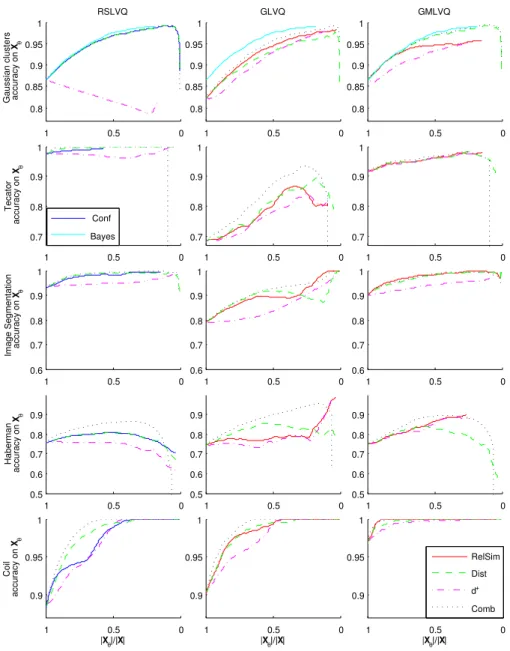
Figure 2 displays all results. For RSLVQ for Gaussian clusters, Conf, Dist and Comb provide nearly the same shape as the optimal reject option of the Bayes classifier. The same behavior occurs for RelSim, Dist and Comb with the
G(M)LVQ model. Onlyd+shows poor results not only for Gaussian clusters but
also for the other data sets. This can be an indicator that there are less outliers than ambiguous data points in the data. In nearly all models and for all data sets, Comb constitutes the best reject measure, but being based on two thresholds it is not efficient. RelSim and Dist provide comparable curves with less effort except for Tecator (GLVQ) and Haberman (RSLVQ, GLVQ). As a conclusion, we can see that RelSim in combination with GMLVQ offers an efficient certainty measure with a quality comparable to optimum reject strategies in almost all settings, but releasing the burden of an explicit probabilistic modeling for Conf or optimization of different objectives for Comb.
5
Conclusion
We have compared several efficient geometric reject measures for prototype-based approaches with statistical reject strategies on benchmark data sets. We
0 0.5 1 0.8 0.85 0.9 0.95 1
Gaussian clusters accuracy on Xθ RSLVQ 0 0.5 1 0.8 0.85 0.9 0.95 1 GLVQ 0 0.5 1 0.8 0.85 0.9 0.95 1 GMLVQ 0 0.5 1 0.7 0.8 0.9 1 Tecator accuracy on Xθ 0 0.5 1 0.7 0.8 0.9 1 0 0.5 1 0.7 0.8 0.9 1 0 0.5 1 0.6 0.7 0.8 0.9 1
Image Segmentation accuracy on Xθ 0 0.5 1 0.6 0.7 0.8 0.9 1 0 0.5 1 0.6 0.7 0.8 0.9 1 0 0.5 1 0.5 0.6 0.7 0.8 0.9 Haberman accuracy on Xθ 0 0.5 1 0.5 0.6 0.7 0.8 0.9 0 0.5 1 0.5 0.6 0.7 0.8 0.9 Conf Bayes 0 0.5 1 0.9 0.95 1 |Xθ|/|X| Coil accuracy on Xθ 0 0.5 1 0.9 0.95 1 |Xθ|/|X| 0 0.5 1 0.9 0.95 1 |Xθ|/|X| RelSim Dist d+ Comb
Fig. 2: Average results of mentioned rejection options when applying RSLVQ, GLVQ and GMLVQ models trained for different data sets. We display the
relative size of Xθ vs. the accuracy of the classifier on this set. The averaged
curve is plotted, where at least 80 % of the single runs deliver a value.
applied the reject options to different models: GLVQ as popular LVQ scheme based on a cost function, GMLVQ which uses a metric adaption, and RSLVQ
which provides a statistically motivated discriminative model. We showed that geometrically motivated measures (RelSim, Dist, Comb) can be used to im-prove the accuracy of a model and they lead to results comparable to optimum Bayes reject strategies (e. g. using GMLVQ and RelSim) but releasing the bur-den of explicit statistical modeling. This opens the way towards the design of efficient life-long model adaptation for popular prototype-based classifiers such as GMLVQ: the model complexity can easily be tailored online towards regions with a low certainty of the classification, e. g. introducing novel prototypes which are capable of representing novel aspects of the data.
References
[1] P. Schneider, M. Biehl, and B. Hammer. Adaptive Relevance Matrices in Learning Vector Quantization. Neural Computation, 21(12):3532–3561, 2009.
[2] S. Seo and K. Obermayer. Soft Learning Lector Quantization. Neural Computation, 15(7):1589–1604, Jul 2003.
[3] C. Campbell and Y. Ying.Learning with Support Vector Machines. Morgan and Claypool, 2011.
[4] I. W. Tsang, J. T. Kwok, and P.-M. Cheung. Core vector machines: Fast SVM training on very large data sets.Journal of Machine Learning Research, 6:363–392, 2005. [5] J. C. Platt. Probabilistic Outputs for Support Vector Machines and Comparisons to
Regularized Likelihood Methods. InAdv. in Large Margin Classifiers. MIT Press, 1999. [6] T.-F. Wu, C.-J. Lin, and R. C. Weng. Probability Estimates for Multi-class Classification by Pairwise Coupling.Journal of Machine Learning Research, 5:975–1005, August 2004. [7] G. Fumera and F. Roli. Support Vector Machines with Embedded Reject Option. In
Proceedings of the Int. Workshop on Pattern Recognition with Support Vector Machines (SVM2002), Niagara Falls, pages 68–82. Springer, 2002.
[8] R. Hu, S. J. Delany, and B. Mac Namee. Sampling with Confidence: Using k-NN Con-fidence Measures in Active Learning. In Proceedings of the UKDS Workshop at 8th International Conference on Case-based Reasoning, ICCBR’09, pages 181–192, 2009. [9] E. Ishidera, D. Nishiwaki, and A. Sato. A confidence value estimation method for
hand-written Kanji character recognition and its application to candidate reduction. Interna-tional Journal on Document Analysis and Recognition, 6(4):263–270, April 2004. [10] S. Kirstein, H. Wersing, H.-M. Gross, and E. K¨orner. A Life-Long Learning Vector
Quantization Approach for Interactive Learning of Multiple Categories.Neural Networks, 28:90–105, 2012.
[11] A. Sato and K. Yamada. Generalized Learning Vector Quantization. InAdvances in Neural Information Processing Systems, volume 7, pages 423–429, 1995.
[12] C. K. Chow. On Optimum Recognition Error and Reject Tradeoff. InIEEE Transactions in Information Theory, volume 16(1), pages 41–16, 1970.
[13] M. Biehl, K. Bunte, and P. Schneider. Analysis of flow cytometry data by matrix relevance learning vector quantization. PLoS ONE, 8(3):e59401, 2013.
[14] A. Vailaya and A. K. Jain. Reject Option for VQ-Based Bayesian Classification. In
International Conference on Pattern Recognition (ICPR), pages 2048–2051, 2000. [15] T. Martinetz and K. Schulten. Topology representing networks. Neural Networks, 7:507–
522, 1994.
[16] K. Bache and M. Lichman. UCI machine learning repository, 2013.
[17] S. A. Nene, S. K. Nayar, and H. Murase. Columbia Object Image Library (COIL-20).
Technical Report CUCS-005-96, February 1996.
[18] L. J. P. van der Maaten. Matlab Toolbox for Dimensionality Reduction, March 2013. http://homepage.tudelft.nl/19j49/Matlab Toolbox for Dimensionality Reduction.html. [19] H. H. Thodberg. Tecator data set, contained in StatLib Datasets Archive, 1995.