Peter Palmroos
Effect of unobserved defaults on
correlation between probability
of default and loss given default
on mortgage loans
Bank of Finland Research
Discussion Papers
Suomen Pankki Bank of Finland PO Box 160 FI-00101 HELSINKI Finland +358 10 8311
Bank of Finland Research
Discussion Papers
3
•
2009
Peter Palmroos*
Effects of unobserved defaults
on correlation between
probability of default and
loss given default
on mortgage loans
The views expressed in this paper are those of the author and do not necessarily reflect the views of the Bank of Finland. * E-mail: [email protected]
http://www.bof.fi ISBN 978-952-462-486-2 ISSN 0785-3572 (print) ISBN 978-952-462-487-9 ISSN 1456-6184 (online)
Effects of unobserved defaults on correlation between
probability of default and loss given default on
mortgage loans
Bank of Finland Research
Discussion Papers 3/2009
Peter Palmroos
Monetary Policy and Research Department
Abstract
This paper demonstrates how the observed correlation between probability of default and loss given default depends on the fact that defaults in which collateral provides 100% recovery are not observed. Creditors see only the defaults of mortgagors who suffer from a fall in collateral value to less than the remaining loan principal. Consequently, the default data available to creditors amounts to a mere truncated sample from the underlying population of defaults. Correlation estimates based on such truncated samples are biased and differ substantially from estimates derived from representative non-truncated samples. Moreover, the observed correlation between default probability and loss given default is sensitive to the truncation point, which may explain the differences in correlation estimates found in the literature. This may also explain why correlation estimates seem to be specific to cycle phase.
Keywords: credit risks, mortgage loans, truncated distributions, sample selection, log-normal distribution
Havaitsemattomien maksukyvyttömyystapausten
vaikutus asuntoluottojen tappiotodennäköisyyden ja
tappio-osuuden väliseen korrelaatioon
Suomen Pankin keskustelualoitteita 3/2009
Peter Palmroos
Rahapolitiikka- ja tutkimusosasto
Tiivistelmä
Tämän työn tarkoituksena on osoittaa, miten havaintojen perusteella estimoitu korrelaatio tappiotodennäköisyyden (probability of default, PD) ja tappio-odotuk-sen (loss-given-default, LGD) välillä riippuu siitä, etteivät kaikki maksukyvyt-tömyystapaukset (default) ole pankkien havaittavissa. Lainanantajat pystyvät var-muudella havaitsemaan vain ne maksukyvyttömyystapaukset, joissa vakuuden arvo ei enää kata jäljellä olevaa lainaa. Tapaukset, joissa vakuus kattaa koko jäl-jellä olevan lainapääoman ja kertyneet korot, eivät sen sijaan ole varmuudella havaittavissa, ja niitä on joka tapauksessa vaikea erottaa normaaleista asunnon-vaihtoon liittyvistä ennenaikaisista takaisinmaksuista. Näin ollen lainanantajien rekisteröimät maksukyvyttömyystapaukset ovat ainoastaan katkaistu otos kaikkien maksukyvyttömyystapahtumien joukosta. Korrelaatioestimaatit, jotka perustuvat tällaisiin katkaistuihin otoksiin ovat harhaisia ja eroavat huomattavastikin niistä estimaateista, jotka on laskettu katkaisemattomasta havaintojoukosta. Lisäksi havaitut korrelaatiot tappiotodennäköisyyden ja tappio-odotuksen välillä ovat herkkiä katkaisupisteen sijainnin suhteen. Toisistaan poikkeavat katkaisupisteet saattavat selittää eron julkaistujen tutkimusten korrelaatioestimaattien välillä. Jakauman katkaisu selittää myös, miksi joissain tutkimuksissa on havaittu korre-laation suhdanneriippuvaisuutta.
Avainsanat: luottoriski, asuntoluotot, katkaistu jakauma, kaksiulotteinen log-normaali jakauma
Contents
Abstract ... 3
Tiivistelmä (abstract in Finnish) ... 4
1 Introduction ... 7
2 Default in mortgage loan credit risk model ... 10
3 Derivation of conditional correlation between PD and LGD ... 11
3.1 Correlation of truncated bivariate distribution ... 14
3.2 Bivariate normal distribution ... 15
3.3 Bivariate log-normal distribution ... 16
3.4 Difference in correlation between subsamples and the case of sample selection ... 19
4 Some empirical results and implications ... 21
5 Conclusion ... 24
1 Introduction
The subprime crisis has underlined the role of mortgage loans as a potential source of credit risk and contagion. The crisis has also spotlighted the importance of correct risk-based pricing of mortgage loans. Due to the growing risks and the modeling of credit risk under the new Basel capital accord, mortgage loans have become an important topic of research.
One of the key issues in credit risk modeling is the correlation between probability of default (PD) and loss given default (LGD). In earlier studies a nonzero correlation has been found in corporate loan and bond data. For example, Frye (2000b), Altman et al (2002), and Das (2007) find support for the assumption of positive correlation between these risk components. Altman, Resti and Sironi (2002) also find that many recent studies present evidence of the same economic factors being behind both PD and LGD which would explain positive correlation.
The macroeconomic mechanism for the PD-LGD dependence of mortgage loans is very similar to that for corporate loans. Conditions that lead to an increase in corporate bankruptcies also raise the probability of unemployment; and the dependence between housing prices and collateral values for corporate loans is presumably very strong. One might well expect to see similar correlations and interdependence among mortgage credit risk components. Van Order (2007)finds evidence that the correlation effect exists within a group of mortgage loans, which supports this expectation.
Using an incorrect correlation estimate might cause serious errors in the risk and price calculations that are essential to mortgage lenders as well as to
financial supervisors. But these two are not the only possible victims of false estimates of such correlations. For whole markets, even bigger effects can come via mispricing and underestimation in connection with CDOs and mortgage backed securities. Incorrectly estimated correlation between PD and LGD can lead to underestimation of expected credit losses and undersized capital allocations. Such misspecification of credit risks could falsely lull banks and supervisors concerning the safety issue just when allocated capital is insufficient due to the low expected PD-LGD correlation. Frye (2000a) highlights the importance of correlation and reminds us that a severe downturn might bring a double hit on banks if macro factors simultaneously increase both PD and LGD and cause larger credit losses to banks than are predicted by the models. The double hit is possible when both the number of defaults and the collateral values are dependent on the same macroeconomic factors.
The empirical literature includes a wide range of estimated correlation between PD and LGD. Using data on corporate loans with different breakdowns, researchers have found correlations from zero to as high as 0.8.1
Most of the reported estimates are near the lower end of this range. For example, for data from Altman and Kishore (1996), the correlation is 0.3. This evidence should not, however, be seen to indicate that assuming independence between PD and LGD would be realistic. The independence assumption has
1Carey and Gordy (2001) report correlations close to zero and Frye (2000b) reports a
also been rejected, for example, in papers by Chabaane et al (2004) and Schuermann (2004). This is also in line with Altman et al (2001), who argue that a model in which both PD and LGD behave stochastically and are partially dependent, seems to be the most realistic. Altman, Resti and Sironi also present a list of other papers supporting this argument.
At least a couple of explanations for the low correlation estimates can be found in the literature. Schuermann (2004) presents evidence that the correlation has been masked by the weighting of the data. Hu and Perraudin (2002) have another explanation: the reported correlation might be lower than the true correlation because of the industry breakdown that was used. Both explanations could contain seeds of truth, but neither tells the whole story nor is applicable to all datasets.
Estimated correlations have also varied across data subsets. A common case in the literature is where the data are divided into subsets using a variable that describes the different phases of the business cycle. This resulted in unequal estimates of correlations for the different subsets. For example, Hu and Perraudin (2002) estimate the correlation to be 0.2 in normal situations and 0.3 inside the tail subsample.2 Das (2007) report that in the set of observations for years when default rates were high and recovery rates low, the correlation became larger in absolute value. Similarfindings are reported in the survey of Altman et al (2002), which compares the results of Carey and Gordy (2001) and Frye (2000b). Using the whole sample, Carey and Gordy obtain a correlation very close to zero, in contrast to thefindings of Frye. After dividing the sample into different time periods, the subsample correlations are closer to the higher correlation reported by Frye. Although there is evidence to suggest that the relationship between default rates and LGD is influenced by the current phase of the business cycle, as in Altman et al (2002), we still lack a convincing explanation of the dependency on cycle phase.
This paper presents a possible reason for these lower-than-expected observed correlations and for the cycle-phase-specific correlation estimates. Findings presented in this paper help explain why one should be suspicious of small correlations between PD and LGD presented in the other papers. A critical attitude toward the estimates and estimation methods presented in the literature should obtain, especially when these correlation estimates are to be used in credit risk modeling and eg in identifying downturns or stressed LGD. In estimating the correlation between PD and LGD one typically uses the observed number of defaults and realized LGDs. However creditors’ ability to observe defaults is limited. If the value of collateral covers the remaining principal and accrued interest on the loan, the creditor might be unable to observe the default, because the debtor is able to pay the remaining principal after realizing the collateral. The situation can be considered a default because the debtor is unable to pay amortization and interest without realizing the collateral. If the realization of collateral occurs without delay, the creditor cannot distinguish a default without loss from the normal house transfer process. If there is some delay in the realization, a creditor might be able
2Hu and Perraudin (2002) found a negative correlation between PD and recovery rate
to observe a lossless default. But observations of defaults without loss are of limited usefulness because creditors are unable to determine the number of these from the total number of lossless defaults.
Creditors can certainly observe defaults where the value of collateral is less than the remaining principal. These observed defaults, whose LGD is strictly between zero and one, make up a truncated sample from the set of all defaults. If a borrower has other collateral in addition to the house or there is some kind of safety net for defaulting borrowers, even these defaults may be difficult to observe. For simplicity, this paper assumes that the house is the only collateral and that there is no safety net.
The correlation from a truncated sample is, except for some extreme cases, lower than that from the unrestricted data set, and the difference may be huge. Because of the possibility of a huge difference, it is important to ensure that the truncation of default events is accounted for in the credit risk calculations. The low correlation estimates found in the literature could result from the omission of the effects of truncating and including only observed defaults in the correlation calculations.
The value of collateral is dependent on the current phase of the business cycle. In a boom phase, the value of collateral increases, and hence the coverage of the collateral increases and the LGD decreases. In times of recession, these changes are reversed. The effect of the dependence between cycle phase and LGD strengthens if the number of defaults-LGD data is divided into two subsets based on cycle phase and the correlation estimated separately for the subsets. Because of the dependence between cycle phase and LGD, data splitting can be considered sample selection. Such sample selection leads to doubly truncated data where correlations of non-recession events are lower than correlations of recession events and the correlation estimates for both groups are substantially lower than the correlation found in the dataset as in total between defaults and LGDs.
Using these observed correlations instead of the correlation between unconditional variables in credit risk modeling and in risk-based capital allocation models leads to underestimation of both expected losses and capital requirements. This can be readily seen when banks try to calculate downturn LGD estimates where downturn LGD is a cycle-phase-dependent LGD estimate. The use of parameters estimated from such a misconstructed distribution in this type of calculation can lead to totally misleading point estimates and confidence intervals.
The empirical data from Finland, Germany, UK, USA, and Spain supported the assumption of negative correlation between probability of default and value of collaterals and shed light on the level of this unobserved correlation. Finnish data are used for estimating observable correlations, which are calculated using several loan-to-values truncation points.
This paper is organized as follows. Section 2 describes the theory and the default framework used in this paper. Section 3 presents the concept of conditional probability of default and conditional loss given default, as well as the closed solutions to correlations of truncated bivariate normal and log-normal distributions. Section 4 discusses the empirical implications, and some concluding remarks are given in section 5.
2 Default in mortgage loan credit risk model
Papers on credit risk of mortgages have already adopted well known theories of corporate loans, such as the various extensions of the Merton (1974) structured model and the hazard rate models. The dominance of corporate loan credit risks in modeling can be seen from the fact that only a few mortgage-specific credit risk theories have been presented in the literature. This has also been observed by Whitley et al (2004), who find that most papers on mortgages focus on describing empirical findings rather than establishing theories for credit risks. Comprehensive surveys of credit risk theories applied to corporate loans include Allen and Saunders (2003) and Altman et al (2001).
One of the differences between corporate and private loans is in the meaning of default. Neither in practice nor in the literature has there been a complete description of a default on a mortgage. The papers on mortgages have either relied on default descriptions presented in the literature on corporate-loan credit risk or they have formulated descriptions specific to the particular paper. Not only is the description of a mortgage loan default more difficult than that for a corporate loan but so too are the observation and identification of mortgage defaults more problematic in practice.
One way to explain the concept of default is to assume that behind a default is some trigger event. Depending on the economic and juridical environment, the significance of these triggers can vary. Some of them may be independent of the borrower’s debt. One example of an independent trigger event is to become unemployed. In contrast, some triggers are dependent on the features of the loan. For example, a decrease in the coverage of collateral can lead to default in certain legal environments. Some of the possible triggers have been presented and categorized in the paper by Cairns and Pryce (2005).
The economic and juridical environment has a pronounced effect on which triggers can lead to default. One way to categorize mortgage credit risk theories is by the manner in which rational debtors react to certain possible triggers. Whitley et al (2004) separate these theories into two groups: equity theories and ability-to-pay -theories.
In the equity-theories framework, the rational debtor, with a slight simplification, defaults as soon as the value of collateral sinks below the remaining mortgage loan principal. Such behavior is rational if the local law allows personal bankruptcy and if the mortgage loan can be cleared by assigning the collateral to the creditor. An example of such a theory is presented by Kau et al (1992).
In many countries the law does not allow personal bankruptcy, so that the debtor is liable for the remaining loan after realization of the collateral. In such an environment, voluntary default is irrational because the difference between the loan principal and the value of the collateral remains as customer’s debt after the default. Whitley et al (2004) refer to these approaches as ’ability-to-pay’ theories. These assume that a default is an undesired result of debtor insolvency and never a result of rational choice.
The model presented in this paper can fit into either of these approaches without substantial modification. In the equity-theory approach there should be an additional trigger describing the borrower’s rational choice to default.
Such a rationality trigger is positively dependent on the current loan-to-value ratio (LtV). One model in which the probability of default is dependent on the collateral value is that by Dimou et al (2005).
In neither of the two frameworks is the creditor is able to observe the borrower’s default if the collateral value exceeds the remaining principal plus accrued interest. This is a consequence of the assumption of a rational debtor. Should a rational debtor face any of the default-triggering events when the collateral value covers the remaining principal, he will realize the collateral and repay the loan.
In this paper a default event is independent of whether or not it is observable to creditor. To separate observable defaults from those that are not dependent on the creditor’s ability to observe them, the later are referred to as unconditional defaults and their probabilities are denoted as PDU.
The concept of unconditional default makes it possible that the LGD is negative. In such case the value of the collateral exceeds the value of remaining principal. Of course, it is only the debtor who benefits here; for the creditor the LGD is equal to zero.
For defaults that creditors can observe, LGD is between zero and one. In this paper such defaults will be called conditional defaults and their probabilities are denoted PDC. The connection between unconditional and
conditional default can be written as
P DC =P DU|LGD>0 (2.1)
The observed defaults do not comprise a random sample from all defaults, because all observations where the default occurs when the collateral value exceeds the remaining principal are omitted, and so the ability to observe default is dependent on the value of the collateral. This is in line with the papers of Ambrose et al (1997), Chabaane et al (2004), and Dimou et al (2005).
3 Derivation of conditional correlation between PD
and LGD
The model used in this paper has elements of both hazard rate models and structural models based on the paper of Merton (1974). The connection with the hazard rate model is clear from the assumption that the default-trigger is exogenous. In this paper, we assume that only one trigger event can cause the default and that the trigger event is independent of the collateral value. These assumptions simplify the default modeling, since possible interdependences among triggers are omitted. The assumptions also mean that the default process coincides with the trigger event process.
The probability of a single default depends on the probability of a trigger event. In this model, default D and trigger T are binary variables equal to zero for events without default and unity for default events. The probability that default occurs (that D = 1) is equal to the probability that one or more
triggers T take the value one . The number of possible triggers is m. The probability of a trigger taking the value one, like the probability of default, is dependent on the macroeconomic variables included in vectors C and G1.
Under the assumption that there is no dependence between single defaults, ie that one borrower’s default does not cause another’s default, we can calculate PDU. Researchers such as Allen and Sounders (2003), Gross and Souleles
(2002), and Erlenmaier and Gersbach (2001) have found evidence supporting the assumption of PD being dependent on macroeconomic variables. This dependence can be seen as higher numbers of defaults in economic downturns.
P DU =P(D = 1|C, G1) =P [(T1 = 1∨T2 = 1∨. . .∨Tm = 1)|C, G1] (3.1)
The value of collateral, as well as the value of PD, is dependent on several macroeconomic variables. At least Allen and Saunders (2003), Frye (2000b), Frye (2003), and Schuermann (2004) have found evidence of higher LGD in recessions than during expansions. Frye (2000a) states that higher LGDs in recessions are a consequence of lower collateral values. The assumptions of this paper are in line with these findings. Due to the dependence between LGD and macroeconomic variables, both PD and LGD seem to move simultaneously, and this also causes the correlation between these components.
The loan-to-value (LtV) is the ratio of remaining principal to collateral value. The amortization period is assumed here to coincide with the observation period, so that the remaining principal can be taken as a constraint. The LtV follows the known process g, which is dependent on the values of the vectors C and G2, which include macroeconomic variables,
and theλ vector of loan-specific parameters. The function g should take only positive values:
LtVU =g(C, G2, λ) (3.2)
Both PD and LtV are dependent on the common explanatory variables C. As long as C is not a zero length vector, there is a relation between PDU and
LtVU.
Hence the model has some similarities with structural models. In the basic case of structural models, default occurs when asset value falls below a certain threshold, ie total liabilities. This kind of default trigger works only partly in equity-theories. In ability-to-pay contexts, this type of approach is suitable for the LGD but not the PD.
In our model the process of collateral value replaces the process of asset value used in the structural models. The threshold value can be replaced by the remaining mortgage loan principal. If both of these values are divided by the remaining principal, the collateral process can be replaced by the LtV−1
process and the threshold value is equal to 1.
When creditors estimate the LGD, they should include not only the remaining principal and accrued interest but also other default-related costs, such as recovery commissions. LGD is not unambiguous even after of all the included costs are determined, as long as the timetable for recovery is not determined. In this paper LGD is divided into long and short term LGD.
The difference between short and long term LGD is important when the ability to observe default depends on the ratio between remaining principal and collateral value. Short term LGD is the ratio of remaining principal to collateral value at the moment of default. The definition of long term LGD is closer to the definition used in Basel II. In environments where personal bankruptcy is not possible and where the remaining principal after realization of collateral remains as a liability to the debtor, the long term LGD will be close to zero. When a private person’s bankruptcy ‘clears the table’ from the debtors’ perspective and leaves the rest of the loan as a loss to creditor, the long term LGD will be much higher. Assuming the ability-to-pay context and a rational creditor, the short term LGD is always higher than the long term LGD.
In this paper the ability to observe default is dependent on the ratio of remaining principal to collateral value at the moment of default. For this reason, the short term LGD is a more reasonable value than the long term LGD for the purpose of modeling risk. Later in this paper the LGD is assumed to coincide with short term LGD.
LtV can be transformed into LGDU where the subscript U means
unconditional
LGDU = 1−LtVU−1 (3.3)
The value of LtVU determines whether a default can be observed. Defaults
where LGDU ≤ 0 (LtVU ≤ 1) are unobservable to the creditor.
The findings of this paper do not depend on the functional forms of PD and LtV, and so we simplify the analysis by assuming that the PD and LtV values come from known distributionsΦandΘwith parameter vectorsα1 and
α2. The assumption of a single trigger behind unconditional PD implies that Φis actually the distribution of the trigger event
P DU ∼Φ(α1) (3.4)
When there is only one type of collateral, ie the house, Θ is the distribution of collateral values.
LtVU−1 ∼Θ(α2) (3.5)
Because the processes of both PD and LGD are assumed to be dependent on the same variables, this relation can be observed as a correlation between PD and LGD
Cor(P DU, LtVU−1) =ρ P D,LtV
U (3.6)
Replacing the variable LtV by the variable LGD, yields the correlation
The correlation between PDU and LGDU can be written as Cor(P DU, LGDU) =ρU (3.8) Thus ρU =−ρ P D,LtV U (3.9)
To move to the conditional (observable) variables PDC and LGDC, we write
P DC =P DU|LtV−1
U >1 =P DU|LGDU>0 (3.10)
LGDC =LGDU|LtVU−1>1 =LGDU|LGDU>0 (3.11)
And the correlation between these conditional variables is
Cor(P DC, LGDC) =ρC (3.12)
When the variables PDU and LGDU generate a bivariate distribution with
correlation ρU , the conditional variables PDC and LGDC generate a similar
distribution, except that it is truncated at the point where LGDU = 0, so that
only events on the right side of the truncation point (0 < LGDU ≤ 1) are
included.
It should be noted that in most of the cases the observed correlation ρC
is not equal to the unconditional correlation ρU. The key issue concerns the
difference between unconditional and observed conditional correlation.
The methodology used in this paper can be applied (after small modifications) also in the case where all defaults can be observed but LGDs with zero or negative values are observed as zero values. In the latter case, we end up with a bivariate censored distribution instead of the bivariate truncated distribution.
3.1
Correlation of truncated bivariate distribution
It is possible (albeit not likely) that correlations between PDU and LGDU
change over time and that the dependence between credit risk factors differs for different time spans. But even with the assumption of constant unconditional correlation between these factors it is possible to observe different correlations. In this paper the unconditional correlation between the value of collateral and the probability of default is assumed to remain stable.
Since the distributions of defaults and collateral values are known, the truncated correlation can be estimated via simulation. But with certain bivariate truncated distributions one can use closed solutions. This paper utilizes the closed solutions of the truncated bivariate normal distribution and log-normal distributions. Normal distributions are more widely used and better known, whereas log-normal distributions have many more favorable properties. Use of the log-normal distribution also gets support from both theory and empirical findings.
3.2
Bivariate normal distribution
The closed solution to the observable correlation ρC between two normally
distributed variables with only one variable truncated and unconditional correlation ρU, can be found in the econometric and statistics literature. The
derivation of the formula is in Kotz et al (2000) and the solved correlation equation is presented for example in Cambell et al (2008)
ρC = r ρU ρ2 U+ (1−ρ2U) σ2 LGD σ2 LGD|T runcated (3.13)
The variance of the truncated variable LGD can be solved using the formula given in Johnson and Kotz (1970). The slightly modified equation for a single truncation point is presented in the book by Greene (2003). Variance of the truncated variable can be calculated as
σ2LGD|T runcated =σ2LGD(1−δ(α)) (3.14)
where the normalized truncation pointα is
α= (a−μLGD σLGD ) (3.15) and λ(α) = ( −φ(α)
Φ(α) right truncated f rom α (x > a omitted) φ(α)
1−Φ(α) lef t truncated f rom α (x < a omitted)
(3.16)
and
δ(α) =λ(α)(λ(α)−α) (3.17)
It can be seen that the absolute value of the observed correlation is less than or equal to the unconditional correlation. The points where both observed and unrestricted correlations are equal are where there is no correlation between the variables (ρObserved = ρU nrest = 0) and where the variables are perfectly
positively or negatively correlated (ρObserved =ρU nrest =±1).
The correlation formula also applies with a double truncated variable. The variance formula for a double truncated variable is found for example in Kotz (1970).
3.3
Bivariate log-normal distribution
A theoretically more viable framework than that of normally distributed variables is provided by the bivariate log-normal distribution, which forces values of both variables to be positive. The closed solution for this kind of setup is more complex than the solution for the truncated bivariate normal distribution. The solution presented here was used to enable the double truncation that will be used later in this paper. Values for the single truncation cases can be obtained by setting the unrestrictive limit at positive or negative infinity. Derivation of truncated bivarite log-normal formulas can be found in Vilmunen (2008).
In the following formulas, the probability of default follows a log-normal distribution LN(μP D, σP D) and loss given default follows LN(μLGD, σLGD).
Thus the mean (M) and variance (Σ2) of PD are
MP D =eμP D+
σ2P D
2 (3.18)
Σ2P D =e2μP D+σ2P D(eσ2P D −1) (3.19)
The mean and variance of LGD can be calculated with the same formulas. If PD ∼LN(μP D, σP D), then ln(PD) ∼N(μP D, σP D), and this also holds
for LGD. For calculating the truncated correlation, one needs the correlation between ln(PD) and ln(LGD). This correlation is denoted ρP D,LGD. Thus,
when the correlation between PD and LGD is ρU, the correlation of ln(PD)
and ln(LGD) can be calculated using the formula
ρP D,LGD = ln(ρU p eσ2 P D −1 p eσ2 LGD −1 + 1) σP DσLGD (3.20)
The previous formula and the requirement that the value of ρU and ρP D,LGD
must be contained in [-1, 1] imply that the smallest possible ρU can be
calculated by using ρP D,LGD and solving the equation for ρU.
The correlation formula for the truncated bivariate log-normal distribution follows the conventional correlation formula.
ρC = q σLGD,P D|T runcated σ2 LGD|T runcated q σ2 P D|(LGD|T runcated) (3.21)
The restricted variances and covariance needed for calculating the correlation can be obtained using the following formulas. A complementary way to solve for the variance of the truncated variable is to use the relation between non-truncated and truncated moments. This type of solution is presented in Johnson and Kotz (1970).
The variance of truncated log-normally distributed variable LGD is
σ2 LGD|T runcated=e 2μLGD+σ2LGD n eσ2 LGD h Φ(U3)−Φ(L3) Φ(U1)−Φ(L1) i −hΦ(U2)−Φ(L2) Φ(U1)−Φ(L1) i2¾ (3.22)
where the upper (U) and the lower (L) limit parameters with truncation points aU > aL are U1 = ln(aU)−μLGD σLGD L1 = ln(aLσ)−μLGD LGD (3.23) U2 = ln(aU)−(μLGD−σ2LGD) σLGD L2 = ln(aL)−(μLGD−σ2LGD) σLGD (3.24) U3 = ln(aU)−(μLGD−2σ2LGD) σLGD L3 = ln(aL)−(μLGD−2σ2LGD) σLGD (3.25)
The variance of the other log-normal variable PD conditional on the truncation of variable LGD is σ2P D|(LGD|T runcated) =e2μP D+σ2P D n eσ2P D h Φ(U6)−Φ(L6) Φ(U1)−Φ(L1) i −hΦ(U5)−Φ(L5) Φ(U1)−Φ(L1) i2¾ (3.26)
where the upper (U) and the lower (L) limit parameters for truncation point aU > aL are U5 = ln(aU)−(μLGD+σLGDσP DρP D,LGD) σLGD L5 = ln(aL)−(μLGD+σLGDσP DρP D,LGD) σLGD (3.27) U6 = ln(aU)−(μLGD+2σLGDσP DρP D,LGD) σLGD L6 = ln(aL)−(μLGD+2σLGDσP DρP D,LGD) σLGD (3.28)
The last required value, the covariance between variables LGD and PD after truncation of LGD, is σLGD,P D|T runcated=eμLGD+μP D+ 1 2(σ 2 LGD+σ 2 P D) ×neρP D,LGDσLGDσP D hΦ(U 4)−Φ(L4) Φ(U1)−Φ(L1) i −hΦ(U2)−Φ(L2) Φ(U1)−Φ(L1) i hΦ(U 5)−Φ(L5) Φ(U1)−Φ(L1) io (3.29)
and the upper (U) and the lower (L) limit parameters and truncation point aU
>aL are U4 = ln(aU)−(μLGD−σ2LGD+σLGDσP DρP D,LGD) σLGD L4 = ln(aL)−(μLGD−σ2LGD+σLGDσP DρP D,LGD) σLGD (3.30)
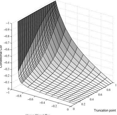
An example of dependence between ρU and ρC with a varying truncation
point is presented infigure 1. With the log-normal distribution, the truncated correlation can be lower or higher than the unconditional correlation. A higher truncated correlation is possible only when ρU is very close to its lower limit
(here, -0.968). When the parameter values are close to those used in figure 1, the truncated correlation is lower than ρU for all correlations found in the
economic data samples. If the highly improbable extremely high negative correlations are eliminated, then the larger the gap between collateral value and the remaining principal at the start of the observation period, the lower the correlation between observed defaults and positive LGDs
Thisfinding has at least two implications. First, the correlation in a sample of observed defaults should be lower if the sample is taken from a market where LtV is systemically lower than it would be if the sample were taken from a market with higher LtVs. It should be noted that changes in loan markets, ie tightening competition between creditors, might also change the LtV for new loans. This is one possible explanation for the differences in correlation estimates across the various papers that use samples from similar environments.
The other implication is that in times of booming markets the ratio of remaining principal to collateral value decreases and in recession the ratio increases. Thus, during different cycle phases, the older loans could affect the number of observed defaults, which could widen the difference between correlations, at least in the sample selection case.
−1 −0.8 −0.6 −0.4 −0.2 0 0 0.2 0.4 0.6 0.8 1 −1 −0.9 −0.8 −0.7 −0.6 −0.5 −0.4 −0.3 −0.2 −0.1 0 Truncation point Unconditional Cor Conditional Cor
Figure 1. Dependence between ρU and ρC.Dependence between ρU and
truncated variables ρC when MP D = 0.120, ΣP D = 0.035, MLGD = 1.045, ΣLGD = 0.08. Minimum value of ρU is -0.968, and LtV is between 0.1 and 1.
3.4
Difference in correlation between subsamples and the case
of sample selection
Besides the low correlations, the earlier papers have found that the correlation can vary depending on the phase of the business cycle. One possible reason for this is the ignored sample selection.
Sample selection could be a consequence of using a macroeconomic variable as an instrument for selecting events to include in different subsamples in cases where the variable is also a factor in the changes in LGD. Thus dividing the sample of observed defaults using a macro factor such as GDP growth as an instrument cause an extra truncation of the sample. This extra truncation divides the former single truncated sample into the single truncated severe downturn subsample and a double truncated subsample including non-recession observations.
Such sample selection might lower the observed correlation of a double truncated subsample nearly to zero. The correlation of a double truncated subsample is always smaller than that of a single truncated sample. The smaller the fraction of observations in the middle range, the lower the correlation. This can be seen from figure 2. Note the very large, almost
flat area, where the truncated correlation is close to zero. Also the correlation for tail observations, shown infigure 3, is smaller than the correlation for the original single truncated sample. The larger the fraction of observations in the downturn tail, the closer will be the correlation of these tail observations to the original single truncated PD-LGD correlation.
−1 −0.8 −0.6 −0.4 −0.2 0 0 0.2 0.4 0.6 0.8 1 −0.45 −0.4 −0.35 −0.3 −0.25 −0.2 −0.15 −0.1 −0.05 0 Truncation point Unconditional Cor Conditional Cor
Figure 2. Dependence betweenρU andρC of double truncated subsample.
Dependence between double truncated subsample ρC and ρU with MP D =
0.120, ΣP D = 0.035, MLGD = 1.045, ΣLGD = 0.08. Minimum value of ρU
is -0.968, and LtV is between 0.1 and 1. Z-axis is reversed, to facilitate interpretation.
−1 −0.8 −0.6 −0.4 −0.2 0 0 0.2 0.4 0.6 0.8 1 −0.7 −0.6 −0.5 −0.4 −0.3 −0.2 −0.1 0
Share of mid part Unconditional Cor
Conditional Cor
Figure 3. Dependence betweenρU andρC of tail observations. Dependence between recession observations (single truncated left tail) ρC and ρU with
MP D= 0.120, ΣP D = 0.035, MLGD = 1.045, ΣLGD = 0.08. Minimum value
of ρU is -0.968, and LtV is between 0.1 and 1. Z-axis is been reversed, to facilitate interpretation.
4 Some empirical results and implications
The Finnish empirical data illustrate how wide the gap may be between unconditional and observed correlations and how large the effect of sample selection on observed correlations may be.
From the creditor’s viewpoint, default means the customer’s insolvency or falling into arrears in a situation where the value of collateral is insufficient to cover the remaining loan. For credit risk research, as already has been established, this view is much too narrow, and it gives a distorted view of the default frequency of private persons and of the distribution of defaults in the whole population. Observing a private person’s default is not as unequivocal as is a default for a corporation. The accuracy of the estimated probability of default and the significance of the estimate for mortgage credit risk modeling are however dependent on successful observation of private persons’ defaults.
To get a broader and a more economically oriented view of a borrower’s default, this paper omits the default concepts used by banks and other creditors. Instead, a private person’s default is interpreted as a situation following a trigger event when the borrower is no longer able to pay amortizations and interest and collateral realization is the only possibility.
One commonly used trigger is unemployment. Because the possibility of becoming unemployed is independent of whether one has a mortgage loan, we can consider the probability of the borrower becoming unemployed as equal to the probability of a randomly chosen employed person becoming unemployed. In Finland, a house or shares in a housing company are the most commonly used types of collateral for mortgage loans. For this reason, the housing price index suffices as an indicator of overall developments in collateral values and changes in LtV. In this paper, the percentage changes in the Finnish housing price index (HPI) are used to estimate developments in collateral values. The time series of the housing price index can be found from the website of Statistics Finland (www.tilastokeskus.fi).
To estimate the default probability for a mortgagor, we need the probability of an appropriate trigger event. In this paper, we use the probability that an employee will become unemployed during a single observation period. The probability of default is calculated by dividing the number of persons unemployed at the end of the observation year whose unemployment bout has lasted less than a full year by the number of persons employed at the start of the period.
The idea behind this measure of PD is in the assumptions that only employed persons can obtain mortgage loans and that the probability of becoming unemployed does not depend on whether the employee has a mortgage loan. The time series used in the PD calculation can be found from the website of the Finnish Ministry of Employment and the Economy (www.tem.fi).
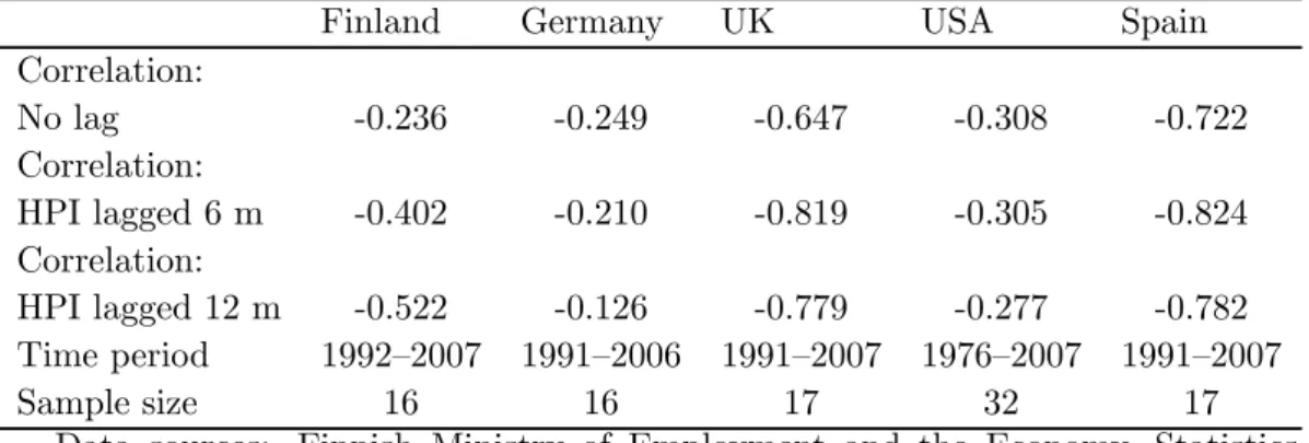
Correlation estimates using data from Finland, Germany, UK, USA, and Spain supported the assumption of negative dependence between PD and value of collateral. These estimates are presented in table 1. The correlation between collateral values and probability of default is calculated using three different lags for the housing price index (0, 6, and 12 months) relative to the observation period for unemployment. The motivation for the lags comes from the term of notice for layoffand the delay between layoffand registration as an unemployed job-seeker. As can be seen from the table, the correlation seems to vary remarkably depending from the lag structure. The US correlations are estimated using the number of newly unemployed whose unemployment period has been shorter than 27 weeks. For this reason, US estimates are not comparable with the others, but do support the assumption of this paper.
Table 1. Estimated correlation between PD and collateral value in Finland, Germany, UK, USA, and Spain
Finland Germany UK USA Spain
Correlation: No lag -0.236 -0.249 -0.647 -0.308 -0.722 Correlation: HPI lagged 6 m -0.402 -0.210 -0.819 -0.305 -0.824 Correlation: HPI lagged 12 m -0.522 -0.126 -0.779 -0.277 -0.782 Time period 1992—2007 1991—2006 1991—2007 1976—2007 1991—2007 Sample size 16 16 17 32 17
Data sources: Finnish Ministry of Employment and the Economy, Statistics Finland, Eurostat, Bundesarchitektenkammer e. V. (Germany), OFHEO (US), Bureau of Labor Statistics (US), Ministerio de vivienda (Spain), Office of Deputy Prime Minister (UK), and www.communities.gov.uk (UK).
When the unconditional correlation between PD and LGD is known, the conditional correlation can be estimated for both the single truncation and sample selection cases.
In the single truncation case, the importance of loan-to-value for the observed correlation can be seen from table 2. The table shows that both the loan-to-value ratio and the unconditional correlation should be relatively high before the absolute value of conditional correlation is high enough to be observed. These low correlations estimates, relative to the unobservable ones, are in line with figures reported by Hu and Perraudin (2002) and Carey and Gordy (2001), which are presented in the introduction.
Table 2. Estimates of observable correlationsρC of Finnish data with single truncation at different loan-to-value points and with three unconditional correlations from table 1.
LtV ρU =-0.236 ρU =-0.402 ρU =-0.522 1.0 -0.127 -0.239 -0.341 0.9 -0.086 -0.169 -0.252 0.8 -0.060 -0.121 -0.184 0.7 -0.043 -0.088 -0.136 0.6 -0.032 -0.067 -0.103 0.5 -0.025 -0.051 -0.079
In the sample selection case, the observed correlations for the tail and middle subsets depend on the truncation point dividing the data. In tables 3 and 4, the location of the truncation point was determined using the portion of observations to be included in the tail subset. In table 3 the loan-to-value at the start of the period was set at 0.7 and in table 4 all loans were assumed to be granted at 100% collateral value of, ie LtV was set at one.
Table 2 illustrates the fact that the estimated correlation is dependent on the location of truncation points. If for example the truncation point shifts due
to changes in banks’ lending (LtV) policies, the estimated correlations before and after the policy change will be different.
The effect of changing truncation points is even stronger in the case of sample selection, where the differences in cycle phase are used. This leads to the situation where, depending on the size of the double truncated area, the correlation estimate can be anything between zero and the correlation estimate of the single truncated data.
Tables 3 and 4 present results that are similar to those for example of Hu and Perraudin (2002), where the observed correlation for recession phases seems to be higher than the estimated correlation for normal conditions. It should be noted that the unconditional correlation remains constant even when the conditional observed correlations vary according to cycle phase.
Table 3. Observable correlations ρC of Finnish data with double truncation with loan-to-value equal to 0.7, number of double truncated mid-range observations in row headers and with three unconditional correlations from table 1.
Share of ρU= -0.236 ρU= -0.402 ρU= -0.522 Mid-range Left Tail Mid-range Left Tail Mid-range Left Tail Mid-range Observations 10 % -0.043 -0.001 -0.088 -0.003 -0.136 -0.004 20 % -0.043 -0.003 -0.088 -0.006 -0.135 -0.009 50 % -0.042 -0.009 -0.086 -0.018 -0.132 -0.028 80 % -0.041 -0.019 -0.084 -0.040 -0.127 -0.062 90 % -0.041 -0.026 -0.082 -0.053 -0.124 -0.082
Table 4. Estimates of observable correlationsρC of Finnish data with
double truncation withloan-to-value equal to 1.0, number of double truncated mid-rangeobservations in row headers and with three correlations from table 1.
Share of ρU= -0.236 ρU= -0.402 ρU= -0.522 Mid-range Left Tail Mid-range Left Tail Mid-range Left Tail Mid-range Observations 10 % -0.123 -0.006 -0.233 -0.012 -0.332 -0.019 20 % -0.120 -0.013 -0.226 -0.025 -0.323 -0.038 50 % -0.109 -0.036 -0.205 -0.070 -0.292 -0.104 80 % -0.094 -0.069 -0.176 -0.133 -0.251 -0.195 90 % -0.086 -0.087 -0.161 -0.167 -0.230 -0.242
5 Conclusion
Although this paper focuses on mortgage loans, the basic idea applies to other types of loans as well. The effect of truncation on pricing and risks should be studied at least with mortgage-linked products such as CDO and MBS. For these products, the effect of using only conditional correlation leads to large differences in estimated risks and thus to large differences in risk-adjusted prices.
Credit risk has been divided here into the same risk components used in the Basel capital requirement calculations and presented in the new Basel capital accord. The model presented here focuses on PD and LGD and the correlation between them. Due to assumption of homogeneous position, the effects of changes in exposure at default (EAD) were omitted. In reality, the phase of the business cycle could affect EAD, via changes in new loan principals, as well as in parameters such as LtV. These effects could be key to understanding differences in the credit risks of dynamic mortgage portfolios at different times and different phases of the business cycle.
As for future research, one might want to assume heterogeneous (rather than homogeneous) loan portfolios. Such a model can provide more information on the possible effects of a pick-up in the economy and mortgage lending on credit losses and on the effects of these on the observed correlations. The assumption of heterogeneous position structure would bring this credit risk model even closer to reality and so is worthy of further study.
References
Allen, L — Saunders, A (2003) Survey of cyclical effects in credit risk measurement models.BIS Working Papers (126).
Altman, E — Kishore, V (1996)Almost everything you wanted to know about recoveries on defaulted bonds. Financial Analyst Journal, 57—64. Altman, E — Resti, A — Sironi, A (2001)Analyzing and explaining default recovery rates.A Report Submitted to The International Swaps Derivatives Association.
Altman, E — Resti, A — Sironi, A (2002) The link between default and recovery rates: effects on the procyclicality of regulatory capital ratios. BIS Working Papers (113).
Ambrose, B — Buttimer, R — Capone, C (1997) Pricing mortgage default and foreclosure delay.Journal of Money 29 (3), 314—325.
Cairns, H — Pryce, G (2005) An analysis of mortgage arrears using the british household panel survey.University of Glasgow Working Paper. Campbell, R — Forbes, C — Koedijk, K — Kofman, P (2008) Increasing correlations or just fat tails? Journal of Empirical Finance 15 (Issue 2), 287—309.
Carey, M — Gordy, M (2001) Systematic risk in recoveries on defaulted debt.Unpublished Working Paper Presented a the 2001 Financial Management Association Meeting, Toronto.
Chabaane, A — Laurent, J-P — Salomon, J (2004) Double impact: Credit risk assessent and collateral value.www.defaultrisk.com.
Das, S (2007) Basel II: Correlation related issues. Journal of Financial Services Research 32 (1—2), 17—38.
Dimou, P — Lawrence, C — Milne, A (2005) Skewness of returns, capital adequacy, and mortgage lending. Journal of Financial Services Research 28 (1—3), 135—161.
Erlenmaier, U — Gersbach, H (2001) Default probabilities and default correlations.Working Paper Series.
Frye, J (2000a)Collateral damage. Risk 13 (4). Frye, J (2000b)Depressing recoveries. Risk, 106—111. Frye, J (2003)A false sense of security. Risk, 63—67.
Greene, W (2003)Econometric Analysis, fifth edition.Pearson Education Inc., New Jersey.
Gross, D — Souleles, N (2002) An empirical analysis of personal bankruptcy and delinquency. The Review of Financial Studies 15 (1) 319—347.
Hu, Y-T — Perraudin, W (2002) The dependence of recovery rates and defaults.CEPR Working Paper.
Johnson, N — Kotz, S (1970) Distributions in Statistics: Continuous Univariate Distributions. Vol. 1. John Wiley Sons inc./Houghton Mifflin Company, New York/Boston.
Kau, J — Keenan, D — Muller, W — Epperson, J (1992) A generalized valuation model forfixed-rate residential mortgages.Journal of Money, Credit and Banking 24 (3), 279—299.
Kotz, S — Balakrishnan, N — Johnson, N (2000) Continuous Multivariate Distributions.Vol. 1, Models and Applications. John Wiley Sons inc., New York.
Merton, R (1974)On the pricing of gorporate debt: The risk structure of interest rates. Journal of Finance 29 (2), 449—470.
Schuermann, T (2004)What do we know about loss given default? The Wharton Financial Institutions Center Working Paper.
Van Order, R (2007) Modeling the credit risk of mortgage loans: A primer. Michigan Ross School of Business Working Paper (1086).
Vilmunen, J (2008) Derivation of correlation of double truncated bivariate log-normally distributed variables. Unpublished.
Whitley, J — Windram, R — Cox, P (2004) An empirical model of household arrears.Bank of England Working Paper Series (214).
BANK OF FINLAND RESEARCH DISCUSSION PAPERS
ISSN 0785-3572, print; ISSN 1456-6184, online
1/2009 Leonardo Becchetti – Rocco Ciciretti – Iftekhar Hasan Corporate social responsibility and shareholder’s value: an empirical analysis. 2009. 50 p. ISBN 978-952-462-482-4, print; ISBN 978-952-462-483-1, online.
2/2009 Alistair Milne – Geoffrey Wood The bank lending channel reconsidered.
2009. 59 p. ISBN 978-952-462-484-8, print; ISBN 978-952-462-485-5, online. 3/2009 Peter Palmroos Effects of unobserved defaults on correlation between
probability of default and loss given default on mortgage loans. 2009. 28 p. ISBN 978-952-462-486-2, print; ISBN 978-952-462-487-9, online.
Suomen Pankki Bank of Finland P.O.Box 160