Decision trees and forests: a probabilistic perspective

(1)

Decision Trees and Forests:

A Probabilistic Perspective

Balaji Lakshminarayanan

Gatsby Computational Neuroscience Unit University College London

Sainsbury Wellcome Centre, 25 Howland St, London, United Kingdom

THESIS

Submitted for the degree of

Doctor of Philosophy, University College London

(2)

I, Balaji Lakshminarayanan, confirm that the work presented in this thesis is my own. Where information has been derived from other sources, I confirm that this has been indicated in the thesis.

(3)

Abstract

Decision trees and ensembles of decision trees are very popular in machine learning and often achieve state-of-the-art performance on black-box prediction tasks. However, pop-ular variants such as C4.5, CART, boosted trees and random forests lack a probabilistic interpretation since they usually just specify an algorithm for training a model. We take a probabilistic approach where we cast the decision tree structures and the parameters associated with the nodes of a decision tree as a probabilistic model; given labeled examples, we can train the probabilistic model using a variety of approaches (Bayesian learning, maximum likelihood, etc). The probabilistic approach allows us to encode prior assumptions about tree structures and share statistical strength between node parame-ters; furthermore, it offers a principled mechanism to obtain probabilistic predictions which is crucial for applications where uncertainty quantification is important.

Existing work on Bayesian decision trees relies on Markov chain Monte Carlo which can be computationally slow and suffer from poor mixing. We propose a novel sequential Monte Carlo algorithm that computes a particle approximation to the posterior over trees in a top-down fashion. We also propose a novel sampler for Bayesian additive regression trees by combining the above top-down particle filtering algorithm with the Particle Gibbs (Andrieu et al., 2010) framework.

Finally, we propose Mondrian forests (MFs), a computationally efficient hybrid solution that is competitive with non-probabilistic counterparts in terms of speed and accuracy, but additionally produces well-calibrated uncertainty estimates. MFs use the Mondrian process (Roy and Teh, 2009) as the randomization mechanism and hierarchically smooth the node parameters within each tree (using a hierarchical probabilistic model and approximate Bayesian updates), but combine the trees in a non-Bayesian fashion. MFs can be grown in an incremental/online fashion and remarkably, the distribution of online MFs is the same as that of batch MFs.

(4)

Acknowledgments

I consider myself very fortunate to have been supervised by Yee Whye Teh. He is not only a brilliant scientist, but also an amazing mentor. He encouraged me to pursue different research directions and opened up many opportunities for fruitful collaborations. The running theme of this thesis is the exploration (and exploitation_,) of connections between computationally efficient tricks in decision tree land and neat mathematical ideas in (non-parametric) Bayesian land. YeeWhye’s earlier work (on coalescents, hierarchical Pitman-Yor process and the Mondrian process particularly) served as a great inspiration for the work presented in this thesis, and his insights added the magic touch to Mondrian forests. I learned a lot by working with him, for which I am most grateful.

I would like to thank all my collaborators during my PhD. In particular, Dan Roy has been a close collaborator for the research presented in this thesis and deserves special mention. Dan is also probably part responsible for my Mondrian obsession_,.

The Gatsby unit is an amazing environment for research and provided me the opportunity to interact with lots of friendly and brilliant people on a daily basis. The talks, reading groups and discussions helped me ‘connect the dots’ and think critically about my own research. I would like to thank the faculty Arthur Gretton, Maneesh Sahani, Peter Latham and in particular, Peter Dayan, for his inspiring leadership. I would like to thank all the postdocs and fellow students who make Gatsby a special place; I won’t name everyone for I might miss someone inadvertently, but I would particularly like to thank Arthur, Bharath, Charles, Dino, Heiko, Jan, Laurence, Loic, Maria, Srini, Wittawat, and Zoltan. I would like to thank Reign and Barry for their help with countless administrative issues, and Faz and John, for their technical support. I would like to thank the Gatsby charitable foundation for funding my studies.

I would like to thank my family for their love and support. I would like to thank my friends Sai, Krishna, Karthik and Bharath for all the fun _,. Finally and most importantly, I would like to thank my wife Anusha for her love and patience. Without her, this thesis would not have been possible.

(5)

List of figures

2.1 Illustration of a decision tree . . . 15

2.2 Figure showing the connections between different methods such as decision trees, additive trees, random forests and Bayesian approaches . . . 24

3.1 Sequential generative process for decision trees . . . 30

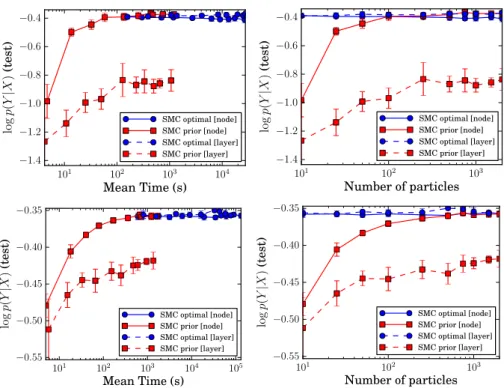
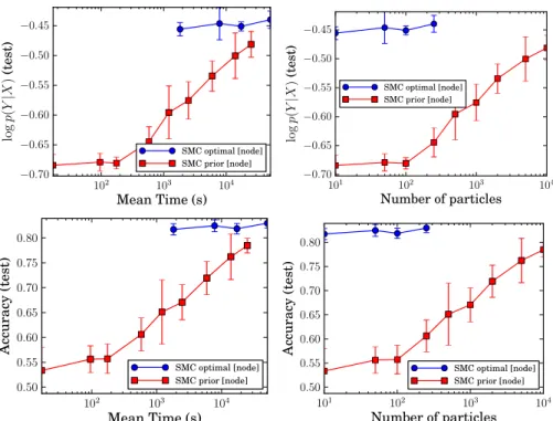
3.2 Results onpen-digits and magic-04 datasets comparing test logp(y|x) as a function of runtime and the number of particles . . . 37

3.3 Results onpen-digits andmagic-04 datasets: Test accuracy as a function of runtime and the number of particles . . . 38

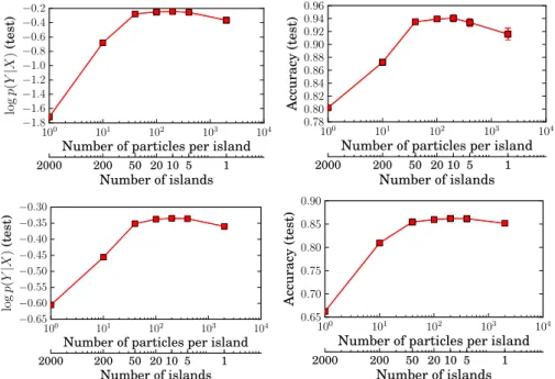
3.5 Results onpen-digits andmagic-04 dataset: Test logp(y_|x) and accuracy vs number of islands and number of particles per island . . . 38

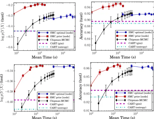
3.4 Results onmadelon dataset: Comparing logp(y|x) and accuracy on the test data against runtime and the number of particles . . . 39

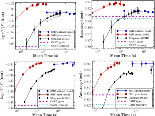
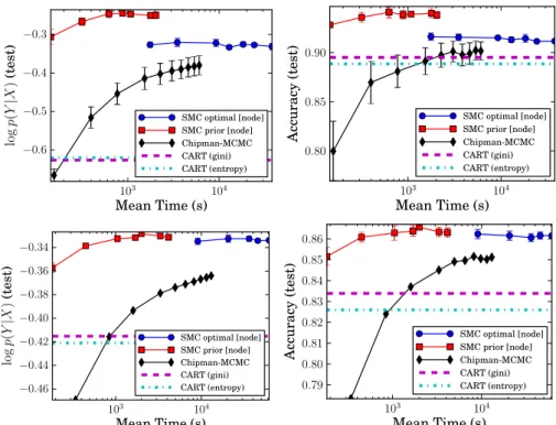
3.6 Results on pen-digits and magic-04 datasets: Test logp(y_|x) and test accuracy, vs runtime . . . 40

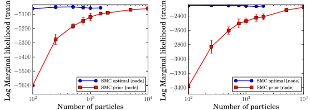
3.7 Results onpen-digits and magic-04 datasets: Mean log marginal likeli-hood vs number of particles . . . 40

3.8 Results for the following hyperparameters: α= 5.0,αs= 0.8, βs= 0.5 . 41 3.9 Results for the following hyperparameters: α= 5.0, αs = 0.95,βs= 0.2 42 3.10 Results for the following hyperparameters: α= 5.0,αs= 0.8, βs= 0.2 42 3.11 Results for the following hyperparameters: α= 1.0, αs= 0.95, βs = 0.5 43 4.1 Sample hypercube-2 dataset . . . 56

4.2 Results on Hypercube-2 dataset . . . 56

5.1 Example of a decision tree . . . 63

5.2 Online learning with Mondrian trees on a toy dataset . . . 69

5.3 Results on various datasets comparing test accuracy as a function of (i) fraction of training data and (ii) training time . . . 77

5.4 Comparison of MFs and dynamic trees . . . 78

(9)

List of tables

4.1 Comparison of ESS for CGM, GrowPrune and PG samplers on Hypercube-Ddataset. . . 58

4.2 Comparison of ESS/s (ESS per second) for CGM, GrowPrune and PG samplers on Hypercube-Ddataset . . . 58

4.3 Characteristics of datasets . . . 58

4.4 Comparison of ESS for CGM, GrowPrune and PG samplers on real world datasets . . . 59

4.5 Comparison of ESS/s for CGM, GrowPrune and PG samplers on real world datasets . . . 59

5.1 Average depth of Mondrian forests trained on different datasets . . . 77

6.1 Comparison of MFs to popular decision forests and large scale GPs on the flight delay dataset . . . 92

6.2 Comparison of calibration measures for MFs and popular decision forests on the flight delay dataset . . . 93

(10)

List of algorithms

2.1 BuildDecisionTree _D1:n,min samples split

. . . 17

2.2 ProcessBlock j,DNj,min samples split . . . 17

2.3 Predict _T,x (prediction using decision tree) . . . 18

2.4 Pseudocode for learning boosted regression trees . . . 20

3.1 SMC for Bayesian decision tree learning . . . 33

4.1 Bayesian backfitting MCMC for posterior inference in BART . . . 50

4.2 Conditional-SMC algorithm used in the PG-BART sampler . . . 54

5.1 SampleMondrianTree λ,D1:n . . . 62 5.2 SampleMondrianBlock j,_DNj, λ . . . 62 5.3 InitializePosteriorCounts(j) . . . 66 5.4 ComputePosteriorPredictiveDistribution T,G . . . 67 5.5 ExtendMondrianTree(_T, λ,_D) . . . 68 5.6 ExtendMondrianBlock(_T, λ, j,_D) . . . 68 5.7 UpdatePosteriorCounts(j, y) . . . 70 5.8 Predict _T,x (prediction using Mondrian classification tree) . . . 72

5.9 SampleMondrianBlock j,_DNj, λ version that depends on labels . . . 73

5.10 ExtendMondrianBlock(T, λ, j,D) version that depends on labels . . . 74

6.1 SampleMondrianTree _D1:n,min samples split . . . 82

6.2 SampleMondrianBlock j,_DNj,min samples split . . . 82

6.3 ExtendMondrianTree(T,D,min samples split) . . . 83

6.4 ExtendMondrianBlock(_T, j,_D,min samples split) . . . 83

6.5 Predict T,x (prediction using Mondrian regression tree) . . . 88

(11)

Chapter 1 Outline

Decision trees are a very popular tool in machine learning and statistics for prediction tasks (e.g. classification and regression). In a nutshell, learning a decision tree from training data involves two steps: (i) learning an hierarchical, tree-structured partitioning of the input space and (ii) learning to predict the label within each leaf node. During prediction stage, we simply traverse down the decision tree from the root to the leaf node and predict the label. Popular decision tree induction algorithms such as CART

(Breiman et al.,1984) and C4.5 (Quinlan,1993) have been named amongst the top 10

algorithms in data mining (Wu et al.,2008). The main advantage of decision trees is that they are computationally fast to train and test. Another advantage of decision trees is that they are well-suited for datasets with mixed attribute types (e.g. binary, categorical, real-valued attributes). Moreover, they deliver good accuracy and are interpretable (at least on simple problems), hence they are very popular in practical applications. While decision trees are powerful, they are prone to over-fitting and require heuristics to limit their complexity (e.g. limiting the maximum depth or pruning the learned decision tree on a validation data set) in order to minimize their generalization error. A useful way to think about the over fitting issue is in terms of bias variance tradeoff, using the tree depth as a complexity measure (as deeper trees can capture more complex interactions). Deep decision trees exhibit low bias as they can potentially memorize the training dataset, however they exhibit high variance, i.e. a decision tree algorithm trained on two different training datasets (from the same ‘population’ distribution) would produce very different decision trees; hence, decision trees are also referred to as

unstable learners. Another disadvantage of decision trees is that they typically do not

produce probabilistic predictions. In many applications (e.g. clinical decision making), it is useful to have a predictor that can quantify predictive uncertainty instead of just producing a point estimate. The probabilistic approach (Ghahramani,2015;Murphy,

2012) provides an elegant solution to both of these problems.

(12)

First, we introduce aprior over decision trees (e.g. a prior that prefers shallow trees) and the leaf node parameters (i.e. the parameters that predict the label within each leaf node). Next, we define alikelihood which measures how well a decision tree explains the given training data. Finally, we compute the Bayesian posterior over decision trees and the node parameters. During prediction, the predictions of trees are weighted according to their weights according to the posterior distribution. This process is known as

Bayesian model averaging (Hoeting et al., 1999) and accounts for the uncertainty in the

model (the model is the decision tree in this case) instead of picking just one decision tree. Moreover, the Bayesian approach allows us to better quantify predictive uncertainty, by translating model uncertainty into predictive uncertainty. The main disadvantage of the Bayesian approach is the computational complexity. While computing the Bayesian posterior over node parameters is fairly straightforward, computing the exact posterior distribution over trees is infeasible for non-trivial problems and in practice, we have to resort to approximations. Some early examples of Bayesian decision trees areBuntine

(1992);Chipman et al. (1998);Denison et al. (1998).

Ensemble learning (Dietterich, 2000), where we combine many predictors / learners, is another way to address over-fitting. Two popular ensemble strategies areboosting

(Schapire,1990;Freund et al.,1999) and bootstrap aggregation, more commonly referred

tobagging (Breiman,1996) . While ensemble learning can be combined with any learning

algorithm, ensembles of decision trees are very popular since decision trees are unstable learners and are computationally fast to train and test. Ensembles of decision trees often achieve state-of-the-art performance in many supervised learning problems (Caruana

and Niculescu-Mizil,2006;Fern´andez-Delgado et al.,2014). While the combination of

boosting and decision trees has been studied by many researchers (cf. (Freund et al.,

1999)), the most popular variant in practice is thegradient boosted decision trees (GBRT)

algorithm proposed byFriedman(2001). While GBRTs are popular in practice, they can over-fit and moreover, they do not produce probabilistic predictions. Chipman

et al.(2010) proposedBayesian additive regression trees (BART), a Bayesian version of

boosted decision trees. In his seminal paper,Breiman(2001) proposed random forests

(RF) which consist of multiplerandomized decision trees. Some popular strategies for randomizing the individual trees in a random forest are (i) training individual trees on bootstrapped versions of the original dataset, (ii) randomly sampling a subset of the original features before optimizing for split dimension and split location and (iii) randomly sampling candidate pairs of split dimensions and split locations and restricting the search to just these pairs. While random forests were originally proposed for supervised learning, the random forest framework is very flexible and can be extended to other problems such as density estimation, manifold learning and semi-supervised learning (Criminisi et al., 2012). Random forests are less prone to over-fitting, however they do not produce probabilistic predictions. Another disadvantage of random forests is that they are difficult to train incrementally.

(13)

and the parameters associated with the nodes of a decision tree as a probabilistic model. The probabilistic approach allows us to encode prior assumptions about tree structures and share statistical strength between node parameters. Moreover, the probabilistic approach offers a principled mechanism to obtain probabilistic predictions and quantify predictive uncertainty. The probabilistic view enables us to think about the different sources of uncertainty and understand the computational vs performance trade-offs involved in designing an ensemble of decision trees with desirable properties (high accuracy, fast predictions, probabilistic predictions, efficient online training, etc).

We make several contributions in this thesis:

• In Chapter 2, we review decision trees and set up the notation. We briefly review ensembles of decision trees, clarify what it means to be Bayesian in this context, and discuss the relative merits of Bayesian and non-Bayesian approaches.

• In Chapter 3, we first present a novel sequential interpretation of the decision tree prior and then propose a top-down particle filtering algorithm for Bayesian learning of decision trees as an alternative to Markov chain Monte Carlo (MCMC) methods. This chapter is based on (Lakshminarayanan et al., 2013), published in ICML 2013, and is joint work with Daniel M. Roy and Yee Whye Teh.

• In Chapter 4, we combine the above top-down particle filtering algorithm with the Particle MCMC framework (Andrieu et al.,2010) and propose PG-BART, a Particle Gibbs sampler for BART. This chapter is based on (Lakshminarayanan

et al.,2015), published in AISTATS 2015, and is joint work with Daniel M. Roy

and Yee Whye Teh.

• In Chapter 5, we propose a novel random forest calledMondrian forest (MF) that leverages tools from the nonparametric-Bayesian literature such as the Mondrian process (Roy and Teh, 2009) and the hierarchical Pitman-Yor process (Teh,

2006). Unlike existing random forests, Mondrian forests produce principled uncertainty estimates, and can be trained online efficiently. This chapter is based

on (Lakshminarayanan et al.,2014), published in NIPS 2014, and is joint work

with Daniel M. Roy and Yee Whye Teh.

• In Chapter 6, we extend Mondrian forests to regression and demonstrate that MFs outperform approximate Gaussian processes on large-scale regression, and produce better uncertainty estimates than popular decision forests. This chapter is based on (Lakshminarayanan et al.,2016), published in AISTATS 2016, and is joint work with Daniel M. Roy and Yee Whye Teh.

(14)

Chapter 2 Review of decision trees and

ensembles of trees

2.1 Problem setup

GivenN labeled examples (x1, y1), . . . ,(xN, yN)∈ X × Y as training data, the task in

supervised learning is to predict labelsy∈ Y for unlabeled test pointsx∈ X. Since we are interested in probabilistic predictions, our goal is to not just predict a labely_{∈ Y}, but to output the distributionp(y_|x), i.e. the conditional distribution of the label y given the featuresx. For simplicity, we assume that X :=RD, where Ddenotes the

dimensionality (i.e. the number of features), and restrict our attention to two popular supervised learning scenarios:

• multi-class classification (of whichbinary classification is a special case) where

Y :=_{1, . . . , K_} (K denotes the number of classes in this case), and

• regression where_Y :=R.

Let X1:n := (x1, . . . ,xn), Y1:n := (y1, . . . , yn), and D1:n := (X1:n, Y1:n). For every

subsetA⊆ {1, . . . , N}, letYA:={yn : n∈A} and similarly for XA and DA.

2.2 Decision trees

For our purposes, a decision tree on _X will be a hierarchical, axis-aligned, binary partitioning ofX and a rule for predicting the label of test points given training data. The structure of the decision tree is a finite, rooted, strictly binary tree T, i.e., a finite set of nodes such that 1) every node j has exactly one parent node, except for a distinguishedroot node which has no parent, and 2) every node j is the parent of exactly zero or two children nodes, called the left child left(j) and the right child right(j). Denote the leaves ofT(those nodes without children) byleaves(T). Each node

(15)

:x1>0.5 0 1 :x2>0.3 10 11 0 1 0 1 F F x2 x1 0 1 1

B

0

B

1

B

0

B

10

B

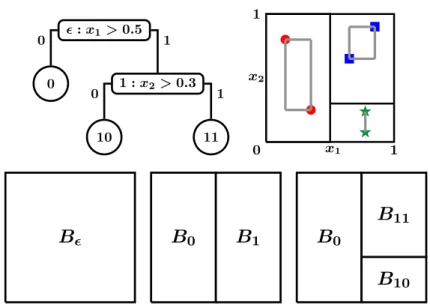
11

Figure 2.1: A decision tree_T = (T,δ,ξ) represents a hierarchical partitioning of a space. Here, the space is the unit square and the treeTcontains the nodes_{,0,1,10,11_}. The root node

represents the whole spaceB=RD, while its two children 0 and 1, represent the two halves of the cut (δ, ξ) = (1,0.5), whereδ = 1 represents the dimension of the cut, and ξ = 0.5 represents the location of the cut along that dimension. (The origin is at the bottom left of each figure, and thex-axis is dimension 1. The red circles, green stars and blue squares represent observed data points.) The second cut, (δ1, ξ1) = (2,0.35), splits the blockB1 into the two

halvesB11and B10.

When defining the prior over decision trees given byChipman et al.(1998), it will be necessary to refer to the “extent” of the data in a block. Here,Bx

j =e x

j1×exj2 denotes the bounding box

of data (shown in gray) in blockBj, whereexj1 andexj2 are theextent of the data in dimensions

1 and 2, respectively. For each nodej, the setVj contains those dimensions with non-trivial extent. Here,V0={1,2}, butV10={2}, because there is no variation in dimension 1.

of the tree j _∈ T is associated with a block Bj ⊂ RD of the input space as follows:

At the root, we have B =RD, while each internalnode j ∈T\leaves(T) with two

children represents asplitof its parent’s block into two halves, with δj ∈ {1, . . . , D}

denoting the dimension of the (axis-aligned) split, andξj denoting the location of the

split. In particular,

B_left₍_j₎:=_{x_∈Bj :xδj ≤ξj} and Bright(j) :={x∈Bj :xδj > ξj}.

We call the tuple_T = (T,δ,ξ) adecision tree. (See Figure2.1for more intuition on the representation and notation of decision trees.) Note that the blocks associated with the leaves of the tree form a partition ofRD. We may writeBj = `j1, uj1×. . .× `jD, ujD

, where`jd andujd denote the `ower and upper bounds, respectively, of the rectangular

blockBj along dimensiond. Let`j ={`j1, `j2, . . . , `jD} and uj ={uj1, uj2, . . . , ujD}.

It will be useful to introduce some additional notation. Let parent(j) denote the parent of node j. Let Nj denote the indices of training data points at node j, i.e.,

Nj ={n∈ {1, . . . , N}:xn∈Bj}. Note that bothBj andNj depend onT, although we

(16)

the`ower andupper bounds of training data points (hence the superscriptx) respectively in nodej along dimension d. Additionally, let ex

jd = (`xjd, uxjd] denote theextent of the

training data in nodej along dimensiond. LetBx

j = `xj1, uxj1 ×. . .× `x jD, uxjD ⊆Bj

denote the smallest rectangle that encloses the training data points in node j. Let leaf(x) denote the unique leaf node j _∈leaves(T) such thatx_∈Bj. (Recall that the

leaves define a partition of the input space.) For brevity, we will also use the following shortcut notation to label the nodes of the decision tree: label the root node as the empty string and label left(j) = j0 and right(j) = j1. If each parent-child path is labeled 0 or 1 depending on the outcome of the binary decision, this labeling scheme ensures that the label of each node is the concatenation of the labels along the path from the root till that node. We refer to Figure2.1for more intuition on the representation and notation of decision trees.

Once we have a decision tree structure, we also need a rule for predicting the label of a test points given training data. To this end, we will associate each leaf nodej with a parameterθj that parametrizes the conditional distributionp(y|x∈Bj). For instance,

θj would parametrize the K-dimensional discrete distribution for classification problems

and the mean of a Gaussian distribution for regression problems.

2.2.1 Learning decision trees

Learning a decision tree from training data involves two steps namely, learning the tree structureT and estimating the leaf node parametersθ. Popular decision tree induction algorithms include CART (Breiman et al., 1984) and C4.5 (Quinlan, 1993). While it is possible to learn a deep decision tree until there is an unique data point at each leaf node, it is common to limit the complexity of the decision tree by specifying a hyper-parameter that decides when to stop splitting a node. The most popular strategy is to require a minimum number of samples (min samples split) at a node before it can be split. (A variant of this strategy is to require that a split leads to a minimum number of samples min samples leaf at each leaf node.) Alternative strategies include not splitting a node if all the class labels are identical (for classification problems) or limiting the maximum depth of the tree; however specifying maximum depth is relatively harder to specify in a dataset-agnostic fashion (since deeper and/or unbalanced trees might be preferable for some datasets). Due to its simplicity and robustness, we prefermin samples split. We describe a typical decision tree induction algorithm in Algorithms 2.1 and 2.2. The procedure starts with the root node and recurses down the tree. At node j, CandidateSplits_j denotes the set of candidate pair ofvalid split dimensions and locations, where a valid split is one where both children are non-empty. In practice, the set of valid split candidates is obtained by sorting the training data independently along each dimension; since the training data takes on only along a finite number of unique values, it is sufficient to consider a single split location (usually the midpoint) for each

(17)

of these intervals (as any split location along this midpoint has the same accuracy on the training data). We greedily choose the best split dimension and split location from CandidateSplits_j by optimizing an appropriate criterion, e.g. information gain or Gini index for classification and reduction in MSE for regression.

Algorithm 2.1 BuildDecisionTree _D1:n,min samples split

1: Initialize empty tree: T=_∅,leaves(T) =_∅,δ=_∅,ξ=_∅

2: Set N={1,2, . . . , n} . entire dataset is used at root node

3: ProcessBlock ,DN,min samples split

. Algorithm 2.2

Algorithm 2.2 ProcessBlock j,_DNj,min samples split

1: Add j toT

2: if |Nj| ≥min samples split then . j is an internal node.

3: SetCandidateSplits_j to the set of all valid pairs of split dimensions and locations

4: Choose best split dimension δj and split location ξj amongst CandidateSplitsj

by optimizing appropriate criterion . greedy optimization

5: SetN_left₍_j₎={n∈N_j :X_n,δ_j ≤ξ_j}and N_right₍_j₎={n∈N_j :X_n,δ_j > ξ_j} 6: ProcessBlock left(j),DNleft(j),min samples split

7: ProcessBlock right(j),D_N_right₍_j₎,min samples split

8: else . j is a leaf node

9: Add j toleaves(T) 10: Estimateθ_j usingY_N_j

For leaf nodes, we estimate the parametersθj using DNj. In the simplest case,θj is estimated just usingYNj, independent ofXNj; there exist variants whereθjalso depends onXNj, however we restrict our attention to the former since it is computationally fast. For classification problems, letcjk denote the number of data points in node j with

labelk, i.e. cjk =P_n_∈_N_j1[yn=k]; in this case,θj is estimated as

θjk =

cjk+α

|Nj|+Kα

,

where we add a small constantα to smooth the empirical histogram of labels in node j and _|Nj|(the size of the set Nj) denotes the number of data points in node j. For

regression problems,θj is set to the empirical mean of the labels in nodej, i.e.

θj = 1 |Nj| X n∈Nj yn.

2.2.2 Prediction with a decision tree

Recall that leaf(x) denotes the unique leaf node j ∈ leaves(T) such that x ∈ Bj.

Prediction from a tree involves two steps: (i) traversing the decision tree starting from the root node to identifyleaf(x) and (ii) returning (a function of) the leaf node parameter

(18)

one can return either the probabilistic predictionθ_leaf₍_x₎ or the most likely class label argmax_kθleaf(x),k. The procedure is summarized in Algorithm 2.3.

Algorithm 2.3 Predict _T,x

(prediction using decision tree)

1: . Description of prediction using a decision tree given _T andθ

2: Initialize j= 3: while True do

4: if j∈leaves(T) then .Reached leaf(x)

5: return prediction θj

6: else

7: if x_δ_j ≤ξ_j thenj←left(j)elsej ←right(j) .recurse to child wherex lies

2.3 Bayesian decision trees

In the previous section, we described a simple tree induction procedure to learn a decision tree and the leaf node parameters. However, a potential drawback is that the greedy induction procedure can over-fit the training data, thereby leading to overconfident predictions on unseen data. Assume that the labels were generated according to a decision tree_T∗ (the ‘ground truth’). Given finite training data, the greedy learning algorithm returns an estimate Tb (a single tree) which does not equal T∗ in general.

Specifically, there are two issues: first, there could be multiple decision tree structures that are equally good at explaining the training data; however the induction algorithm returns just a single decision tree. Next, the leaf node parameters are estimated using just the data points at that leaf node; this may lead to poor generalization. Clearly, it would be desirable to represent the uncertainty over decision tree structures and the leaf node parameters.

The Bayesian approach (Bayes and Price,1763) provides a principled solution to this issue. The Bayesian approach is conceptually very simple. First, we introduce aprior

over decision trees (e.g. a prior that prefers shallow trees) and the leaf node parameters (e.g. a prior that prefers smaller values for regression or a prior that encourages sparse label distributions for classification). Next, we define alikelihood which measures how well a decision tree explains the given training data. Finally, we compute the posterior

distribution over decision trees and the node parameters using Bayes theorem:

p(T,θ|Y,X) | {z } posterior = 1 Z(Y,X) p(Y| |T{z,θ,X}) likelihood p(θ|T)p(T |X) | {z } prior , Z(Y,X) =X T Z θ p(Y|T,θ,X)p(θ|T) p(T |X)dθ,

(19)

the predictions of trees are weighted according to the posterior distribution, i.e., p(y_|x) =X T Z θ p(y_|x,_T,θ)p(_T,θ_|Y,X)dθ.

This process is known asBayesian model averaging (Hoeting et al.,1999) and accounts for the uncertainty in the model (in this case, the model is the decision tree along with the leaf node parameters), unlike the previous approach which predicts just using a single decision tree and set of leaf node parameters. The Bayesian approach allows us to quantify predictive uncertainty (by translating the model uncertainty into predictive uncertainty) which is useful in a variety of applications such as cost-sensitive decision making, reinforcement learning, etc.

The main challenge in the Bayesian approach is the computational complexity. While computing the Bayesian posterior over node parameters is typically straight forward, computing the exact posterior distribution over trees is infeasible for non-trivial problems and in practice, we have to resort to approximations. Specifically, the integral overθ

is typically easy to compute as the likelihood is assumed to belong to the exponential family distribution and the prior overθ is the corresponding conjugate prior. However, the summation over_T is computationally intractable as there are exponentially many trees. In practice, the posterior is approximated with a finite set of trees as follows:

p(y|x)≈ S X s=1 ws p(y|x,Ts), (2.1) = S X s=1 ws Z θ p(y_|x,_Ts,θ)p(θ|Y,X,Ts)dθ, where P

sws= 1. It is possible to approximate the posterior using standard tools such

as Markov chain Monte Carlo (MCMC). Some early examples of Bayesian decision trees

are Buntine (1992); Chipman et al. (1998); Denison et al. (1998). Intuitively, these

posterior approximations replace the intractable sum over trees with a finite summation by focusing only on the promising trees and ignoring trees whose posterior weights are close to zero. We discuss Bayesian decision tree algorithms in more detail in Chapter3.

2.4 Ensembles of decision trees

In ensemble learning, many ‘weak’ predictors are combined to obtain a ‘powerful’

predictor (Dietterich, 2000) that is more accurate than the individual predictors. In the simplest case, the predictions from the ensemble are just a weighted additive combination of the predictions from the individual predictors. While ensemble learning can be combined with any learning algorithm, ensembles of decision trees are very popular since decision trees are computationally fast to train and test. Ensembles of

(20)

decision trees often achieve state-of-the-art performance in many supervised learning problems (Caruana and Niculescu-Mizil,2006). Let _{Tm,θm}Mm=1 denote an ensemble of trees, whereM denotes the number of trees in the ensemble. Letg(x;Tm,θm) denote

the prediction from themth _{decision tree for a test data point}_x_{. (We slightly abuse}

the notation to allow the prediction to either be a point estimate or a probability distribution or density.) The prediction from an ensemble can be written as

g(x;{Tm,θm}Mm=1) =

M

X

m=1

wm g(x;Tm,θm). (2.2)

Ensembles of decision trees can be broadly classified into two families: additive/boosted

decision trees, wherein each tree fits the residual not explained by the remainder of the

trees, andrandom forests, wherein randomized independent decision trees are grown independently and predictions are averaged to reduce variance. We briefly review these variants below.

2.4.1 Additive decision trees

Boosting is an ensemble learning framework where each predictor is trained to focus on

the mistakes of the other predictors. Early boosting algorithms include the AdaBoost algorithm for binary classification proposed by Freund and Schapire (1997) and the

gradient boosted regression trees (GBRT) algorithm proposed byFriedman(2001) for

regression problems. An high-level pseudocode for fitting an ensemble of boosted regression trees is described in Algorithm 2.4. (Note that this is just a high-level pseudocode; it is important to prevent individual trees from overfitting cf. (Friedman,

2002).)

Algorithm 2.4 Pseudocode for learning boosted regression trees

1: Inputs: Training data (X, Y) 2: for m= 1 :M do

3: Compute residual Rm = Y −P_mm0−₌₁1 g(X;T_m0,θ_m0).

4: Learn mth decision tree T_m,θ_m usingR_m as the targets forX . Algorithm2.1

Note that the decision trees are fit in a serial fashion in Algorithm2.4. Specifically, we compute the residual, which equals the difference between the targets and the sum of predictions of all previous trees, and use this residual as the target for the mth _tree.

This depth-first expansion can lead to over-fitting. An alternative is to fit the trees in an iterative breadthwise-expansion scheme, where we fit the root of theM trees first, and subsequently fit the individual trees by expanding them, one node at a time. Examples of iteratively fitted additive regression trees include additive groves (Sorokina et al.,

2007),Bayesian additive regression trees (BART) (Chipman et al.,2010) and greedy

(21)

usually refers to serial-fitting, the termadditive decision trees includes both serial-fitting and iterative-fitting.

Chipman et al.(2010) introduced Bayesian additive regression trees (BART), which

reduce over-fitting in gradient boosted regression trees using a Bayesian approach. Similar to Bayesian decision trees discussed in Section2.3, BART introduces priors on the decision trees and leaf node parameters and approximates the posterior over the ensemble{Tm,θm}Mm=1 using an MCMC sampler. We discuss BART in more detail in Chapter4.

Caruana and Niculescu-Mizil(2006) found that boosted decision trees were slightly more

accurate than random forests. However, boosted decision trees are more sensitive to label noise. Unlike random forests, the computation across trees cannot be parallelized. Another disadvantage is that additive regression trees do not readily extend to multi-class classification problems.

2.4.2 Random forests

Classic decision tree induction procedures choose the best split dimension and location from all candidate splits at each node by optimizing some suitable quality criterion (e.g. information gain) in a greedy manner. In a random forest, the individual trees are randomized to de-correlate their predictions. The most common strategies for injecting randomness are:

• bootstrap aggregation, more commonly referred to as bagging (Breiman,1996) where each decision tree is trained on a slightly different training dataset, and

• randomly subsampling the set of candidate splits within each node.

The prediction from a random forest is usually an (unweighted) average of the predictions of individual trees: g(x;{Tm,θm}Mm=1) = M X m=1 1 M g(x;Tm,θm).

For classification, it is also possible to use majority voting if the individual trees output discrete class labels instead of probability distributions. While it is common to use uniform weights wm = M−1, the weights can also be optimized, e.g. using stacking

(Wolpert,1992).

Geurts et al.(2006) discuss the advantage of random forests over decision trees using the

bias-variance tradeoff. Individual decision trees have low bias, but exhibit high variance (as tree induction algorithms produce different trees on slightly different versions of the dataset.) In a random forest, the individual trees are randomized in order to decorrelate their predictions. The randomization scheme may slightly increase the bias

(22)

of individual trees in the forest. (For instance, if each tree of the forest is trained on a random subset of the training dataset, the individual trees may have lower accuracy than the best possible decision tree.) However, the variance of the forest is much lower than the variance of the individual trees,1 _{which more than compensates for the slight} increase in bias, thereby leading to a better predictor. Dietterich (2000) discusses three fundamental reasons why an ensemble might outperform a single classifier. The first reason is statistical: given finite training data, many hypotheses may be equally good on the training data. By combining predictions from multiple good predictors, an ensemble reduces the risk of choosing the wrong hypothesis. The second reason is computational: in cases where the training algorithm is prone to local optima, the ensemble combines the results from multiple random searches and may provide a better approximation to the true unknown function. The third reason is representational: while decision trees can represent any function in principle, the effective hypothesis space is limited by the greedy training algorithm. An ensemble is capable of representing weighted combinations of trees, which increases its effective representational power while training on finite data using a greedy local search.

Two popular random forest variants are Breiman-RF (Breiman,2001) and Extremely

randomized trees (ERT)(Geurts et al.,2006). Breiman-RF uses bagging and furthermore,

at each node, a random k-dimensional subset of the original D features is sampled. ERT chooses ak dimensional subset of the features and then chooses one split location each for thek features randomly (unlike Breiman-RF which considers all possible split locations along a dimension). Unlike Breiman-RF, ERT does not use bagging.

As we will see later, random forests are better-suited than boosted decision trees for different settings such as binary classification, multi-class classification, regression, etc. Random forests are very easy to implement as they only involve a minor change of the decision tree pseudocode. For instance, bagging just requires settingN in Algorithm2.1

to a bootstrap sample instead of the full dataset. Similarly, random split sampling just requires settingCandidateSplits_j to a subset of the valid splits in Algorithm2.2. Another advantage is that the individual trees can be trained in parallel since they do not interact with each other. Fern´andez-Delgado et al.(2014) compared a suite of machine learning algorithms on a variety of datasets and found that random forests consistently rank among the top-performing algorithms. Due to these advantages, random forests remain one of the most popular black-box prediction algorithms. We refer the reader to

(Criminisi et al., 2012) for an excellent review of random forests and other extensions

such as density estimation, manifold learning and semi-supervised learning.

While the random forest framework is very powerful, it has a couple of disadvantages. First, random forests do not quantify predictive uncertainty in a principled way. Specifi-cally, methods such as Gaussian processes have the appealing property that uncertainty

1

Specifically, the variance of a forest withM trees isM times lower than the variance of individual trees.

(23)

increases as we move farther away from the training data. However, predictions from a random forest can be over-confident even in regions where training data has not been observed. The main reason for this difference is that Gaussian processes are probabilistic whereas random forests are not. In a probabilistic framework, we first posit a prior that represents our uncertainty about the parameters of the underlying function, and next posit a likelihood function that measures how well the parameters explain the observed training data. Finally, we compute the predictive posterior using Bayes theorem. The observed data constrains the function by down-weighting unlikely parameters; hence the predictive posterior is less uncertain in regions close to the observed training data. However, the observed training data does not constrain the function in regions far away from the training data, hence the predictive posterior reduces to the prior distribution and exhibits higher uncertainty (as expected) in regions far from the observed training data.

Another disadvantage of random forests is that they are not well suited for incremental

or online learning setting where we observe new data points on-the-fly (unlike the

batch learning setting where the training dataset does not grow with time.) Large-scale

machine learning systems for streaming data are often trained using stochastic gradient algorithms. However, random forests with hard splits are not amenable to gradient based updates. Since it is difficult to undo splits in decision trees, current online random forests wait until they have seen sufficient amount of data to confidently decide the split. Hence, they are very data inefficient compared to the corresponding batch random forest. We propose a novel variant of random forests that addresses both of these issues in Chapters5and 6.

2.5 Bayesian model averaging vs model combination

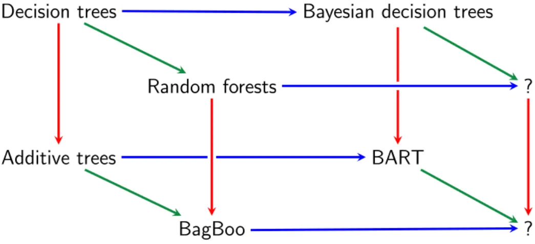
We have discussed several algorithms so far. In this section, we discuss the connections between the different algorithms and clarify the differences between seemingly similar approaches. The connections between the algorithms are summarized in Figure2.2. We start with decision trees on the top left corner of Figure2.2. Red lines indicate additive combination (or boosting), where the components are fit jointly in a serial fashion; for instance additive trees combine decision trees. Green lines indicate ran-domized averaging where multiple ranran-domized versions of the underlying predictor are trained in parallel and their predictions are averaged; for instance random forests average predictions from multiple randomized decision trees. It is possible to apply combine bagging and boosting;Pavlov et al. (2010) proposed BagBoo, where multiple randomized versions of boosted decision trees are fit in parallel and averaged. Blue lines indicate Bayesian treatment of the decision tree structures and the leaf node parameters. As the name suggests, Bayesian decision trees perform BMA over decision trees, whereas BART performs Bayesian inference over additive combination of decision trees.

(24)

Decision trees

Bayesian decision trees

Random forests

?

Additive trees

BART

BagBoo

?

Figure 2.2: Comparison of different approaches: blue horizontal lines denote Bayesian version, red vertical lines denote additive combination, and green lines denote an ensemble combination of randomized predictors. The top-down particle filtering algorithm described in Chapter3is a novel Bayesian decision tree variant (top right node). The PG-BART algorithm described in Chapter4is a novel variant of BART (and Bayesian decision trees). Mondrian forests, described in Chapters5 and6, are a novel hybrid variant of random forests, where we perform Bayesian inference over node parameters in each tree but combine the trees in a non-Bayesian fashion. Furthermore, in Mondrian forests, we restrict splits to the range of observed training data, which allows us to represent uncertainty about the partition structure beyond the range of training data.

Equation (2.1) describing BMA in Bayesian decision trees and equation (2.2) describing the prediction of an ensemble appear to be strikingly similar. It seems tempting to interpret BMA as an ensemble algorithm, however the goals of BMA are quite different.

Domingos(2000) interpreted BMA as an ensemble method and claimed that BMA is

prone to over-fitting, howeverMinka(2000) showed that the ensemble interpretation of BMA is incorrect. Ensembles performmodel combination and hence their hypothesis class is bigger. On the other hand, BMA in Bayesian decision trees assumes that the data was generated by a decision tree and accounts for the uncertainty over trees due to the fact that we observe only finite training data. On finite data, BMA performs

soft model selection instead of model combination. In fact, in the limit of infinite

data, the Bayesian posterior over decision trees would converge to a single tree and only one of the weights in (2.1) would be non-zero. If the data was generated by an ensemble of trees instead of a single decision trees, Bayesian decision trees would not be appropriate as the assumptions of BMA are violated. (We refer to (Minka,2000) for a simple illustration of the difference between model combination and BMA.Clarke

(2003) provides a comparison between BMA and ensemble weighting when the model approximation error cannot be ignored.) The correct solution is to assume that the data was generated by an additive combination of trees and perform BMA over additive combinations of trees instead of BMA over decision trees. In fact, this is the approach taken in BART (Chipman et al., 2010), as we will see in Chapter 4. It is possible to interpolate between BMA over decision trees (where each tree is weighted by its posterior probability) and random forests (where the trees are weighted uniformly).

(25)

Quadrianto and Ghahramani (2015) propose to use power likelihood which enables interpolation between Bayesian model averaging and model combination.

It is important to note that the term ‘Bayesian’ in Bayesian decision trees refers to Bayesian inference over both the decision tree structuresand the leaf node parameters. In Chapters5 and6, we discussMondrian forests, where we perform Bayesian inference over leaf node parameters but combine the decision trees in a non-Bayesian fashion using model combination instead of BMA. Furthermore, in Mondrian forests, we restrict splits to the range of observed training data, which allows us to represent uncertainty about the partition structure beyond the range of training data. Mondrian forests use a hierarchy over the node parameters, conditional on the tree structure, and use Bayesian inference within each tree independently to obtain probabilistic predictions. Since splits are confined to bounding boxes, we can represent uncertainty in the tree structure in regions far away from training data; hierarchical Bayesian inference over node parameters ensures that we efficiently make use of observed training data. Hence, Mondrian forests can produce principled uncertainty estimates. Taddy et al. (2015) proposeBayesian and empirical Bayesian forests, where the bootstrap in random forest is replaced by the Bayesian bootstrap (Rubin et al.,1981); however, they do not perform Bayesian inference over the decision trees and leaf node parameters. The real challenge of Bayesian inference in trees and ensembles is Bayesian inference over (exponentially many) decision trees, hence we do not refer to a decision tree (or forest) algorithm as ‘Bayesian’ unless it learns the posterior over decision trees. Bayesian inference over tree structures is computationally challenging the in incremental/online learning setting; Mondrian forests do not perform Bayesian inference over tree structures, which is part of the reason why they are computationally attractive in this setting.

Decision trees are also reminiscent of so-called mixture of experts (Jacobs et al.,1991), which learn multiple predictors (experts) and additionally learn to use a different predictor for different subsets of data. Decision trees with hard splits learn both the partitioning tree structure as well as the predictors at the leaf nodes, which are the experts in this case. It is also possible to replace the hard splits in a decision tree with soft routing functions that route each data point to the left or right stochastically. Hierarchical mixture of experts (HMEs) (Jordan and Jacobs, 1994) parametrize the routing function using sigmoid functions, and learn the parameters using expectation-maximization algorithm. One issue with the soft routing operation is that a data point needs to be propagated to every leaf, which destroys the computational advantage for deep trees. However, the sigmoid is differentiable which makes it amenable to gradient based end-to-end training. It would be interesting to develop efficient Bayesian versions of HMEs; however, we restrict our attention to decision trees with hard axis-aligned splits in the rest of the thesis.

(26)

Chapter 3 SMC for Bayesian decision trees

3.1 Introduction

Decision tree learning algorithms are widely used across statistics and machine learning, and often deliver near state-of-the-art performance despite their simplicity. Decision trees represent predictive models from an input space, typicallyRD, to an output space

of labels, and work by specifying a hierarchical partition of the input space into blocks. Within each block of the input space, a simple model predicts labels.

In classical decision tree learning, a decision tree (or collection thereof) is learned in a greedy, top-down manner from the examples. Examples of classical approaches that learn single trees include ID3 (Quinlan,1986), C4.5 (Quinlan,1993) and CART

(Breiman et al.,1984), while methods that learn combinations of decisions trees include

boosted decision trees (Friedman,2001), random forests (Breiman,2001), and many others.

Bayesian decision tree methods, like those first proposed byBuntine(1992), Chipman

et al.(1998), Denison et al. (1998), and Chipman and McCulloch (2000), and more

recently revisited byWu et al.(2007), Taddy et al.(2011) andAnagnostopoulos and

Gramacy(2012), cast the problem of decision tree learning into the framework of Bayesian

inference. In particular, Bayesian approaches start by placing a prior distribution on the decision tree itself. To complete the specification of the model, it is common to associate each leaf node with a parameter indexing a family of likelihoods, e.g., the means of Gaussians or Bernoullis. The labels are then assumed to be conditionally independent draws from their respective likelihoods. The Bayesian approach has a number of useful properties: e.g., the posterior distribution on the decision tree can be interpreted as reflecting residual uncertainty and can be used to produce point and interval estimates. On the other hand, exact posterior computation is typically infeasible and so existing approaches use approximate methods such as Markov chain Monte Carlo (MCMC) in the batch setting. Roughly speaking, these algorithms iteratively improve a complete

(27)

decision tree by making a long sequence of random, local modifications, each biased towards tree structures with higher posterior probability. These algorithms stand in marked contrast with classical decision tree learning algorithms like ID3 and C4.5, which rapidly build a decision tree for a data set in a top-down greedy fashion guided by heuristics. Given the success of these methods, one might ask whether they could be adapted to work in the Bayesian framework.

We present such an adaptation, proposing a sequential Monte Carlo (SMC) method for approximate inference in Bayesian decision trees that works by sampling a collection of trees in a top-down manner like ID3 and C4.5. Unlike classical methods, there is no pruning stage after the top-down learning stage to prevent over-fitting, as the prior combines with the likelihood to automatically cut short the growth of the trees, and resampling focuses attention on those trees that better fit the data. In the end, the algorithm produces a collection of sampled trees that approximate the posterior distribution. While both existing MCMC algorithms and our novel SMC algorithm produce approximations to the posterior that are exact in the limit, we show empirically that our algorithms run more than an order of magnitude faster than existing methods while delivering the same predictive performance.

The chapter is organized as follows: we begin by describing the Bayesian decision tree model precisely in Section3.2, and then describe the SMC algorithm in detail in Section3.3. Through a series of empirical tests, we demonstrate in Section 3.4 that this approach is fast and produces good approximations. We conclude in Section3.5 with a discussion comparing this approach with existing ones in the Bayesian setting, and point towards future avenues.

3.2 Model

3.2.1 Problem setup

We assume that the training data consist of N i.i.d. samples X = {xn}Nn=1, where

xn ∈RD, along with corresponding labels Y ={yn}Nn=1, where yn ∈ {1, . . . , K}. We

focus only on the multi-class classification task here, although the extension to regression is fairly straightforward. We refer to Section2.2and Figure2.1for a review of decision trees and our notation.

(28)

3.2.2 Likelihood model

Conditioned on the examplesX, we assume that the joint densityp(Y,T |X) of the labelsY and the latent decision tree T factorizes as follows:

p(Y,_{T |}X) =p(_{T |}X)p(Y _{| T},X) =p(_{T |}X)Q

j∈leaves(T)`(YNj|XNj) (3.1) where` denotes a likelihood, defined below.

In this chapter, we focus on the case of categorical labels taking values in the set

{1, . . . , K_}. It is natural to take ` to be the Dirichlet-Multinomial likelihood, corre-sponding to the data being conditionally i.i.d. draws from a multinomial distribution on

{1, . . . , K} with a Dirichlet prior. In particular,

`(YNj|XNj) = Γ(α) Γ(α K)K QK k=1Γ(cjk+_Kα) Γ(PK k=1cjk+α) , (3.2)

where cjk denotes the number of labels yn = k among those n ∈ Nj and α is the

concentration parameter of the symmetric Dirichlet prior. Generalizations to other likelihood functions based on conjugate pairs of exponential families are straightforward.

3.2.3 Sequential generative process for trees

The final piece of the model is the prior density p(T |X) over decision trees. In order to make straightforward comparisons with existing algorithms, we adopt the model proposed by Chipman et al.(1998). In this model, the prior distribution of the latent tree is definedconditionally on the given input vectorsX (see Section3.5for a discussion of this dependence onX and its effect on the exchangeability of the labels). Informally, the tree is grown starting at the root, and each new node either splits and grows two children (turning the node into an internal node) or stops (leaving it a leaf) stochastically and independently.

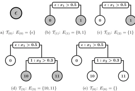
We now describe the generative process more precisely in terms of a Markov chain capturing the construction of a decision tree in stages, beginning with the trivial tree T₍₀₎ ={}containing only the root node, and sampling a sequence of partial trees. Let E₍_t₎ denotes the ordered set containing the list of nodeseligible for expansion at staget (These are the leaf nodes fromT(t−1) that have not been expanded yet.) At each stage t,T₍_t₎ is produced from T₍_t₋₁₎ by choosing one eligible node in E(t) and either growing two children nodes or stopping the leaf. Once stopped, a leaf is ineligible for future growth. The identity of the chosen leaf isdeterministic, while the choice to grow or stop isstochastic. The process proceeds until all leaves are stopped, and so each node is considered for expansion exactly once throughout the process. This will be seen to give rise to a finite sequence of decision treesT(t)= (T(t),δ(t),ξ(t)) once we define the

(29)

associated cut functionsδ₍_t₎ andξ₍_t₎. We will use this Markov chain in Section 3.3as scaffolding for a sequential Monte Carlo algorithm. A similar approach was employed by

Taddy et al.(2011) in the setting of online Bayesian decision trees. There are similarities

also with thebottom-up SMC algorithms by Teh et al.(2008) andBouchard-Cˆot´e et al.

(2012).

We next describe the rule for stopping or growing nodes, and the distribution of cuts. Letj be the node chosen at some stage of the generative process. If the input vectors

XNj are all identical, then the node stops and becomes a leaf. (Chipman et al.(1998) chose this rule because no choice of cut to the block Bj would result in both children

containing at least one input vector.) Otherwise, letVj be the set of dimensions along

which XNj varies, and let e

x

j,d = [`xj,d, uxj,d] be the extent of the input vectors along

dimensiond∈ Vj. (See last subfigure of Figure 2.1.) Under the Chipman et al. model,

the probability that nodej is split is αs

(1 +depth(j))βs , αs∈(0,1), βs∈[0,∞), (3.3) wheredepth(j) is the depth of the node, andαs andβs are parameters governing the

shape of the resulting tree. For largerαsand smallerβsthe typical trees are larger, while

the deeperj is in the tree the less likely it will be cut. If j is cut, the dimensionδj and

then location ξj of the cut are sampled uniformly fromVj andex_j,δ_j, respectively. Note

that the choice for the support of the distribution over cut dimensions and locations are such that both children ofj will, with probability one, contain at least one input vector. Finally, the choices of whether to grow or stop, as well the cut dimensions and locations, are conditionally independent across different subtrees. Figure3.1presents a cartoon of the sequential generative process.

To complete the generative model, we defineT=Tη, δ=δη andξ=ξη, where η is the

first stage such that all nodes are stopped. We note that η <2N with probability one because each cut of a nodej produces a non-trivial partition of the data in the block, and a node with one data point will be stopped instead of cut. The conditional density of the decision treeT = (T,δ,ξ) can now be expressed as

p(T,δ,ξ_|X) = Y j∈leaves(T) 1₋ αs (1 +depth(j))βs 1(|Vj|>0) × Y j∈T\leaves(T) αs (1 +depth(j))βs 1 |Vj| 1 |ex j,δj| . (3.4)

Note that the prior distribution of _T does not depend on the deterministic rule for choosing a leaf at each stage. However this choice will have an effect on the bias and variance of the corresponding SMC algorithm.

(30)

(a)T(0): E(0)={} :x1>0.5 0 1 (b) T(1): E(1)={0,1} :x1>0.5 0 1 (c)T(2): E(2)={1} :x1>0.5 0 1 :x2>0.3 10 11 (d) T(3): E(3)={10,11} :x1>0.5 0 1 :x2>0.3 10 11 (e)T(6): E(6)={}

Figure 3.1: Sequential generative process for decision trees: Nodeseligible for expansion are denoted by the ordered setE and shaded in gray. In every iteration, the first element ofE, say

j, is popped and is stochastically assigned to be an internal node or a leaf node with probability given by (3.3) At iteration 0, we start with the empty tree andE=_{_}. At iteration 1, we pop

fromE and assign it to be an internal node with split dimensionδ= 1 and split location ξ= 0.5 and append the child nodes 0 and 1 toE. At iteration 2, we pop 0 fromE and set it to a leaf node. At iteration 3, we pop 1 fromE and set it to an internal node, split dimension

δ1 = 2 and threshold ξ1 = 0.3 and append the child nodes 10 and 11 to E. At iterations 4

and 5 (not shown), we pop nodes 10 and 11 respectively and assign them to be leaf nodes. At iteration 6,E=_{}and the process terminates. By arranging the random variables ρandδ, ξ

(31)

3.3 Sequential Monte Carlo (SMC) for Bayesian decision

trees

In this section we describe an SMC algorithm for approximating the posterior distribution over the decision tree (T,δ,ξ) given the labeled training data (X, Y). (We refer the reader to (Capp´e et al., 2007) for an excellent overview of SMC techniques.) The approach we will take is to perform particle filtering following the sequential description of the prior. In particular, at staget, the particles approximate a modified posterior distribution where the prior on (T,δ,ξ) is replaced by the distribution of (T₍_t₎,δ₍_t₎,ξ₍_t₎), i.e., the process truncated at staget.

Recall thatE(t) denotes the ordered set of unstopped leaves at stage t, all of which are eligible for expansion. We refer to these nodes as candidates as they are eligible for expansion. An important freedom we have in our SMC algorithm is the choice of which candidate leaf, or set C(t)⊆E(t) of candidate leaves, to consider expanding. In order to avoid “multipath” issues (Del Moral et al., 2006, _§3.5) which lead to high variance, we fix a deterministic rule for choosing_C₍t)⊆E(t). (Multiple candidates are expanded or stopped in turn, independently.) This rule can be a function of (X, Y) and the state of the current particle, as the correctness of resulting approximation is unaffected. We evaluate two choices in experiments: first, the rule_C₍t)=E(t) where we consider expanding all eligible nodes; and second, the rule whereC(t) contains a single node chosen in a breadth-first (i.e., oldest first) manner fromE₍_t₎. (We consider only breadth-first expansion as it closely resembles top-down tree induction algorithms and allows us to interpret (t) as a surrogate for complexity of the tree.)

We may now define the sequence (PY₍_t₎) oftarget distributions. Recall the sequential

process defined in Section 3.2. If the generative process for the decision tree has not completed by staget, the process has generated (T(t),δ(t),ξ(t)) along withE(t), capturing which leaves inT₍_t₎ have been considered for expansion in previous stages already and which have not. Let _T₍t) = (T(t),δ(t),ξ(t), E(t)) be the variables generated on stage t, and write P for the prior distribution on the sequence (T(t)). We construct the target distribution PY₍_t₎ as follows: Given T(t), we generate labels Y0 with likelihood p(Y0_|T₍t),X), i.e., as if (T(t),δ(t),ξ(t)) were the complete decision tree. We then define PY₍_t₎ to be the conditional distribution ofT(t) givenY0 =Y. That is,PY₍_t₎ is the posterior

with a truncated prior.

In order to complete the description of our SMC method, we must defineproposal kernels(Q(t)) that sample approximations for thetth stage given values for the (t−1)th stage. As with our choice of C(t), we have quite a bit of freedom. In particular, the proposals can depend on the training data (X, Y). An obvious choice is to take Q(t) to be the conditional distribution of T(t) given T(t−1) under the prior, i.e., setting Q(t)(T(t)| T(t−1)) =P(T(t)| T(t−1)).

(32)

Informally, this choice would lead us to propose extensions to trees at each stage of the algorithm by sampling from the prior, so we will refer to this as theprior proposal kernel (aka the Bayesian bootstrap filter (Gordon et al.,1993)).

We consider two additional proposal kernels: The first,

Q(t)(T(t)| T(t−1)) =PY(t)(T(t)| T(t−1)), (3.5) is called the (one-step) optimal proposal kernel because it would be the optimal kernel assuming that the tth stage were the final stage. We return to discuss this kernel in Section3.3.1. The second alternative, which we will refer to as theempirical proposal kernel, is a small modification to the prior proposal, differing only in the choice of the split pointξ. Recall that, in the prior, ξ₍_t₎_,j is chosen uniformly from the intervalex

j,δj. This ignores the empirical distribution given by the input data XNj in the partition. We can account for this by first choosing, uniformly at random, a pair of adjacent data points along feature dimension δ₍_t₎_,j, and then sampling a cutξ₍_t₎_,j uniformly from the interval between these two data points.

The pseudocode for our proposed SMC algorithm is given in Algorithm 3.1. Note that the SMC framework only requires us to compute the density of_T₍_t₎ under the target distribution up to a normalization constant. In fact, the SMC algorithm produces an estimate of the normalization constant, which, at the end of the algorithm, is equal to the marginal probability of the labels Y given X, with the latent decision tree

T marginalized out. In general, the joint density of a Markov chain can be hard to compute, but because the set of nodesC(t) considered at each stage is a deterministic function of_T₍_t₎, the path (_T0,T1, . . . ,T(t−1)) taken is a deterministic function of T(t). As a result, the joint density is simply a product of probabilities for each stage. The same property holds for the proposal kernels defined above because they use the same candidate set_C₍_t₎, and have the same support as P. These properties justify equations

(3.6) and (3.7) in Algorithm3.1.

3.3.1 The one-step optimal proposal kernel

In this section we revisit the definition of the one-stepoptimal proposal kernel. While

the prior and empirical proposal kernels are relatively straightforward, the one-step

optimal proposal kernel is defined in terms of an additional conditioning on the labels

Y, which we now study in greater detail.

Recall that the one-step optimal proposal kernel Q(t) is given by Q(t)(T(t)| T(t−1)) = PY₍_t₎(T(t)| T(t−1)). To begin, we note that, conditionally onT(t−1) andY, the subtrees rooted at each nodej ∈ C(t−1) are independent. This follows from the fact that the likelihood ofY given T(t) factorizes over the leaves. Thus, the proposal’s probability