Learning Deep Models with Linguistically-Inspired Structure

LEARNING DEEP MODELS WITH

LINGUISTICALLY-INSPIRED STRUCTURE

A Dissertation

Presented to the Faculty of the Graduate School of Cornell University

in Partial Fulfillment of the Requirements for the Degree of Doctor of Philosophy

by Vlad Niculae

LEARNING DEEP MODELS WITH LINGUISTICALLY-INSPIRED STRUCTURE

Vlad Niculae, Ph.D. Cornell University 2018

Many applied machine learning tasks involve structured representations. This is particularly the case in natural language processing (NLP), where the discrete, compositional nature of words and sentences leads to natural combinatorial rep-resentations such as trees, sequences, segments, or alignments, among others. It is no surprise that structured output models have been successful and popular in NLP applications since their inception. At the same time, deep, hierarchical neural networks with latent representations are increasingly widely and success-fully applied to language tasks. As compositions of differentiable building blocks, deep models conventionally perform smooth, soft computations, resulting in dense hidden representations. In this work, we focus on models withstructure and sparsityin both theiroutputsas well as theirlatent representations, without sacrificing differentiability for end-to-end gradient-based training. We develop methods for sparse and structured attention mechanisms, for differentiable sparse structure inference, for latent neural network structure, and for sparse structured output prediction. We find our methods to be empirically useful on a wide range of applications including sentiment analysis, natural language inference, neural machine translation, sentence compression, and argument mining.

BIOGRAPHICAL SKETCH

Vlad Niculae was born in Bucharest, Romania. He obtained a Bachelor’s degree and a Master’s degree in Computer Science from the University of Bucharest, where he developed an interest for natural language processing. He then pursued the Eras-mus Mundus International Masters in Natural Language Processing and Human Language Technologies, spending one year at the University of Wolverhampton, and one year at the University of the Franche-Comté in Besançon.

Vlad is an accomplished open-source developer, a core contributor to the scikit-learnmachine learning library, and lead developer of thepolylearnlibrary for factorization machines and polynomial networks, in addition to the open-source research code for the projects he has lead throughout his Ph.D. Vlad also enjoys movies, especially those depicting the everyday, and sometimes playsBelle & Sebastiansongs on guitar.

ACKNOWLEDGEMENTS

I am infinitely grateful to Claire, my advisor, for all of the help, support, patience, and ideas. I am equally thankful for my amazing minor advisors, Sabine, and Karthik. Part of this work was done during an internship at NTT with Mathieu, who gave me the courage to venture into new territories; many results later came from collaboration with André. I am happy without bounds to have become, from a big fan of your work, to collaborator. A proto-proof of Theorem3.4came up during a dinner conversation with Noelle. Uncountable thanks to Liviu, who introduced me to NLP research. Throughout the years, I have been blessed with fantastic friends, collaborators, and co-authors, namely:

Ithaca. Ana, Andreas, Andrew, Arzoo, Basu, Chenhao, Cristian, Danlu, Eleanor, Esin, Ethan, Felix, Isaac, Jack, Jon, Joshua, Justine, Kai, Laure, Lillian, Mark, Matt, Moontae, Natacha, Ozan, Rahmtin, Rishi, Sander, Shannon, Steffen, Sydney, Tianze, Tobias, Xanda, Xilun, Yao, Yiqing;

Nara. Antoine, David, Iwata-san, Juan, Katka, Michael, Otsuka-san, Ueda-san; Saarbrücken. Anna, Beta, Bilal, Bimal, Ernesto, Eslam, Filip, Flor, Georg, Ghaz-ale, Janno, Maëva, Marcos, Pedro, Przemek, Rafaella, Raul, Scott, Tahleen, Tine;

Elsewhere. Alex, Alexandra, Alina, Alison, Anca, Andrei, Anubhav, Bo, Bob, Calvin, Daniel, Emanuela, Fabian, Farid, Gaël, Gabriela, Iuliana, Jordan, Kelly, José, Lena, Maria, Miguel, Oana, Oda, Olivier, Răzvan, Radu, Raluca, Sashko, Sever, Silvia, Srijan, Tim, Vedrana, Weronika, Wilker, among others. I am also grateful to open-source developers and graduate student unions worldwide.

TABLE OF CONTENTS

Biographical Sketch . . . iii

Dedication . . . iv

Acknowledgements . . . v

Table of Contents . . . vi

List of Tables. . . viii

List of Figures . . . ix

Notation . . . xii

1 Introduction 1 1.1 Structure in Natural Language Processing . . . 1

1.2 Contributions . . . 4

1.3 Roadmap . . . 7

2 Background 8 2.1 Machine Learning with Hidden Representations of Language . . . . 8

2.2 Convex Analysis . . . 11

2.3 Sparsity, Structured Sparsity, and Parsimony . . . 14

3 Structured Sparsity for Attention Mechanisms 19 3.1 Motivating Structured Sparsity For Attention . . . 19

3.2 Regularized max Operators . . . 23

3.3 Recovering Known Mappings and Characterizing Sparsity . . . 26

3.4 Algorithms for General Differentiable Regularizers . . . 28

3.5 Fusedmax and Oscarmax: Clustered Attention . . . 30

3.6 Experimental Results . . . 35

3.7 Discussion and Related Work . . . 41

3.8 Chapter Summary . . . 45

4 SparseMAP: Differentiable Sparse Structured Inference 46 4.1 Structured Inference Preliminaries. . . 46

4.2 Sparse Structured Inference . . . 53

4.3 ComputingSparseMAP . . . 55

4.4 Backward Pass Computation . . . 59

4.5 Sparse Alignment for Natural Language Inference . . . 61

4.6 Discussion and Related Work . . . 66

4.7 Chapter Summary . . . 67

5 Dynamically Inferred Neural Network Structure 69 5.1 Overview and Related Work . . . 69

5.2 Models with Latent Structured Variables . . . 71

5.3 Latent Dependency TreeLSTM . . . 75

5.4 Experiments . . . 75

6 SparseMAP losses for sparse structured prediction 80

6.1 Structured Prediction Losses . . . 80

6.2 A Fenchel-Young Family of Losses . . . 83

6.3 Sparse Dependency Parsing withSparseMAPLosses . . . 87

6.4 Related Work . . . 90

6.5 Chapter Summary . . . 91

7 Mining argument structures with expressive factor graphs 93 7.1 Argumentation and Argument Mining . . . 93

7.2 Argumentation Data . . . 96

7.3 Related Work . . . 98

7.4 Factor Graphs for Argument Structure Prediction . . . 99

7.5 RNN and Linear Parametrizations. . . 105

7.6 Experiments . . . 108

7.7 Error Analysis . . . 111

7.8 Chapter Summary . . . 115

8 Conclusions 116 8.1 Summary and Discussion . . . 116

8.2 Future Directions . . . 117

A Proofs 119 A.1 Sparsity of attention mappings: Proof of Proposition 3.1 . . . 119

A.2 Jacobian for general differentiableΩ: Proof of Proposition 3.2 . . . 120

A.3 Fusedmax and Oscarmax Jacobian: Proof of Proposition 3.4 . . . 121

A.4 Computing the SparseMAP Jacobian: Proof of Proposition 4.1 . . . 124

A.5 Distribution-wise SparseMAP Jacobian: Proof of Proposition 5.1 . . 126

A.6 Properties of Fenchel-Young Losses: Proof of Proposition 6.1 . . . . 127

B Implementation details 130 B.1 Conditional Gradient Algorithms forSparseMAP . . . 130

LIST OF TABLES

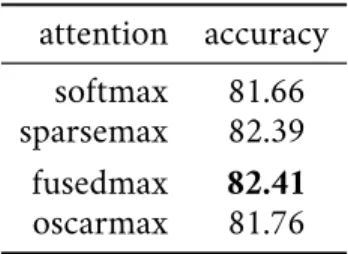
3.1 Natural language inference test accuracy on SNLI. . . 36

3.2 Sentence summarization: ROUGE-L precision, recall and F-scores. 41

3.3 Neural machine translation results: tokenized BLEU test scores. . . 42

4.1 Test accuracy scores for natural language inference with structured and unstructured variants of ESIM. In parentheses: the percentage

of pairs of words with nonzero alignment scores. . . 65

5.1 Test accuracy for classification and natural language inference. . . . 77

5.2 Results on the reverse dictionary lookup task (Hill et al., 2016). Fol-lowing the authors, for an input definition, we rank a shortlist of approximately 50k candidate words according to the cosine simi-larity to the output vector, and report median rank of the expected word, accuracy at 10, and at 100. . . 78

6.1 Unlabeled attachment accuracy scores for dependency parsing, us-ing a bi-LSTM model (Kiperwasser and Goldberg, 2016).SparseMAP

and m-SparseMAPyield the best parser on4_{/5datasets. For context,} we include the scores of the CoNLL 2017 UDPipe baseline, trained under the same conditions (Straka and Straková, 2017). . . 87

7.1 Instantiation of model design choices for each dataset. . . 103

7.2 Test set F1 scores for link and proposition classification, as well as their averages. The number of test instances is shown in paren-theses; best scores on overall tasks are in bold. Scores are micro-averaged at the document level.. . . 110

LIST OF FIGURES

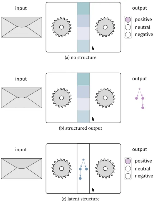
1.1 High-level view ofdeepmachine learning models for NLP, with a hidden representationhemphasized: (a) a vanilla sentiment clas-sifier, with unstructured hidden layers (typically, vector represen-tations consisting of real numbers); (b) a structured-output model

(e. g., a parser); (c) a deep model with latent structure. . . 3

2.1 ℓpnorm ballsBk·k_p in a two-dimensional space, for several values

of p. The legend matches the outside-to-inside ordering of the contours. For p < 1,ℓp are not proper norms; as p → 0the limit

vectors have exactly one nonzero coordinate. . . 15

2.2 When optimizing a linear function (left) or a quadratic function

(right) over theℓ1 ball, solutions are likely sparse. . . 16 3.1 A generic attention mechanism computes a representative vector_h¯

as a context-dependent weighted average of a sequence of vectors (hi), by inducing a probability distribution over them, i. e., h¯ = Í

i pihi. For different contexts cand c′, the distributions pand p′

may be wildly different. . . 20

3.2 Traditionally, attention mechanisms use softmax for mapping scores to probabilities, yielding dense, not very interpretable results (3.2a). Within our framework, we can derive attention mechanisms that yield sparse, clustered probabilities, aiding interpretability (3.2b).. . 22

3.3 Finding the maximum coordinate of a vector (here, θ= [.5,1,0]) is

equivalent to maximizing a linear function over the simplex. As the simplex is non-empty, a solution is always achieved at a vertex. . . . 23

3.4 The proposedmaxΩ(θ)operator up to a constant (left) and theΠΩ(θ)

mapping (right), illustrated for θ = [t,0]. In this case, maxΩ(θ)is

hinge-shaped andΠΩ(θ)is sigmoid-shaped. Our framework

recov-erssoftmaxandsparsemax. . . 26

3.5 Contour plots of attention mechanisms on the simplex. From top to bottom: softmax, sparsemax, fusedmax and oscarmax. Left column: contours of−Ω. Right column: contours off(p)₌ p⊤θ−Ω(p), and the optimalp⋆_{, for}

θ =[.8,1,0]. . . 32

3.6 3-d visualization ofΠΩ([t1,t2,0])2for several proposed and existing mappingsΠΩ. sq-pnorm-max with p = 1.5resembles sparsemax

but with smoother transitions. The proposed structured attention mechanisms, fusedmax and oscarmax, exhibit plateaus and ridges

in areas where weights become fused together. . . 33

3.7 Attention weights for the contradicted hypothesis “No one is dancing.” 37

3.8 Attention weights for French to English translation. Within a row, weights grouped by oscarmax under the same cluster are denoted by “•”. Here, oscarmax finds a slightly more natural English translation. 39

4.1 Illustration of useful structures, along with their matrix representa-tion.. . . 49

4.2 Geometrical interpretation of various inference strategies. Left: in the unstructured case,softmaxandsparsemaxcan be interpreted as regularized, differentiablearg maxapproximations;softmaxreturns dense solutions whilesparsemaxfavors sparse ones. Right: in this work, we extend this view tostructuredinference, which consists of optimizing over a polytopeM, the convex hull of all possible

structures (depicted: the arborescence polytope, whose vertices are trees). We introduce SparseMAPas a structured extension of

sparsemax: it is situated in between MAP inference, which yields a single structure, and marginal inference, which returns a dense combination of structures. . . 54

4.3 Comparison of solvers on theSparseMAPoptimization problem for a tree factor with 20 nodes. The active set solver converges much faster and to a much sparser solution. . . 56

4.4 Latent alignments on an example from the SNLI validation set, correctly predicted asneutralby all compared models. The premise is on the y-axis, the hypothesis on the x-axis. For softmax and matching alignment, on top, columns sum to 1; on the bottom, rows sum to 1. The matching alignment is symmetrical and thus shown only once. Nonzero weights are marked with a border. The structures selected by sequential alignment are overlaid as paths; the selected matchings are displayed in the bottom right.. . . 62

5.1 Our method computes a sparse probability distribution over all possible latent structures: in this illustration, there are only three dependency trees with nonzero probability. For each such structure

y, we may evaluate pξ(c|x,y)by constructing the corresponding computation graph. For conciseness, the dependence onxis omit-ted from the figure. . . 72

5.2 Three of the sixteen trees with nonzero probability for an SST test example. Flat trees, such as the first one, perform well on this task, as reflected by the baselines. The second tree, marked withX, agrees with the off-line parser. . . 78

6.1 Distribution of the tree sparsity (top) and arc sparsity (bottom) of

SparseMAPsolutions during training on the Chinese dataset. Shown are respectively the number of trees and the average number of

6.2 Example of ambiguous parses from the UD English validation set.

SparseMAPselects a small number of candidate parses (left: three, right: two), differing from each other in a small number of ambigu-ous dependency arcs. In both cases, the desired gold parse is among the selected trees (depicted by the arcs above the sentence), but it is not the highest-scoring one.. . . 92

7.1 Example annotated comment from the CDCP dataset. The propo-sition types (e. g.,fact,value) will be described in detail in the next sections. . . 95

7.2 Factor graphs for a document with three propositions (a,b,c) and the six possible edges between them, and some of the factors used, illustrating differences and similarities between our models for the two datasets. Unary factors are light grey; compatibility factors are black. Factors not part of the basic model have curved edges: higher-order factors are orange and on the right; link structure factors are hollow, as that they don’t have any parameters. Strict

constraint factors are omitted for simplicity. . . 100

7.3 Learned conditional log-oddslog p(on|·)

p(off|·), given the source and target

proposition types and compatibility feature settings. First four figures correspond to the four possible settings of the compatibility features in the full structured SVM model. For comparison, the rightmost figure shows the same parameters in the basic structured SVM model, which does not use compatibility features. . . 111

7.4 Normalized confusion matrices for proposition type classification.. 112

7.5 Predictions on a CDCP comment where the structured RNN out-performs the other models. . . 114

NOTATION

Vectors, matrices, and indexing.

u,v,W a scalar, a vector, and a matrix, respectively;

vi theith element of vectorv;

wij the element on theith row and jth column ofW

wj the jth column of matrixW;

vS the sub-vector ofvindexed by an ordered setS ⊂ N;

WS the sub-matrix ofW consisting of the columns indexed byS; [v1, . . . ,vk] vector concatenation,i. e., forvi ∈Rdi,[v1, . . . ,vk] ∈R

Í idi; [W1, . . . ,Wk] column-wise stacking ofWi ∈Rm×di;[W1, . . . ,Wk] ∈Rm×

Í idi; nno the index set,i. e.,{1,2,· · · ,n}forn∈_N.

Important sets and functions.

ı[π] the Iverson bracket: ı[π]=1if propositionπ is true,0otherwise;

kvk_p theℓpnorm of vectorv∈Rd,i. e.,kvkp = Ídi=1|vi|

p1/p_;

△d the canonical simplex,i. e.,{y ∈_Rd,kyk₁ =1,y < 0};

IdS the indicator function of setS,IdS(x)= 0ifx ∈S, else+∞;

PS(v) euclidean projection ofvonto the setS,i. e.,arg min y∈S kv

− yk2₂; ¯

R extended real numbers,i. e.,R∪ {₊∞}

domf the domain of function f :_Rd →_R¯,i. e.,x ∈_Rd : f(x)< _{∞ ;} ∂_f(x) the subdifferential of convex function _{f : R}d _{→ R}¯ at point _x,

i. e.,∂_{f(x)= g ∈R}d :∀z ∈domf,f(z) ≥ f(x)+g⊤(z−x) ; its

ele-mentsg ∈ ∂_f(x)are calledsubgradientsof _f at_x;

∇f(x) the gradient of differentiable f atx,i. e.,∂_f(x)= {∇f(x)}; Jh(x) the Jacobian ofh:Rd →Rm,i. e., Jh(x)_ij= ∂h(∂_xx_j)i;

Hf(x) the Hessian of f :Rd →R,i. e., Hf(x)_ij= ∂

2_f(x)

CHAPTER 1 INTRODUCTION

In this chapter, we set the stage for presenting our contributions in context, we outline our work, and describe the organization of the remaining chapters.

1.1 Structure in Natural Language Processing

Computational methods are increasingly common for tackling challenging natural language processing (NLP) tasks. Machine learning approaches, in particular, are gaining success at a variety of challenging natural language problems. A popular example ismachine translation, which takes as input a sentence in a source language, and aims to produce as output a translated sentence in the target language. Machine translation is deployed today at a large scale in successful commercial products.

Among the wide variety of computational methods considered for NLP ap-plications, this thesis is focused on methods that identify and extract linguistic

structure, in other words, discrete combinatorial representations of a text, reflecting the underlying linguistic phenomena at work. For decades, linguists have studied the tangled network of structural representations, manifesting at different scales. For example, through syntactic analysis, a sentence can be organized as a tree of

constituentchunks, as formalized byChomsky (1956); alternatively,dependency

analysis yields a different kind of tree representation, where each word is a node, and arcs represent direct relations of grammatical dependency, a view deriving from the work ofTesnière(1959). At the document level, the perspective shifts to larger-scale structures, for example coreference, discourse, and argumentation. Between multiple texts, we may be interested inalignmentstructures (Harris,1988).

For machine learning systems applied to NLP tasks, the input typically consists of text, while the output depends on the task of interest. Furthermore, many so-calleddeepmodels involve hidden (latent) representations computed along the way. A bird’s eye view of a simple deep model for predicting the sentiment of a sentence is depicted in Figure1.1a; the hidden representation depicted is, for instance, the dense vector output of a hidden layer inside a neural network.

Linguistic structure may play three main roles within a machine learning model:

• Structured input.In some circumstances, the input can be given with struc-tural annotations; for instance, if users are required to input their text in a structured web-form, or if expert human annotators are employed. Struc-tured input data is typically handled in a preprocessing orfeature extraction

step, and recent work employs neural models for graph inputs (Bruna et al.,

2014;Beck et al.,2018, among others). While they represent a promising research direction, structuredinputmodels are out of the scope of our work.

• Structured output(Figure1.1b). Instead of picking a category from a short list, the desired output itself might be a structured representation; for example, the most likely dependency parse tree of the given sentence. Structured output prediction (Bakır et al., 2007), especially in NLP (Smith, 2011), is characterized by highly expressive models, able to handle constraints and correlations at both a local level (for instance, which tag assignments are preferred or allowed for a given word) as well as at a global level (for instance, certain joint assignments may be disallowed). As such, finding the highest-scoring structure can be technically challenging.

• Latent structure(Figure1.1c). In deep models, even if the desired output is unstructured, extractingstructured hidden representationscan

poten-input h output negative neutral positive (a) no structure input h output ⋆ (b) structured output input ⋆ h output negative neutral positive (c) latent structure

Figure 1.1: High-level view ofdeepmachine learning models for NLP, with a hidden representationhemphasized: (a) a vanilla sentiment classifier, with unstructured

hidden layers (typically, vector representations consisting of real numbers); (b) a structured-output model (e. g., a parser); (c) a deep model with latent structure.

tially be beneficial for the downstream task; for example, taking a guess at the dependency structure of a sentence can help deal with scoped linguistic phenomena such as negation, leading to more accurate sentiment predic-tions. Latent structure inherits all the challenges of structured prediction

while facing additional ones, essentially due to the tension between discrete choices and gradient backpropagation, as we shall discuss in more detail in Chapter3. Mitigating this tension throughsparsityis a running theme in this dissertation.

In this work, we explorestructured output predictionandlatent structure, pushing the boundaries of model expressiveness, performance, and generality. We apply our approaches to a wide range of tasks, including machine translation, dependency parsing, natural language inference, and argument mining.

1.2 Contributions

Structured and sparse attention mechanisms via regularization. Neural attention is a recently developed mechanism for assigning latent probability weights to items (often, words within a sentence). We uncover a new perspective that casts attention mechanisms in terms of regularizedmaxoperators, leading to new derivations of well-known unstructured attention mechanisms. By drawing from extensive research on structured sparsity, our framework allows us to derive new attention mappings, which may encode structural priors. For example, in many languages, coherent phrases consist of adjacent words; thus we developfusedmax: a linguistically-motivated attention mechanism tending togroup adjacentwords together. Since in some languages word order is variable, we also developoscarmax, a mechanism that maycluster non-adjacent wordsas well. We showcase our proposed methods on sentence summarization, machine translation, and natural language inference, yielding superior interpretability with competitive performance and computational cost compared to traditional unstructured dense attention.

Differentiable sparse structured inference. For more complicated globally constrained structures, such asmatchingsordependency trees, we turn to the frame-work of structured inference in probabilistic graphical models (Wainwright and Jordan,2008). In particular, to tackle the challenge of searching over the enormous number of possible structures, we introduceSparseMAP, a new inference strategy. SparseMAPinference is able to automatically select only a few global structures: it is situated betweenmaximum a posteriori(MAP) inference, which picks a single structure, and marginal inference, which assigns probability mass to all structures, including implausible ones. Importantly,SparseMAPcan be computed using only calls to a MAP oracle, hence it is applicable even to problems where marginal infer-ence is intractable, such as the linear assignment (or matching) problem. Sparsity makes gradient backpropagation efficient regardless of the structure, enabling us to augment deep neural networks with generic and sparsestructured hidden layers. Experiments in natural language inference reveal competitive accuracy and improved interpretability when compared to unstructured mechanisms.

Latent neural network structure. Deep NLP models benefit from adapting their computation to underlying structures in the data; e. g., TreeLSTMs using syntax as a hierarchical composition order. Yet, the structure is typically extracted using off-the-shelf parsers. Recent attempts to jointly learn the latent structure encounter a trade-off: they can either make factorization assumptions that limit expressiveness, or sacrifice end-to-end differentiability. Using our novelSparseMAP inference, which retrieves a sparse distribution over latent structures, we propose a novel approach for end-to-end learning of latent structure predictors jointly with a downstream predictor. Our method enables unrestricted dynamic computation graph construction from thegloballatent structure, while maintaining

differentia-bility. This approach leads to improved performance on tasks such as sentiment classification, natural language inference, and reverse dictionary lookup.

Structured Fenchel-Young Losses andSparseMAP losses. We derive a fam-ily of structured losses encompassing the conditional random field (CRF), the structured perceptron, and the structured SVM losses. We analyze some useful properties of this family, and use it to derive novel losses based onSparseMAP in-ference. Exploiting the sparse distribution over structures produced bySparseMAP is valuable in practice, as we demonstrate on dependency parsing, where we out-perform the aforementioned losses on most languages considered. Our parsers get increasingly sparser as training progresses, peaking on a single tree for unam-biguous sentences. On sentences with inherent linguistic ambiguity,SparseMAP parsers retrieve a small set of candidate parse trees, helping both practitioners and downstream applications in pipeline systems.

Expressive neural structured models for argument mining. To validate the importance of incorporating structure and domain knowledge in specialized NLP applications, we study in greater detail one specific application,argument mining, whose goal is to extract argumentation structures from documents. We construct an expressive graphical model, capturing the domain knowledge present in two dif-ferent but related argumentation datasets. Structured output prediction techniques enable our model to jointly learn elementary unit type classification and argumen-tative relation prediction, capturing correlations between adjacent relations as well as global constraints. Experimental results reveal that global structured models are essential for argument mining, outperforming unstructured baselines.

1.3 Roadmap

The remainder of this thesis is organized as follows.

We begin by reviewing, in Chapter2, the relevant background in neural network models for NLP, convex analysis, and structured sparsity.

Chapters3,4, and5studylatent structurein neural networks. In Chapter3, we develop a generalized framework for neural attention mechanismsbased on regularization, allowing us to develop differentiable attention mechanisms that enforce structured sparsity. In Chapter4we proposeSparseMAP, a novel strategy for differentiable sparse structured inference, with efficient algorithms for computing the forward and backward passes provided access to MAP inference. Next, in Chapter5, we develop a method for usingSparseMAPto train neural networks whose computation graphs depend freely and directly on structured latent variables.

Chapters6and7are concerned withstructured output prediction. In Chap-ter6we introduce a family of structured losses generalizing the most commonly used ones. We proposeSparseMAPlosses as members of this family and explore their theoretical and practical properties and performance. In Chapter7we design and evaluate a powerful structured output model for argumentation mining, reaf-firming the importance of incorporating structure and domain knowledge in NLP models.

We conclude in Chapter8by contextualizing our contributions and the future work envisioned in the current landscape of structured models for NLP.

CHAPTER 2 BACKGROUND

This chapter serves as a reminder of the topics our work builds upon: machine learning, neural network architecture, convex analysis, and structured sparsity.

2.1 Machine Learning with Hidden Representations of Language

We begin by providing a more rigorous and practical explanation of the machine learning pipeline for NLP, shown in Figure1.1.

Given an input promptxfrom a set of possible inputsX (for instance, the set of all possible English sentences), we want to find the most likely output y ∈ Y. Various examples of objects we might be interested in predicting include

• the sentence’s sentiment:Y ₌ {negative,neutral,positive} • the writer’s age:Y _=R+

• thedependency treebetween the words in a sentence: Y ₌T,i. e., the set of all directed trees with a single root.

We formalize this via a scoring function which, givenx, should assign higher scores to the correct output ythan to incorrect ones

θ:Y ×X →_R. (2.1)

We can make predictions by selecting the highest-scoring output

ˆ

y(x)₌arg max

y∈Y

and, where obvious from context, we may drop the argument and denote the prediction simply as yˆ.

Supervised learning. Instead of designing the scoreθentirely by hand, machine learning entails learning a good model forθbased ontraining data. We thus assume access to a set ofN training inputs paired with desired outputs

D₌ {(xi,yi) ∈X ×Y}N_i=1.

To facilitate the exploration of the space of scoring functionsσ, let us consider

parametrizedfunctions θw, where we denote bywthe parameter weights. Then, we may pose the learning problem as findingwsuch that θw matches the training data well. Ideally, we would want to minimize the number of incorrect predictions

minimize w N Õ i=1 ı[yˆ(xi), yi], (2.2)

with yˆ depending on θw as in Equation2.1. This discrete optimization problem is typically not tractable, so a more amenable surrogate to the zero-one error is considered. Denoting byθw(x) ∈R|Y|the vector obtained by applying the scoring function to every possible output y, we want to minimize

minimize w N Õ i=1 L(θw(x),yi). (2.3)

The key ingredient in Equation 2.3is the loss function L, which measures the discrepancy between the scores and the true object. Choosing a suitable loss function depends on many factors, including the mathematical properties of the function, as well as the type of target objects y; this subject will be discussed in more detail in Chapter6. One example is thehinge lossfor classification

L(θ(x),y)₌max 0,1₊max y′,_y θ(y ′_{;x) −θ(y;x)} . (2.4)

Linear models. A simple way to define the functionσwis as a linear function of the input. This view requires a numeric representation of the data as vectors of features. Usually, data is not provided directly in vector form, so practitioners must employfeature extraction. We may represent feature extraction as a function

ϕ: X → _Rd. Then, a linear model for classification takes the form

θw(y;x)=w⊤yϕ(x),

where the weight vector is re-organized as the concatenation of per-class weights,

i. e.,w=[wy]_y∈Y. Linear models are appealing because of their simplicity, and the

ease of optimizingwin many situations.

Typically, the feature extractorgis defined by hand, by implementing it progra-matically. For example, ifxis a sentence, the first feature ϕ(x)₁may be defined as

the number of words inx, and the second feature ϕ(x)₂may be defined as1if the

last character is a question mark, and0otherwise. Practitioners dedicate plenty

of effort to finding good feature representations, in order to improve predictive performance—an endeavor commonly known asfeature engineering.

Deep models. Deep learning is a highly successful alternative to feature engi-neering, whereσ can be represented as an arbitrary composition ofhidden layers. To showcase why this is useful, considering replacing the feature extractorϕwith a

learnable functionϕw, with the goal of learning appropriate feature representations instead of having to engineer them manually. We may write

θw(y;x)= θ′w(y;h) where h= ϕw(x),

thereby identifyingh∈_Rdas ahiddenrepresentation of the input. The remainder

models are not limited tosequentialcomposition: an arbitrarycomputation graph

may be used to describe the operations to be performed. For instance, the input may be fed directly into deeper layers (so-calledskip connections), and weights may be shared between layers (leading to convolutional and recurrent networks, among others). The computation graph abstraction is extremely powerful, due to the resulting flexibility and modularity (Goodfellow et al.,2016).

Backpropagation. Unlike linear models, for which learning, i. e., optimizing Equation2.3, is relatively simple, parameter learning in deep models can be more difficult. A popular approach is stochastic gradient-based optimization. These algorithms perform well empirically and make minimal assumptions about the modelθ_w: all that is needed is a way to compute the gradient of the loss with respect

to the model weights:

∂L_(θw(x),y)

∂_w .

Backpropagationis an algorithm for evaluating this gradient at a given point, pro-vided access toJacobian-vector products at each computation node in the graph (Nocedal and Wright,1999, Chapter 8.2). This allows researchers to develop neural network modules asbuilding blocksthat practitioners may compose together in new and creative ways: a programming paradigm that has proven very fruitful.

2.2 Convex Analysis

In this section, we recapitulate some useful definitions and results from the theory of convex functions and sets, a crucial foundation for our results.

Definitions. A set S is called a convex setif it contains any segment whose endpoints are inS, in other words, if the following holds

∀x1,x2 ∈S,∀α ∈ [0,1], αx1+(1−α)x2 ∈S.

A function f : _Rd → _R is called aconvex functionif domf is convex and the

following property holds

∀x1,x2 ∈domf,∀α ∈ [0,1], f(αx1+(1−α)x2) ≤ α f(x1)+(1−α)f(x2). In the above, the pair(α,1−α)are called coefficients of aconvex combination.

More generally, a convex combination ofkpointsx1,· · · ,xkis the weighted average

given by coefficientsα = [α1,· · · ,αk] ∈ △kas

Õ

i

αixi = X α,

whereX is a matrix whose columns are thenpoints,i. e.,X =[x⊤₁,· · · ,x⊤_k].

Convex hulls and polytopes. The convex hull of a setS is defined as the set of all convex combinations of points inS,i. e.,

convS ₌ (_Õk i=1 αkxk : α ∈ △k,xi ∈S ∀i ∈nko ) .

We use the termpolytopeto denote the convex hull of a finite set of points. Given a polytope P, there is a unique minimal set of points V such that P ₌ convV, (minimal in the sense that∀V′ ( V convV′,P). The elements ofV are called the verticesofP. Thek−1-dimensionalcanonical (probability) simplex△k is the

polytope with thekbasis vectorse1,· · · ,ekas vertices. It follows that, anyk-vertex

polytope is the image of the△k through the linear mapping given byV

where the columnsv1,· · · ,vkofV are the vertices ofP. Points inP where at least

one coordinate ofα is zero form therelative boundaryofP, while all others form itsrelative interior:

relintP ₌{V α: α ∈ △k,α > ₀}. (2.5) Any polytope can also be characterized as the solution set of a system of lin-ear equalities and inequalities; this view proves helpful when explicitly writing optimality conditions of constrained optimization problems.

The convex conjugate. Given a function f : _Rd → _R¯, we define its conjugate,

also known as itsLegendre-Fenchel transformation, as

f∗ : _Rd →_R f∗(y)= sup

x∈domf

y⊤x− f(x). (2.6)

The convex conjugate of a function is convex even when f is not. An important

property of convex conjugates is the Fenchel-Young inequality (Fenchel,1949)

f(x)+ f∗(y) ≥ x⊤y. (2.7)

Boyd and Vandenberghe(2004, Section 3.3.2) provide more information and prop-erties of the convex conjugate.

Proximal operators. Given a convex functionf :_Rd →_R, its proximal operator

is defined as (Parikh and Boyd,2014)

proxf :Rd → Rd proxf(v)=arg minxf(x)+ 12 kx−vk 2

2 (2.8)

Under mild assumptions on f, thisarg minis unique. In particular, the proximal

projection ontoS

prox_IdS(v)=arg min

x∈Rd IdS(x)+ 1 2kx−vk 2 2 =arg min x∈S kx−vk2₂. (2.9)

This suggests an interpretation of proximal operators asgeneralized projections.

2.3 Sparsity, Structured Sparsity, and Parsimony

The principle of parsimony states that, all things being equal, a simple model should be preferred to a more complex one. Simplicity can be defined in many ways, but generally, simple models are understood to be:

• more computationallyefficient, for instance via compact representations that require less storage;

• easier tointerpretand visualize, since sparse explanations require less cog-nitive effort to reason about;

• moreplausiblein the presence of uncertainty and noise: even when we don’t

know for sure if the true phenomenon is simple, it may be a good idea to “bet on simplicity”.¹

Sparsityis a typical measure of simplicity: a vectorx ∈_Rd is sparse if many of

its coordinates are exactly zero. The number of non-zero coordinates of a vector is denoted as below, and can be seen as a complexity measure.

kxk₀ ={i∈ndo: xi ,0} (2.10)

¹We are slightly paraphrasing the “bet on sparsity” as formulated byHastie et al.(2015): “Use a

1.0 0.5 0.0 0.5 1.0 1.0 0.5 0.0 0.5 1.0 p = p = 3 p = 2 p = 1.5 p = 1 p = 0.5

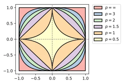
Figure 2.1: ℓp norm ballsBk·k_p in a two-dimensional space, for several values of

p. The legend matches the outside-to-inside ordering of the contours. Forp < 1, ℓp are not proper norms; as p → 0the limit vectors have exactly one nonzero

coordinate.

Often called theℓ0norm by abuse of language, this function is not a metric norm, but, if the domain is bounded, it is a limit ofℓpnorms, namely k·k0= limp→0k·kpp.

The ℓ0 function is discontinuous and non-convex, and optimization problems involving it are typically NP-hard. However, otherp-norms can be used toinduce

sparsitywhile leading to simpler optimization problems. The most commonly

used such surrogate is theℓ1norm,kxk1 =Íi|xi|. It is convex and continuous, and

minimizing or constraining its value yields sparse solutions.

To see why, we introduce theunit ballof anℓppenalty function

B_k·k

p = {x ∈R

d _{: kxk}

p ≤ 1}.

Figure2.1illustrates unit balls for several interesting norms. In particular, it can be seen thatB_k·k1 is a polytope with vertices{±ei : i∈ndo}. The fundamental

theorem of linear programming states that the minimum of a linear function over a polytope (including B_k·k

1) is always attained at a vertex (Dantzig et al., 1955, Theorem 6); similarly, the minimum of a quadratic function over a polytope is

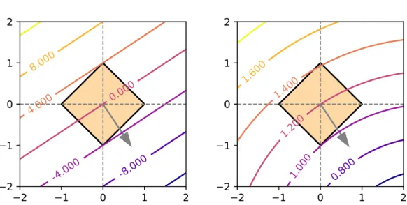
2 1 0 1 2 2 1 0 1 2 -8.000 -4.000 0.000 4.000 8.000 2 1 0 1 2 2 1 0 1 2 0.800 1.000 1.200 1.400 1.600

Figure 2.2: When optimizing a linear function (left) or a quadratic function (right) over theℓ1 ball, solutions are likely sparse.

likely (but not always) attained at a vertex. Both phenomena are illustrated in Figure 2.2. Since euclidean projections are quadratic minimizations, it follows that PB_{k · k}

1 has sparse solutions. We further note that the d-simplex is a face of thed-dimensionalℓ1ball, suggesting that similar optimization problems over the simplex also result in sparse solutions; we later prove a more general result about what probability mappings are sparsity-inducing in Proposition3.1.

Vertex sparsityis a notion of simplicity for points in a polytopeP ₌convV.

Recall that anyx ∈P can be represented as a convex combination of its vertices:

∀x ∈P ∃α ∈ △|V|, x=

Õ

v∈V

αvv. (2.11)

In some cases, for instance if all vertices are strictly positive vectors,i. e.,v ≻ 0,

P may even contain no points with sparsecoordinates. Yet, by shifting to the repre-sentation in Equation2.11, we find that some points can be compactly represented as sparseconvex combinationsinvolving only a few vertices,i. e.,kαk₀ ≪ |V|. This

are sparse vectors, then vertex sparsity results in coordinate sparsity as well.²

Group sparsity. In some cases, the coordinates of a vectorx ∈ _Rdhave some

known meaning, and we might want several coordinates to either all be zero or all be nonzero. We may organize the indices into groupsG_i ⊂ ndok_i

=1.Thegroup lasso

penalty (Yuan and Lin,2006) is defined as

RGL(x)=

k Õ

i=1

xG_i2.

If k = d and each coordinate is in a separate group,i. e.,Gi = {i}, then the group

lasso reverts to theℓ1penalty discussed above. While originally proposed for non-overlapping groups, the group lasso has been extended to unions and intersections of overlapping groups (Jacob et al.,2009;Jenatton et al.,2011).

Fusing values. Parsimony can go beyond zeroing out coordinates, vertices or

groups. We may also encourage simplicity in a vector by clustering (fusing) together its values. An important instance of this is the fused lasso, used to smoothen or denoise a 1-d sequence (represented as a vector x by encouraging adjacent

coefficients to be exactly equal. This can be done by penalizing the absolute value of their difference (Tibshirani et al.,2005)

RFL(x)=

d−1

Õ i=1

|xi+1−xi|. (2.12)

More generally, given a graph over thedindices, weighted by a matrixW ∈_Rd×d,

we may define ageneralizedfused lasso penalty (Tibshirani and Taylor,2011)

RGFL(x)=

Õ i<_j

wij|xi−xj|. (2.13)

Unlike the 1-d version, for which efficient exact algorithms exist, the general formulation is more challenging.

In some cases, the actual ordering of the coefficients doesn’t matter, but we might still desire a parsimonious vector with only a few distinct values. The OS-CARregularizer (Bondell and Reich,2008) achieves this effect without incurring the high computational cost of the generalized fused lasso.

ROSC = λ1kxk+λ2

Õ i<_j

max(|xi|,|xj|). (2.14)

Generalized penalties. There has been a lot of interest in the study of more

generalized structured norms and penalties. We briefly list some directions, useful not only in hand-crafting better suited penalties for a task as hand, but also for their analysis which can lead to insights into the penalties discussed above.

Theordered weightedℓ1(OWL)norm (Zeng and Figueiredo,2015) is

ROWL(x)=

Õ i

wi|x↓_i|,

wherex↓_i denotes theith largest element ofx. With the weight defined aswi = 1,

OWL is equal to theℓ1norm; whenw1 = 1and wi = 0fori > 1it amounts toℓ∞,

and forwi = λ1+λ2(d−i), OWL becomes the OSCAR regularizer in Equation2.14.

Another perspective is given throughatomic norms(Chandrasekaran et al.,

2012). A set ofatomsAk ⊂ _Rd induces, under some assumptions, the norm

kxkA =inf{t ≥ 0 :x ∈tconvA}.

Atomic norms induce representations as sparse affine combinations of atoms. ForA ₌ {±ei : i ∈ ndo},k·kA = k·k1; for A = {−1,1}d,k·kA = k·k∞. An atomic

CHAPTER 3

STRUCTURED SPARSITY FOR ATTENTION MECHANISMS

In this chapter, we focus on neural attention mechanisms: latent selector mod-ules which decide on what part of the input a network should focus. We empower these mechanisms withsparsity, in particular structured sparsity, by proposing a regularization-based framework for attention. We recover within this framework the popular attention mechanisms known as softmax and sparsemax, leading to new insights into them.

Building on well-studied structured penalties, we develop new and more inter-pretable attention mechanisms, that focus on entire segments or groups of an input. We derive efficient algorithms to compute the forward and backward passes of our attention mechanisms, enabling their use within neural networks. Our attention mechanisms are efficient and interpretable drop-in replacements for softmax. For certain applications, the structured priors incorporated by our methods can lead to superior results.

This chapter is based onNiculae and Blondel(2017).

3.1 Motivating Structured Sparsity For Attention

Modern neural network architectures are commonly augmented with an attention mechanism, which tells the network where to look within the input in order to make the next prediction. Attention-augmented architectures have been successfully applied to machine translation (Bahdanau et al.,2015;Luong et al.,2015), speech recognition (Chorowski et al.,2015), image caption generation (Xu et al.,2015), textual entailment (Rocktäschel et al., 2016; Martins and Astudillo, 2016), and

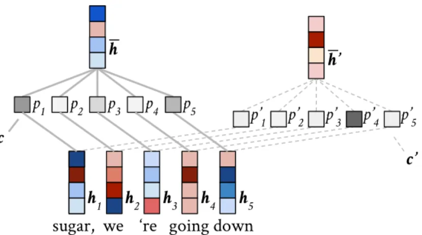
sugar, we ‘re going down h₁ h₂ h₃ h₄ h₅ p₁ p₂ p₃ p₄ p₅ p’₁ p’₂ p’₃ p’₄ p’₅ c c’ h h’

Figure 3.1: A generic attention mechanism computes a representative vector_h¯_{as a} context-dependent weighted average of a sequence of vectors(hi), by inducing a

probability distribution over them,i. e.,_h¯₌ Í_{i pihi. For different contextscandc}′_,

the distributionspandp′_{may be wildly different.}

sentence summarization (Rush et al.,2015), to name but a few examples.

Attention is used to select, out of a variable-length list of vectors representing items (e. g., words), a single representative vector, given some context (Figure3.1). A popular and illustrative application is in sequence to sequence(seq2seq) neural machine translation, where a recurrent neural net (RNN)encoderfirst transforms each of thedsource words into a vectorhi ∈Rk, wherei ∈ [d]. Then, thedecoder

incrementally predicts target words, using a traditional multi-class classifier (with one class per known word in the target language). The input to this classifier, however, is context-sensitive: at each time stept, the input combines the current

decoder hidden state contextc(t−1)_{, and theattentionvectorwhich approximates the}

most relevant source word, given the current context:

¯ h(t) = d Õ i=1 pihi where pi = pi(hi,c(t−1)).

In an idealized simplified case, when translating one word, we would need to look only at the unique relevant source word j, so we would like the probabili-tiespto concentrate on the one-hot vectorej. Relaxing this discrete selection to

a continuous probability allows the model to hedge its bets and capture uncer-tainty. Importantly, continuous attention also allows such models to be trained via backpropagation, since the probabilitiespare differentiable.

Estimating this latent relevance probability is not trivial. The key insight behind attention mechanisms is to parametrize this probability using two components:

1. a regression-likescorermodule, generating a relevance score for each word

hi relative to some contextc:

(hi,c) → θi ∈R

2. a normalizingprobabilitymappingΠ: θ → pfrom scores into probabilities.

By far, the most common such mapping is the softmax:

pi =softmax(θ)i = Í_dexpθi

j=1expθj

These two components are present in all newly-proposed types of attention mech-anisms: self-attention (Lin et al.,2017), key-value attention (Daniluk et al.,2017), pointer networks (Vinyals et al.,2015), etc.

Alongside empirical successes, neural attention—while not necessarily cor-related with human attention—is increasingly crucial in bringing more

inter-pretabilityto neural networks by helping explain how individual input elements

contribute to the model’s decisions. It is common to inspect and report atten-tion distribuatten-tion as heatmap plots; forseq2seqmodels, such plots often look like Figure3.2a.

A notable property of softmax is that its outputs arealways dense: there are no scoresθ such thatsoftmax(θ)k = 0for somek. For simplicity, human operators

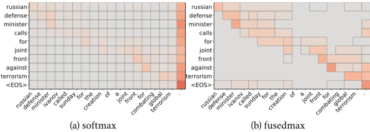
russiandefenseministerivanovcalledsundayfor thecreation of ajointfront for_combatingglobal_terrorism . russian defense minister calls for joint front against terrorism <EOS> softmax (a) softmax

russiandefenseministerivanovcalledsundayfor thecreation of ajointfront for_combatingglobal_terrorism . russian defense minister calls for joint front against terrorism <EOS> fusedmax (b) fusedmax

Figure 3.2: Traditionally, attention mechanisms use softmax for mapping scores to probabilities, yielding dense, not very interpretable results (3.2a). Within our frame-work, we can derive attention mechanisms that yield sparse, clustered probabilities, aiding interpretability (3.2b).

will focus only on the first few highest-weighted items, but because the attention weights are never zero, all elements in the input always make at least a small contribution to the decision. This leads to a disconnect between ourperceptionof the model and the actual model.

To overcome this limitation,Martins and Astudillo(2016) recently proposed

sparsemax, using the Euclidean projection onto the simplex as a sparse alternative to softmax. But, as we have seen in Section2.3, the principle of parsimony, stating that simple explanations should be preferred over complex ones, goes well beyond such

coordinate-levelsparsity: depending on the application, it may be useful to consider selection of entire groups, of rectangles and convex shapes, or of equally-weighted clusters. Such properties, thoroughly studied in the field ofstructured sparsity, can lead to better interpretability, as well as to more adequatestructural prior knowledge assumed by the model.

(1, 0, 0) (0, 1, 0) (0, 0, 1) 0.200 0.400 0.600 0.800

Figure 3.3: Finding the maximum coordinate of a vector (here, θ = [.5,1,0]) is

equivalent to maximizing a linear function over the simplex. As the simplex is non-empty, a solution is always achieved at a vertex.

3.2 Regularized max Operators

In this section, we shed light on the intimate connection between themaxfunction and anarg max-like mapping fromRd toΔd. Using a smoothing technique from convex analysis, we extend this intuition to an entire family of regularizedmax operators and their probability mappings, recovering well-known expressions.

Reformulatingmaxas an optimization problem. The maximum operator is

a function fromRd toRand can be defined by

max(θ) ≔ max

i∈[d] θi = sup_p∈Δd

p⊤θ. (3.1)

The equality on the right-hand is an essential insight, and it stems from the fact that the supremum of a linear form over the simplex is always achieved at a vertex. This is a direct consequence of the fundamental theorem of linear programming (Dantzig et al.,1955, Theorem 6), illustrated in Figure3.3. Moreover, by Danskin’s theorem (Danskin,1966), any optimalp⋆_{is a subgradient of the supremum. More}

strongly, we have

∂max_(θ)= conv_{ei⋆: i⋆∈arg max i∈[d]

θi}. (3.2)

We can see∂max_(θ)as a mapping_{Π: R}d → Δd. When there are no ties,∂max concentrates all probability mass onto the highest-scoring item: Π(θ)₌ ei⋆. This

mapping is, however, ill-behaved in crucial ways: it is multi-valued whenever there are ties, it is discontinuous, and it is piecewise constant wherever continuous (since small enough changes to θdo not change the maximum, in general). Therefore, ∂maxis not amenable to optimization by gradient descent, and thus unsuitable for direct use in neural network hidden layers.

A regularized max operator and its gradient mapping. These shortcomings

encourage us to consider a regularization of the maximum operator. Inspired by the seminal work ofNesterov(2005), we apply a smoothing technique. The conjugate ofmax(θ)is max∗_(p) =Id△d =     0, ifp ∈ △d ∞, otherwise. (3.3)

To prove this, we note thatId∗

△d =max (Boyd and Vandenberghe,2004, Example

3.24), and that, since△dis closed and convex,Id∗∗

△d =Id△d. Taking the conjugate of

both sides leads to the desired result. We proceed to add regularization tomax∗ max∗ Ω(p)≔ Id△d +γΩ(p)=     γΩ(p), if p∈ △d ∞, otherwise. (3.4)

where we assume thatΩ: Rd →_Ris β-strongly convexw.r.t. some norm k · kand

take the conjugate once again maxΩ(p)≔ max∗∗ Ω(θ)= sup p∈Rd p⊤θ−max∗_Ω(p)= sup p∈△d p⊤θ−γΩ(p) (3.5)

Our main proposal is a mappingΠΩ: Rd → △d, defined as theargumentthat achieves this supremum.

ΠΩ(θ) ≔ arg max p∈△d

p⊤θ−γΩ(p)= ∇maxΩ(θ) (3.6)

The right-hand side follow from i)maxΩ(θ)=(p⋆)⊤θ−max∗_Ω(p⋆) ⇔ p⋆∈∂maxΩ(θ)

and ii) ∂maxΩ_{(θ) = {∇}maxΩ_(θ)}, since (3.5) has a unique solution. Therefore, _ΠΩ is agradient mapping. We illustratemaxΩ and ΠΩ for various choices ofΩ in Figure3.4(2-d), in Figure3.5on the 3-dimensional simplex, and in Figure3.6in a 3-d cross section.

Importance of strong convexity. Our β-strong convexity assumption on Ω plays a crucial role and should not be underestimated. Recall that a function

f: Rd →_Ris β-strongly convex w.r.t. a normk · kif and only if its conjugate f∗ is

1

β-smooth w.r.t. the dual norm k · k∗ (Zălinescu,2002, Corollary 3.5.11) (Kakade et al.,2012, Theorem 3). This is sufficient to ensure thatmaxΩis 1

γ β-smooth, or, in

other words, that it is differentiable everywhere and its gradient,ΠΩ, is_{γ β}1-Lipschitz continuous w.r.t.k · k∗.

Training by backpropagation. In order to useΠΩin a neural network trained by backpropagation, two problems must be addressed for any regularizerΩ. The first is the forward computation: how to evaluateΠΩ(θ), i.e., how to solve the optimization problem in (3.5). The second is thebackward computation: how

4

2

0

2

4

0

1

2

3

4

_max

max ([

,0])+ const

softmax

sparsemax

sq-pnorm-max

fusedmax

4

2

0

2

4

0.0

0.2

0.4

0.6

0.8

1.0

([

,0])

= max ([

,0])

Figure 3.4: The proposedmaxΩ(θ)operator up to a constant (left) and theΠΩ(θ) mapping (right), illustrated forθ =[t,0]. In this case,maxΩ(θ)is hinge-shaped and ΠΩ(θ)is sigmoid-shaped. Our framework recoverssoftmaxandsparsemax.

our key contributions, presented in Section3.4, is to show how to solve these two problems for general differentiableΩ, as well as for two structured regularizers: fused lasso and OSCAR.

3.3 Recovering Known Mappings and Characterizing Sparsity

Before deriving new attention mechanisms using our framework, we first show how our framework recovers softmax and sparsemax by careful choice ofΩ.

Softmax. We chooseΩ(p) = Íd_i=1pilogpi, the negative Shannon entropy. The

conjugate of the negative entropy restricted to the simplex is thelog sum exp(Boyd and Vandenberghe, 2004, Example 3.25). Moreover, if f(x) = γg(x) for γ > 0,

then f∗_(y)

= γg∗(y/γ). We therefore get a closed-form expression: maxΩ(θ) = γlogÍd_i=1exp(θi/γ).Since the negative entropy is1-strongly convex w.r.t.k · k1over

with temperature parameterγ, by taking the gradient ofmaxΩ(θ), ΠΩ(θ)= exp (θ/γ) Íd i=1exp(θi/γ) , (softmax)

whereexp(θ/γ)is evaluated element-wise. Note that some authors also callmaxΩa

“soft max.” AlthoughΠΩis really a softarg max, we opt to follow the more popular terminology. Whenθ = [t,0], it can be checked thatmaxΩ(θ)reduces to the softplus

(Dugas et al.,2001) andΠΩ(x)1to a sigmoid Figure3.4.

Sparsemax. We chooseΩ(p)= 1₂ kpk22, also known as Moreau-Yosida regulariza-tion in proximal operator theory (Nesterov,2005;Parikh and Boyd,2014). Since

1 2k·k

2

2is1-strongly convex w.r.t.k·k2, we get thatmaxΩis 1_γ-smooth w.r.t.k·k2. In addition, it is easy to verify that

ΠΩ(θ)=P△d(θ/γ)=arg min

p∈△d

kp−θ/γk2. (sparsemax)

This mapping was introduced in an ad-hoc manner byMartins and Astudillo(2016) and was named sparsemax, due to the fact that it is a sparse alternative to softmax. The Euclidean projection onto the simplex,P△d, enjoys exactO(d)algorithms (Held et al.,1974;Brucker,1984;Condat,2016). Following (Martins and Astudillo,2016), the Jacobian ofΠΩis J_ΠΩ(θ)= 1 γJP△d(θ/γ)= 1 γ diag(s) −ss ⊤_/ksk 1 , (3.7)

wheres ∈ {0,1}d indicates the nonzero elements ofΠΩ(θ). SinceΠΩ is Lipschitz continuous, by Rademacher’s theoremΠΩis differentiable almost everywhere. For points whereΠΩis not differentiable (i. e.,maxΩis not twice differentiable), we can take an arbitrary matrix in the set of Clarke’s generalized Jacobians (Clarke,1990), the convex hull of Jacobians of the form lim

θt→θ

A condition for sparsity. The closed form ofsoftmaxmakes it obvious that the probabilities it produces can never be exactly zero, sinceexpis strictly positive. Moreover, quadratic problems over the simplex yield sparse solutions (Figure2.2), justifyingsparsemax. However, for an arbitrary convexΩ, it is nota prioriobvious whetherΠΩwill be sparse or dense. The following proposition provides a necessary and sufficient condition for sparsity.

Proposition 3.1 Let Ω : △d → _R be a strictlyconvex function. The mapping ΠΩ

covers thefull simplex, i. e.,ΠΩ(Rd)= △d, if and only if∂Ω(p),œ for anyp∈ △d.

Proof is given in AppendixA.1. Functions whose gradient “explodes” in the bound-ary of their domain (hence failing to meet the condition in Proposition3.1) are called “essentially smooth” (Rockafellar,1970); an example is the negative Shannon entropy. For such functions,ΠΩ maps only to the relative interior of △d, never attaining boundary points (Wainwright and Jordan, 2008). This prevents these functions from generating sparse attention mappings.

3.4 Algorithms for General Differentiable Regularizers

Before tackling more structured regularizers, we address in this section the case of general differentiable regularizerΩ. BecauseΠΩ(θ)involves maximizing (3.5), a concave function over the simplex, its solution can be found using off-the-shelf projected gradient solvers. Therefore, the main challenge is how to compute the Jacobian ofΠΩ. This is what we address in the next proposition.

Assume thatΩ istwicedifferentiableover△d and thatΠΩ(θ)=arg maxp∈△d p⊤θ−

γΩ(p) = p⋆ has been computed. Then the Jacobian of ΠΩ at θ, denoted JΠΩ, can be obtained bysolving the system

(I + A(B−I))JΠΩ = A, (3.8)

where wedefined the shorthands A ≔ J_P

△d(p

⋆

−γ∇Ω(p⋆)₊θ) and B≔ γHΩ(p⋆).

The proof is given in AppendixA.2. Unlike recent work tackling argmin differen-tiation through matrix differential calculus on the Karush–Kuhn–Tucker (KKT) conditions (Amos and Kolter,2017), our proof technique relies on differentiating the fixed point iterationp∗ =P△d(p

⋆

− ∇Ω(p⋆)₊θ).

Efficient computation. When training networks by backpropagation, the

Jaco-bian is only accessed via products with vectors, to obtaindθ ≔ JΠΩ

⊤_d

p. Therefore, we may directly solve(I + A(B− I)) dθ = Adp. As a sparsemax Jacobian (Equa-tion3.7),Ais row-and column-sparse, and uniquely defined by its sparsity pattern.

By splitting the system into equations corresponding to zero and nonzero rows of A, we obtain that the solutiond_θ must have the same sparsity pattern as the

row-sparsity ofA, therefore we only need to solve a subset of the system. From the

fixed-point iterationp⋆= P△d(p

⋆

− ∇Ω(p⋆)₊θ), it follows that the row-sparsity of Ais the same as the sparsity of the forward pass solution p⋆. The Jacobian-vector

product can thus be computed inO(nnz(p⋆)3).

Example: squaredp-norms. As a useful example of a differentiable function

over the simplex, we consider squared p-norms: Ω(p) = 12 kpk 2 p = Íd_i=1p p i 2/p , where p ∈ △d and p ∈ (1,2]. For this choice of p, it is known that the squared