Simultaneous Bayesian clustering and feature selection through student’s t mixtures model

(1)

Simultaneous Bayesian Clustering and Feature

Selection Through Student’s t Mixtures Model

Jianyong Sun, Aimin Zhou, Member, IEEE, Simeon Keates, and Shengbin Liao

Abstract— In this paper, we proposed a generative model for feature selection under the unsupervised learning context. The model assumes that data are independently and identically sampled from a finite mixture of Student’s t distributions, which can reduce the sensitiveness to outliers. Latent random variables that represent the features’ salience are included in the model for the indication of the relevance of features. As a result, the model is expected to simultaneously realize clustering, feature selection, and outlier detection. Inference is carried out by a tree-structured variational Bayes algorithm. Full Bayesian treatment is adopted in the model to realize automatic model selection. Controlled experimental studies showed that the developed model is capable of modeling the data set with outliers accurately. Further-more, experiment results showed that the developed algorithm compares favorably against existing unsupervised probability model-based Bayesian feature selection algorithms on artificial and real data sets. Moreover, the application of the developed algorithm on real leukemia gene expression data indicated that it is able to identify the discriminating genes successfully.

Index Terms— Bayesian inference, feature selection, robust clustering, tree-structured variational Bayes (VB).

I. INTRODUCTION

C

OMPETITIVE performances of clustering algorithms cannot be expected on high-dimensional data sets due to the curse of dimensionality and the impact of redun-dancy and noise. Fortunately, the intrinsic dimensionality of a high-dimensional data set is usually much less than original feature space [1]–[3]. The performance of a learning algorithm could be improved significantly if a subset of features or a combination of features is properly selected [4]. Feature selection is to select a subset of most informative features (or attributes, variables) rather than selecting a combination TheworkofJ.SunwassupportedbytheNationalScienceFoundationof China under Grant 61573279, Grant 61573326, and Grant 11301494. The work of A.Zhou was supported by NSFC under Grant 61673180. The work of S.Liao was supported by the Key Science and Technology Project of Wuhan under Grant 2014010202010108. (Corresponding authors: Jianyong Sun;AiminZhou.)

J. Sun is with the School of Mathematics and Statistics, Xi’an Jiaotong University, Xi’an 710049, China, and also with the School of Computer Science, University of Essex, Colchester, CO4 3SQ, U.K. (e-mail: [email protected]).

A. Zhou is with the Shanghai Key Laboratory of Multidimensional Information Processing, and also with the Department of Computer Science and Technology, East China Normal University, Shanghai 200062, China (e-mail: [email protected]).

S. Keates is with the Faculty of Engineering and Science, University of Greenwich, Kent, ME4 4TB, U.K.

S. Liao is with the National Engineering Research Centre for E-Learning, Huazhong Normal University, Wuhan 430079, China.

of features (which is usually referred to as feature extraction), such as in principal component analysis and independent component analysis.

Existing feature selection algorithm can be categorized as supervised feature selection (on data with full class labels) [5]–[9], unsupervised feature selection (on data without class labels) [10]–[15], and semisupervised feature selection (on data with partial labels) [14], [16], [17]. Feature selection in unsupervised context is considered to be more difficult than the other two cases, since there is no target information available for training. The selected informative features must greatly preserve the distribution and the manifold structure of the data space. In this paper, we focused on unsupervised feature selection.

Various feature selection methods for unsupervised learning have been developed, which can be categorized according to different feature selection criteria. Criteria scores, such as Laplacian score [18], eigenvalue sensitive criteria [19], information entropy [20], and correlation [21], have been proposed. In [22], consistency-based feature selection methods were proposed and evaluated. To preserve pairwise similarity along data samples in the original data space, a similarity preserving feature selection framework is proposed in [11]. Local learning-based feature selection methods [13] have been extensively studied recently. For examples, in [23] and [24], subspace learning based on nonnegative matrix factorization is developed, where the loading matrix is penalized by L2and/or

L1 norms. Moreover, L2, L1, and L2,1-norms have been widely applied in various feature selection methods, such as in [25]–[27]. In [17], a global and local structure preservation framework that integrates global pairwise sample similarity and local geometric data structure is proposed for feature selection. In [15] and [28]–[31], spectral learning aiming to preserve the underlying manifold structure is applied for selecting proper features. In [32], embedding learning and sparse regression are jointly applied to perform feature selection. A discrimination analysis based on a property of Fourier transform of the data density distribution is applied for feature selection via optic diffraction principle [10]. A theo-retically optimal criterion, namely, the discriminative optimal criterion, has been developed for feature selection in [33].

Apart from these mentioned algorithms, clustering (which aims to discover data structure) can also be used as a criterion. Intuitively, informative feature subsets that greatly preserve the sample data distribution should vary at different clusters. In the wrapper method proposed in [4], a clustering algorithm is used to evaluate the candidate feature subsets. The performance of the wrapper method highly depends on the employed

(2)

clustering algorithms. Alternatively, clustering and feature selection are embedded together with a proper objective function. Subset features can be obtained by optimizing the objective function. It is well acknowledged that the choosing of feature subsets and the clustering estimation (including the cluster statistics and the optimal number of components) are highly dependent problem [34]. This clearly suggests that the two problems should be considered simultaneously.

Most of clustering-based feature selection methods were developed on finite Gaussian mixtures. Carbonetto et al. [35] proposed a Bayesian shrinkage approach where shrinkage hyperpriors are placed over the component means. The shrink-age hyperpriors can lead to automatic feature selection. Pan et al. [36] proposed a penalized likelihood approach where a L1 penalty is imposed on the cluster means. The proposed approach can automatically realize feature selection through thresholding and model selection through the BIC criterion. Law et al. [37] defined the saliency of feature as a probability, which is to quantify whether the data distribu-tion with respect to the saliency features can be sufficiently represented. They proposed to fit the Gaussian mixture model to the sample data distribution using the EM algorithm, while the MML criterion is employed for model selection. Moreover, a Bayesian treatment to the finite Gaussian mixture model that benefits from automatic model selection was proposed in [34]. Li et al. [38] improved their work by utilizing “localized” feature saliency to address the local intrinsic property of data.

Outliers or scattered objects exist elsewhere in real data sets. As well known, Gaussian mixture models are not able to deal with outliers properly. The outliers, if exist, should seriously deteriorate the performances of Gaussian-based clustering algorithms. Moreover, the presence of outliers could also lead to selecting a false model complexity, and make the optimal selection of a subset of informative features get much more difficult. Therefore, previous clustering-based feature selection methods cannot be expected to perform well on data with outliers. It is thus indispensable to propose a principled approach to realize the selection of the most informative features and the improvement on the clustering performance, while eliminating the bad effect of outlying data. This motives us to propose a finite mixture model that is able to deal with outliers; and to develop a Bayesian inference algorithm that can carry out unsupervised clustering, feature selection, and outlier detection simultaneously.

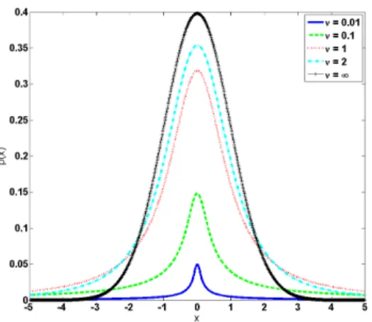
Specifically, in this paper, we propose a hierarchical latent variable model to address the three tasks. First of all, it has been a common practice to adopt heavy-tailed distributions for handling outlier data in the literature. The Student’s t distribution is such a heavy-tail distribution, and has been widely used [39], [40]. In our model, we adopt a finite mixture of Student’s t distributions as the backbone. Fig. 1 shows the difference between a Student’s t distribution and a Gaussian distribution with the same mean and variance, but with different parameters (ν, also called the degree of freedom). There are other heavy-tail distribution is available, such as the Laplace distribution and the Pearson type-VII distribution [40], which can also be adopted for handling outliers. Note that the

Fig. 1. Demonstration of the Student t-distribution with different parameters ν = 0.01,0.1,1,2,∞. Note that the Student t-distribution becomes the Gaussian distribution in caseν= ∞.

Student’s t is a scalar mixture of Gaussians. This property makes the Student’s t distribution convenient for inference, and hence popular for outlier detection.

Second, regarding feature selection, we propose to use a localized feature saliency similar to the approach developed in [38]. The feature saliency characterizes the importance of the feature and can be used as criterion for the selection of the most informative features. Localization of the feature saliency addresses the cluster effect on relevant feature subsets. Finally, to carry out model selection, we adopt a full Bayesian treatment to the model, where proper prior distributions are assumed for the parameters, including the number of clusters, the mixing proportions, and the parameters of the cluster com-ponents. To carry out inference, we resort to a tree-structured variational Bayesian (VB), since the likelihood function of the training data with respect to the proposed model is not tractable.

In the rest of this paper, Section II presents the proposed latent variable model. The inference is presented in Section III-A–III-F, in which the tree-structured VB algorithm is described. Moreover, the interpretation of the model is described in Section III-G. The experimental study is presented in Section IV. In this paper, controlled experiments were first carried out to justify the out performance of the developed models over the model using Gaussian distributions on syn-thetic data sets and another state-of-the-art feature selection algorithms. Then, the developed algorithm was compared with them on some real data sets. Section V concludes this paper.

II. MODEL

In this section, we present the proposed hierarchical latent variable model step by step starting from the introduction of saliency features to variables that are modeled to follow the mixture of Student’s t. To make the description clear, Table I shows the notations used.

Suppose that a vector of random variable Y = (Y1, . . . ,Yd)∈Rd, where d is the dimensionality of the input data, and denote Y as theth feature. In the sequel, we use

y to represent the realization of Y . To represent if a feature

is relevant or not, we use a vector of random binary variable = (φ1, . . . , φd). That is, if φ = 1, we say that the th feature is relevant, and 0 otherwise.

(3)

TABLE I

NOTATIONSUSED INMODELING

To handle outliers, heavy-tailed probability distributions, such as Student’s t distribution [41] or Pearson type-VII distribution [40] can be used. Taking the features’ relevancy into consideration in the Student’s t distribution, we result in the following model:

p(y|;)=

d

=1

[St(y|θ)]φ[St(y|γ)]1−φ (1) where St represents the Student’s t distribution.

To realize clustering, a finite mixture of p(y|;)can be applied. That is p(y|;)= K j=1 πjp(y|, j)

where = {j} and j = {θj, γj,1 ≤ ≤ d} are the parameters of the cluster components. To this end, we can introduce a discrete latent variable z to specify which cluster that the data belongs to, and a Bernoulli prior over with parameter β to characterize the importance of features. To account for the case that in different clusters, features might have different relevance, we propose to impose thatdepends on the latent variable z. As a result, βj,1 ≤ j ≤ K,1 ≤ ≤d are the parameters associated with the Bernoulli prior

overdepending on z, which are called feature saliency [37]. Mathematically, the model can be written hierarchically for a set of training data yn,1≤n≤ N as follows:

p(yn|n,zn) = K j=1 _d =1 [St(yn|θj)]φn[St(yn|γj)]1−φn δzn,j p(n|zn, β) = K j=1 _d =1 βφn j (1−βj) 1−φn δzn,j

wherenand znare latent variables associated with each data point yn, andδzn,j is the Kronecker delta function. Note that

a similar idea has been implemented in [38] which is termed

as “localized feature saliency.” The difference between their work and our work is that we impose dependencies between nto znand yn, while in [38], the dependence is implemented by introducing different feature saliency variables in different classes (which results in φn j for 1 ≤ j ≤ K rather than justφn as in our implementation). Note that the Student’s t distribution can be written as a convolution of a Gaussian and a gamma distribution as follows:

St(y|θ)= N(y|μ, σu)G u|ν 2, ν 2 du

whereσ is the precision (inverse variance) andθ=(μ, σ, ν) is the parameters, and

G(x|a,b)=baxa−1exp(−bx)

(a) .

If we introduce un=(un1, . . . ,und)and vn=(vn1, . . . , vnd) as latent variables for the Student’s t components with and without relevant features, respectively, we can obtain a distribution of p(yn|n,un,vn,zn)as follows: p(yn|n,un,vn,zn) = K j=1 ⎡ ⎣d =1 N(yn|μj,unσj)φn ×N(yn|χj, vnτj)1−φn ⎤ ⎦ δzn,j .

The hierarchical latent variable model is completed by introducing conjugate prior over zn,un and vn as follows:

p(un|zn)= K j=1 _d =1 G un νj 2 , νj 2 δzn,j p(vn|zn)= K j=1 _d =1 G vn γj 2 , γj 2 δzn,j p(zn)= K j=1 πδzn,j j .

To realize model selection, i.e., selecting the optimal number of components, we adopt the full Bayesian treatment, which means that we need to specify conjugate priors for the parame-ters (i.e.,). The conjugate priors associated with the model parameters are as follows:

p(β)= K j=1 d =1 B(βj|κ1, κ2) p(σ)= j p(σj)= j Gσjη0 2, ω0 2 p(μ)= j p(μj)= j N(μj|m0, λ0) p(χ)= j p(χj)= j N(χj|m0, λ0) p(τ)= j p(τj)= j Gτjη0 2 , ω0 2 p(π)=D(π|α0) (2)

(4)

Fig. 2. Plate diagram of the proposed hierarchical graphical model.

whereB(x|a,b)represents the Beta density function

B(x|a,b)= x

a−1₍₁₋_x₎b−1

B(a,b)

and B(a,b) is the beta function, G(x|a,b) is the gamma distribution, and D(π|α0)= K k=1αk0 K k₌1 α0 k K k=1 παk0−1 k

is the Dirichlet distribution. The parameters in the priors, including κ1, κ2, η0, ω0,m0, λ0, and α0 are considered as hyperparameters. Note that in the priors, we assume the same hyperparameters for σj andτj and for μj andχj, respectively. The resultant model can be depicted using the plate diagram shown in Fig. 2. In a rectangle of the plate diagram, the bold typeset indicates the dimensions of the circled variables. For example, Kd means that there are K×d

variables of νj,1 ≤ j ≤ K,1 ≤ ≤ N . The arrows in the diagram indicate the variable dependencies, e.g., the arrow pointing to U from Z means that U depends on Z .

In the following, we use n, , and j to denote the index of the data point, the features, and the mixing component. We omit the typeset of parameters in the formula.

In the proposed model, bear in mind that the joint probability distribution is written as

p(yn,un,vn, n,zn|)

where= {μ, σ, χ, τ, π, β, ν, γ}and it can be factorized as

p(yn|n,un,vn,zn)p(n|zn)p(un|zn)p(vn|zn)p(zn) and are fully factorized over the dimensions. In the sequel, we denote the latent variables as hn = {un,vn,zn, n,1 ≤

n ≤ N}. According to the model, the complete likelihood of a data yn can be written as follows:

L_C(yn,hn, )= p(yn,hn|)p() (3) where p() = p(μ)p(σ)p(β)p(π)p(χ)p(τ). Note that we

assume the same hyperparameters of the prior distributions corresponding to the parameters with respect to all the com-ponents. We do not assume any priors forνandγ, since there are no conjugate priors.

TABLE II

NOTATIONSUSED IN THEINFERENCE

III. INFERENCE

In this section, we first define some notations as listed in Table II. These notations will be used in the inference. A brief introduction to the VB method is given, while the detailed inference follows. The algorithm is then summarized and interpreted.

A. Brief Introduction to VB

The integration of p(yn,un,vn, n,zn|)p() over the latent variables and the parameters is not tractable. Therefore, exact inference is impossible. We adopt the VB algorithm for model inference [42]. To apply the VB algorithm, the evidence, obtained by integrating out the latent variables (denoted by H) and the parameters (denoted by ) given a model structure M, is approximated by introducing an auxiliary distribution q. The lower bound to the evidence is as follows: log p(X|M)≥ Hq(H, )log p(Y,H, |M) q(H, ) dHd = log p(Y,H, |M)q− log q(H, )q F(q(H),q(),Y,M) (4)

where p(Y,H, |M) is the complete data likelihood and

q(H, ) =q(H)q() is the auxiliary posterior distribution,

F(q(H),q(),Y,M)is called the free energy. In the equa-tions, we use·q to denote the expectation with respect to q. It is obvious that maximizing the evidence is equivalent to maximizing the free energyF.

To maximize the free energy, we apply coordinate ascent search as adopted in [43]. Applying the coordinate ascent search, the auxiliary distributions of latent variable

H and parameters are optimized alternatively as follows: q(t+1)(H)=arg max q(H)F(q(H),q t_(), Y,M) q(t+1)() =arg max q()F(q t+1₍_H_),_q_(),_Y_,_M_).

(5)

B. Tree-Like Factorization of the Random Variables

We propose a tree-like factorization over the latent variables for the auxiliary posteriors (i.e., q(H)). Tree-like structural factorization in VB has been shown to be superior over the full factorization scheme [44], [45]. The factorization can be summarized as follows: q(hn, π,{βj},{μj, σj},{χj, τj}) =q(un|zn)q(n|zn)q(vn|zn)q(zn) ×q(π)q({βj})q {μj, σj} q{χj, τj} . The tree-like factorization is reflected on the dependences between un,vn, n, and zn. Specifically, due to the full factorization over the features and the conjugate prior we used, it can be seen that

q(hn, ) =q(zn) n q(vn|zn)q(un|zn)q(φn|zn) ×q(π) j q(χj)q(τj)q(βj)q(μj)q(σj). The auxiliary posteriors of the latent variables and the parameters can be obtained by maximizing the free energy associated with the proposed model

F = log LC(yn,hn, )q− log q(hn)q (5) where ·q is the expectation with respect to the auxiliary posterior q.

C. Auxiliary Posteriors of the Latent Variables

The free energy associated with the auxiliary posterior

q(un|zn)can be read as follows:

F= log[p(yn,hn)] −log q(un|zn)q.

According to the KKT condition, and using the Lagrange multiplier, we obtain (see the Appendix for details)

q(unzn)∝ d

=1

explog[p(yn|un,zn)p(un|zn)]q. This shows that q(un|zn) = d₌1q(un|zn). Through mathematical manipulation, we can obtain

q(un|zn= j)=G(un|¯an j,b¯n j) (6) where ¯ an j= νj+1 2 ; ¯bn j= νj+ (yn−μj)2σj 2 .

Similarly to the above calculation, the other posteriors can be computed. We find that the posterior of the latent variablevn, i.e., q(vn|zn), is of the following form:

q(vn)=G(vn|¯sn j,t¯n j) (7) where ¯ sn j= γ j+1 2 ; ¯tn = γj+ (yn−χj)2τj 2 .

Note that (yn − μj)2 = (yn − μj)2 + ¯σj and (yn−χj)2 =(yn− χj)2+ ¯ςj, whereσ¯j andς¯j are

q(φn=1|j)=

exp{A}

exp{A} +exp{B} (8)

and q(φn=0|j)=1−q(φn=1|j). If we define the quantity

Rn_,j = φn1_jlog p(yn|un,j) + φn0jlog p(yn|vn,j) + logπj + φn1_jlog p(un|j) + φn0_jlog p(vn|j) + φn1jlogβj + φn0jlog(1−βj) − φn1jlog q(un|j) + φn0jlog q(vn|j) . Then, the responsibility q(zn = j) can be calculated as follows: q(zn= j)= exp{Rn,j} kexp{Rn,k}. (9) In the sequel, we useznj to denote q(zn= j).

D. Auxiliary Posteriors of the Parameters

The posterior of the mixing proportionπ is

q(π)=D(π| ˆα) (10) whereαˆj = nq(zn= j)+α0 andα0ˆ = jαˆj and logπj =(αˆj)−(α0).ˆ

The posterior of the feature saliency β is

q(β)= j q(β)= j B(βj|¯κ1 j,κ2 j¯ ) (11) where κ1 j¯ = κ1 + nφn1_jznj and κ2 j¯ = κ2 +

nφn0jznj. The expectationlogβjandlog(1−βj) as used in the calculation of q(n|j)can be obtained as

logβj = ψ(κ1 j¯ )−ψ(κ1 j¯ + ¯κ2 j) log(1−βj) = ψ(κ2 j¯ )−ψ(κ1 j¯ + ¯κ2 j). The posterior of varianceσj is

q(σj)= q(σj)= G(σj| ¯ηj,ω¯j) (12)

(6)

where ¯ ηj = η0+nznjφn1j 2 ¯ ωj = ω0+nznjφn1_j(yn−μj)2unj 2 .

The posterior of variance of the common distributionτ is

q(τ)= j q(τj)= G(τj| ¯ψj,ξ¯j) (13) where ¯ ψj = η0+nznjφn0j 2 ¯ ξj = ω0+nznjφn0_j(yn−χj)2vnj 2 . The posterior of μj is q(μj)= q(μj)= N(μj| ¯μj,σ¯j) (14) where ¯ σj = σj n znjφn1junj +λ0 ¯ μj = ¯σ−_j1 σj n znjφn1junjyn+λ0μ0 . The posterior of χ is q(χ)= j q(χj)= j N(χj|¯j,ς¯j) (15) where ¯ ςj = τj n znjφn0jvnj +λ0 ¯ j = ¯ς−j1 τj n znjφn0jvnjyn+λ0μ0 . The degree of freedom νj, 1 ≤ j ≤ d, γj, 1 ≤ ≤ d can be obtained by solving the following nonlinear equations, where logvnj and log unj denote the expectations of log q(vn|j)and log q(un|j), respectively:

n znjφn1j ×1+logνj 2 + log unj− unj−ψ _ν_j 2 =0 n,j znjφn0j ×logvn−vnj +1+logγj 2 −ψ _γ j 2 =0 whereψ(·)is the digamma function.

Algorithm 1 Proposed Tree-Like VB Algorithm for

Clustering, Feature Selection, and Outlier Detection

Require: training data yn,1≤n≤N , a cluster number K ;

Ensure: the centroids, the saliency of the features and the

outlier criteria;

1: while the free energyF increases less than do

2: VB E-step 3: Update q(un|zn)according to (6) 4: Update q(vn)according to (7) 5: Update q(n|zn)according to (8) 6: Update q(zn)according to (9) 7: VB M-Step 8: Update q(π)according to (10) 9: Update q(β)according to (11) 10: Update q(σj),1≤ j ≤K according to (12) 11: Update q(τ)according to (13) 12: Update q(μj),1≤ j≤ K according to (14) 13: Update q(ξ)according to (15)

14: Calculate the log-likelihood bound using (16)

15: end while

E. Log-Likelihood Bound

The optimization process can be monitored by the log-likelihood bound as shown in (5), which can be evaluated in the following. The evaluation of the expectations of the log-likelihood bound (i.e., the free energy) is summarized in the Appendix F= n,j znj φn1jlog[p(yn|un,j)p(un|j)] + n_,j znj φn0jlog[p(yn|vn,j)p(vn|j)] + n,j znj log p(φn|βj)j + n,j znjlogπj + j

log p(μj)+log p(σj)−log q(μj)−log q(σj) +log p(χ)+log p(τ)−log q(χ)−log q(τ)

+log p(π)−log q(π) + log p(β)−log q(β)

− n,j znj log q(un|j)j − n log q(vn|j) − n_,j znj log q(φn|j)j− n j znjlogznj. (16) F. Algorithm

The developed VB algorithm can be summarized in Algorithm 1. To start the run, in the beginning, a large number of clusters K are given. The K -mean clustering is carried out, while the resulting centroids are used as the initial value for

q(μ). Note also that the adopted Bayesian framework allows

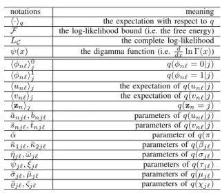
us to realize model selection, i.e., to find the optimal number of clusters. Initializing a large K cluster number, some clusters that do not have enough evidence will be pruned during the optimization process. The automatic pruning can be observed in the demo, as shown in Fig. 3.

(7)

Fig. 3. Typical run of the developed algorithm on the example data set, while the black circles represent q(μ1|k), and the red circles denote q(μ0).

The first plot shows the data set on the first two dimensions, while the last plot shows the estimation of the third and fourth dimensions.

Since the VB algorithm is proven to be monotonically increasing, it is thus able to terminate the algorithm if there is a small difference (in line 1) between consecutive iterations. In our implementation, we set =1.0−7_.

G. Interpreting the Model

Considering the time complexity of the algorithm, per iteration, computing the parameters of the posteriors of un,zn, andnareO(N d K), while for q(vn|zn), the time complexity isO(N d). Therefore, the total time complexity is ofO(N K d).

As claimed, the proposed model is supposed to deal with outliers, and to find most informative features. To detect outliers, the weighted expectation of the posteriors of un

and vn can be used as the outlier criterion. That is, if we define cn= j znj φn1j ¯ an j ¯ bn j + φn0j ¯ sn j ¯ tn j

then the smaller the value of cn with respect to yn, the higher chance that the datum is an outlier.

As stated in the model, the expectation of the feature saliency variableβj,1≤ ≤d can be applied to show the informative degree of the features for each cluster, which can be obtained as follows:

βj = κ1 j¯ ¯

κ1 j+ ¯κ2 j.

The higher theβjvalue, the more important of featurein class j .

For the overall feature saliency, we can use the following quantity to specify: ς= j πjqβj = j ˆ αj kαˆkβj

which is a weighted average over the feature saliency for each cluster. The higher theς value, the more relevant the feature.

IV. EXPERIMENTS

A. Synthetic Data

In this section, we justify the developed model and the tree-like VB algorithm using controlled experiments. Synthetic data sets are generated that are able to accommodate the data characteristics for the justification. The proposed model and the algorithm were compared with the semi-Bayesian feature selection model and algorithm, called varFnMS [34], in which a finite mixture of Gaussian is adopted and a full-factorized VB is applied.

Synthetic data are generated by first sampling a set of data points from four well-separated bivariate clusters. The centers and the variance–covariance matrices are [0 3], [1 9],

[6 4],[7 10], and an identity matrix. Eight “noisy” features [sampled from N(0,1)] are then appended to this data, resulting in a 10-D patterns. 800 data points are generated, and a set of outliers uniformly sampled from[−10 30]10 are added to the data set. Various percentages of outliers are added to the main data sets to test the performance of the algorithm on outlier detection.

The proposed algorithm was carried out for ten times with an initial cluster number K = 10. The K -means clustering algorithm is used to initialize the mean of the posterior q(μj),

(8)

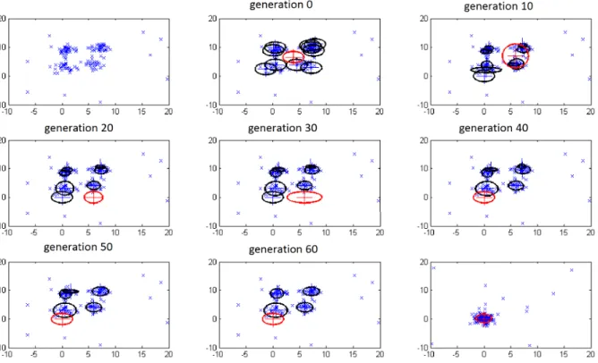
Fig. 4. Left: typical run of the semi-Bayesian feature selection algorithm, and first and second features are shown. Right: AUC values obtained by the developed algorithm and varFnMS for different percentages of outliers with standard deviations shown.

Fig. 5. Feature saliencies for the synthetic data with 5% percentage of outliers by the proposed algorithm (on the left) and the semi-Bayesian algorithm (on the right). The standard deviations of the ten runs were also shown in the plots.

and the feature saliency variable is initialized to be 0.5. The hyperparameters κ1, κ2, λ0, and α0 are set to be 10−5_{, and}

m0is set to be the mean of all data. The algorithm terminates when the difference of log-likelihood bound is less than 10−7. Fig. 3 shows a typical run of the developed algorithm, while the estimated mean and covariance of q(μ)in the first break two-dimension is shown at certain iterations. From the figure, we can see that the developed algorithm groups the data accu-rately. Moreover, it can be seen that unnecessary components are pruned automatically during the optimization process. The last plot shows the data in the third and fourth variables. The red circle demonstrates the contour of the posterior q(χ) at the third and fourth features. Fig. 4(a) shows the results obtained by varFnMS at the first and second features. From the figure, it can be seen that varFnMS is not able to eliminate the effects of the outliers, and the number of clusters has not been estimated accurately.

To test the outlier detection performance, the area under curve (AUC) values obtained through the ROC analysis can be used. The higher the AUC values, the better the perfor-mance of outlier detection. Fig. 4(b) shows the obtained AUC

values with standard deviation by the developed algorithm for different percentages of outliers in ten runs. Unfortunately, no statistics can be derived by varFnMS for the purpose of outlier detection. From the figure, it can be observed that the developed algorithm is able to pick outliers successfully. This shows that the proposed algorithm is able to simultaneously pickup outliers from the data, and discover clusters accurately. Fig. 5 shows the feature saliency retrieved by the proposed algorithm and varFnMS. From the figure, we can see that the saliency of the noisy variables (Y3−Y8) obtained by the proposed algorithm is closer to the ground truth than that of the semi-Bayesian algorithm.

B. Experiments on Real Data Sets

In this section, we used the “multiple feature database” [34], [46], which consists of features of handwritten numerals (“0”–“9”) extracted from a collection of Dutch utility maps. There are a total of 2000 images with 200 for each numerals. Numerals are represented in different feature sets. We used the same three data sets as in [34], that is, the Zernike moments (47 features), the Fourier coefficients (76 features),

(9)

TABLE III

AVERAGEDCLASSIFICATIONERROR AND THENUMBER OFCOMPONENTSOBTAINED BYvarFnMSAND THEPROPOSED ALGORITHMUSING30AND50 INITIALCOMPONENTS

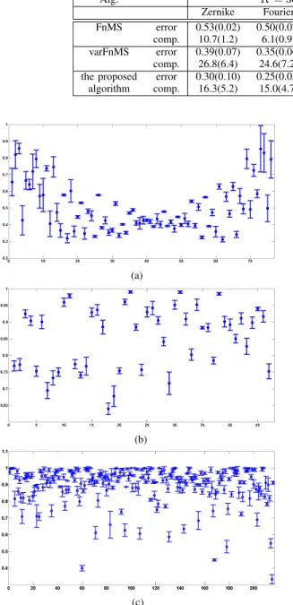
Fig. 6. Saliencies of different feature sets. (a) Fourier coefficients, (b) Zernike moments, and (c) profile correlations using the developed algorithm for models initialized with 30 components.

and profile correlations (216 features). The classification error is used to measure the performance. For each data point, it is assigned to the class with the largest responsibility. The proposed algorithm was run 20 times, where the data set is split into half to create the training and test data set. The estimated classification error and the number of components are summarized in Table III, where the components were initialized to be 30 and 50.

From Table III, we can see that our algorithm outperforms varFnMS and FnMS [46] in terms of classification error. It can be seen that the developed algorithm uses less num-ber of components than that of varFnMS, which is closer

TABLE IV

CONFUSIONMATRIXOBTAINED BY THEDEVELOPED ALGORITHM ON THELEUKEMIADATA

TABLE V

CORRELATIONBETWEEN THESTATISTICSOBTAINED IN[47]AND THE FEATURESALIENCIESWITHRESPECT TO THELEUKEMIASUBTYPES

to the true number of components. This suggests that the developed algorithm performs better in terms of recovering the true parameters. Fig. 6 shows the error bar plots of the saliencies obtained for the proposed model initialized with 30 components. As an comparison, Fig. 7 showed the salien-cies by using varFnMS with the same experimental settings as the developed algorithm. From the figure, we can see that on the Fourier coefficient data set and the profile correlation data set, the feature saliency obtained by the developed algorithm has similar trends as that of varFnMS, but of smaller variances. On the Zernike moments data set, we can see that the variances of the feature saliency revealed by the developed algorithm are much less than those obtained by varFnMS. This shows that the developed algorithm is more robust than that of varFnMS.

C. Application on High-Dimensional Gene Expression Data

In this section, we apply the developed algorithm to a large-scale gene expression data set on leukemia [47]. The data were obtained through the diagnostic of bone mar-row samples from pediatric acute leukemia (ALL) patients corresponding to six prognostically important leukemia subtypes, including 43 T-lineage ALL, 27 E2A-PBX1, 15 BCR-ABL, 79 TEL-AML1, and 20 MLL rearrangements and 64 “hyperdiploid > 50” chromosomes, and containing more than 12 600 probe sets. The resultant data set contains 248 samples, and 12 625 gene expressions. Note that in [47],

(10)

Fig. 7. Saliencies of different feature sets. (a) Fourier coefficients, (b) Zernike moments, and (c) profile correlations using varFnMS for models initialized with 30 components; reproduced from [34].

TABLE VI

EVALUATION OF THELOG-LIKELIHOODBOUND

a 2-D hierarchical clustering algorithm is first performed. The six subtypes are then recognized through the clustering results. A variety of statistical metrics (includingχ2 and t-statistics) are used to select discriminating genes for the subtypes.

We apply the developed algorithm to the data set to test if the developed algorithm is able to cluster the data accurately, and to find out the discriminating genes in the subtypes. Table IV shows the confusion matrix obtained by the devel-oped algorithm given K = 6. From Table IV, we can see that the developed algorithm agrees with the clustering results in [47] quite accurately.

On the other hand, we want to justify whether the feature saliency criterionβj,1≤≤d can be used to discriminate the genes in each class j .1 Since these values are defined to show the relevance of the features, or in the leukemia

1_{Note that in our method, we use a localized feature saliency rather than}

a global feature saliency as developed in [34] and [37]. This enables us to discriminate genes at different clusters.

clustering context, these values indicate the relevance of the genes to describe the clusters. Thus, it is expected that the feature saliency values obtained by the developed algorithm can also be used to discriminate genes for the cancer subtypes. Here, we use the correlation between the feature saliency and the statistics to evaluate the usefulness of the feature saliency values on discriminate the clusters, which will imply the performance of the developed algorithm.

To measure the correlation between the feature saliency values and the statistics, we use the Pearson correlation coefficients. Table V lists the average coefficients obtained by running the developed algorithm for ten times. From the table, we can see that the absolute values of these statistics and the feature saliency obtained by the developed algorithm for the genes have fairly strong correlation; the average of the coefficients is as high as 0.851, and no less than 0.613. This implies a coherence between the developed method and the method in [47] in terms of selecting discriminating genes.

(11)

V. CONCLUSION

In this paper, we developed a hierarchical latent variable model for feature selection and robust clustering. A full Bayesian treatment was adopted for model selection. A VB framework was used for inference. To make the inference much efficient, a tree-structured factorization of the auxiliary posteriors for the latent variables was adopted which has been shown better than the widely used full factorization approach. Quantities are proposed to detect outliers and estimate feature saliency. Controlled experiments on synthetic and real data showed that the proposed model is able to realize outlier detection and feature selection more robustly than a semi-Bayesian mixture of Gaussians model. The application of the developed algorithm to real high-dimensional data shows its applicability. In the future, unsupervised feature selection analysis on data with “big dimensionality” (i.e., the feature size is normally far beyond 10k as reviewed in [3]) is our primary research avenue. The development and the application of feature selection algorithms in broadcasting [48], cloud computing [49], image processing [50], and other areas are another avenue.

APPENDIXA

In this section, we present the derivation of the posterior distribution with respect to un,1≤n≤ N . The derivation for the other latent variables and parameters is similar.

Fq₍un|k)= log p(yn,hn)q− log q(un|zn)q.

Discarding terms that are independent of un, and using the Lagrange multiplier method, the functional to be maximized is the following: Fun|k =q(zn=k)log p(yn|un,k)p(un|k)q −q(zn=k)log q(un|k)q+λ q(un|k)dun−1 . Note here the expectation is computed with respect to the probability density functions of the parameters

Taking derivatives of Fun|k with respect to q(un|k)andλ,

q(un|k)=

exp(E(un,k)) exp1−_q₍_zλ

n=k)

(18)

then taking integral with respect to q(un|k)on both sides, we have λ=q(zn=k) 1−log ! exp(E(un,k)) " . (19) Finally, replacing (19) into (18), we obtain

q(un|k)= exp(

E(un,k))

exp(E(un,k))dun.

Note that the dimensions of the latent variable un are inde-pendent, we can then obtain

APPENDIXB

The evaluation of the free energy is presented here. Note that the main evaluation is on the computation of the expectations of the logarithms of the prior distribu-tions for the latent variables [including p(yn|un,j),p(un|j),

p(yn|vn),p(vn), p(n|β)]; the parameters [including p(β),

p(π), p(σ), p(μ), p(ξ), p(τ)]; the posteriors

[includ-ing q(un|zn),q(vn),q(zn),q(π),q(β),q(τ),q(μ),q(σ), and

q(χ)]. The evaluation of these expectations is summarized in

Table VI.

ACKNOWLEDGMENT

The authors would like to thank anonymous reviewers for their constructive and helpful comments.

REFERENCES

[1] X. Lu, Y. Wang, and Y. Yuan, “Sparse coding from a Bayesian perspective,” IEEE Trans. Neural Netw. Learn. Syst., vol. 24, no. 6, pp. 929–939, Jun. 2013.

[2] L. Shao, L. Liu, and X. Li, “Feature learning for image classification via multiobjective genetic progamming,” IEEE Trans. Neural Netw. Learn. Syst., vol. 25, no. 7, pp. 1359–1371, Jul. 2014.

[3] Y. Zhai, Y.-S. Ong, and I. Tsang, “The emerging ‘big dimensionality,”’ IEEE Comput. Intell. Mag., vol. 9, no. 3, pp. 14–26, Aug. 2014. [4] J. G. Dy and C. E. Brodley, “Feature selection for unsupervised

learning,” J. Mach. Learn. Res., vol. 5, pp. 845–889, Aug. 2004. [5] L. Laporte, R. Flamary, S. Canu, S. Déjean, and J. Mothe, “Nonconvex

regularizations for feature selection in ranking with sparse SVM,” IEEE Trans. Neural Netw. Learn. Syst., vol. 25, no. 6, pp. 1118–1130, Jun. 2014.

[6] R. Chakraborty and N. R. Pal, “Feature selection using a neural frame-work with controlled redundancy,” IEEE Trans. Neural Netw. Learn. Syst., vol. 26, no. 1, pp. 35–49, Jan. 2015.

[7] Y. Li, J. Si, G. Zhou, S. Huang, and S. Chen, “FREL: A stable feature selection algorithm,” IEEE Trans. Neural Netw. Learn. Syst., vol. 26, no. 7, pp. 1388–1402, Jul. 2015.

[8] T. Naghibi, S. Hoffmann, and B. Pfister, “A semidefinite programming based search strategy for feature selection with mutual information measure,” IEEE Trans. Pattern Anal. Mach. Intell., vol. 37, no. 8, pp. 1529–1541, Aug. 2016.

[9] H. Tao, C. Hou, F. Nie, Y. Jiao, and D. Yi, “Effective discriminative feature selection with nontrivial solution,” IEEE Trans. Neural Netw. Learn. Syst., vol. 27, no. 4, pp. 796–808, Apr. 2016.

[10] P. Padungweang, C. Lursinsap, and K. Sunat, “A discrimination analy-sis for unsupervised feature selection via optic diffraction principle,” IEEE Trans. Neural Netw. Learn. Syst., vol. 23, no. 10, pp. 1587–1600, Oct. 2012.

[11] Z. Zhao, L. Wang, H. Liu, and J. Ye, “On similarity preserving feature selection,” IEEE Trans. Knowl. Data Eng., vol. 25, no. 3, pp. 619–632, Mar. 2013.

(12)

[12] S. Wang, W. Pedrycz, Q. Zhu, and W. Zhu, “Unsupervised fea-ture selection via maximum projection and minimum redundancy,” Knowl.-Based Syst., vol. 75, pp. 19–29, Feb. 2015.

[13] J. Yao, Q. Mao, S. Goodison, V. Mai, and Y. Sun, “Feature selection for unsupervised learning through local learning,” Pattern Recognit. Lett., vol. 53, pp. 100–107, Feb. 2015.

[14] Z. Zhao, X. He, D. Cai, L. Zhang, W. Ng, and Y. Zhuang, “Graph regularized feature selection with data reconstruction,” IEEE Trans. Knowl. Data Eng., vol. 28, no. 3, pp. 689–700, Mar. 2016.

[15] X. Zhu, X. Li, S. Zhang, C. Ju, and X. Wu, “Robust joint graph sparse coding for unsupervised spectral feature selection,” IEEE Trans. Neural Netw. Learn. Syst., to be published, doi: 10.1109/TNNLS.2016.2521602. [16] Z. Xu, I. King, M. R.-T. Lyu, and R. Jin, “Discriminative semi-supervised feature selection via manifold regularization,” IEEE Trans. Neural Netw., vol. 21, no. 7, pp. 1033–1047, Jul. 2010.

[17] X. Liu, L. Wang, J. Zhang, J. Yin, and H. Liu, “Global and local structure preservation for feature selection,” IEEE Trans. Neural Netw. Learn. Syst., vol. 25, no. 6, pp. 1083–1095, Jun. 2014.

[18] X. He, D. Cai, and P. Niyogi, “Laplacian score for feature selection,” in Proc. NIPS, 2005, pp. 80–87.

[19] Y. Jiang and J. Ren, “Eigenvalue sensitive feature selection,” in Proc. 28th ICML, 2011, pp. 89–96.

[20] M. Sebban and R. Nock, “A hybrid filter/wrapper approach of feature selection using information theory,” Pattern Recognit., vol. 35, no. 4, pp. 835–846, 2002.

[21] L. Yu and H. Liu, “Feature selection for high-dimensional data: A fast correlation-based filter solution,” in Proc. 20th Int. Conf. Mach. Learn., 2003, pp. 856–863.

[22] A. Arauzo-Azofra, J. M. Benitez, and J. L. Castro, “Consistency measures for feature selection,” J. Intell. Inf. Syst., vol. 30, no. 3, pp. 273–292, 2007.

[23] Q. Gu and J. Zhou, “Local learning regularized nonnegative matrix factorization,” in Proc. 21st Int. Joint Conf. Artif. Intell., 2009, pp. 1–6. [24] H. Zeng and Y.-M. Cheung, “Feature selection and kernel learning for local learning-based clustering,” IEEE Trans. Pattern Anal. Mach. Intell., vol. 33, no. 8, pp. 1532–1547, Aug. 2011.

[25] A. Ng, “Feature selection, L1 vs. L2 regularization, and rotational

invariance,” in Proc. 21st Int. Conf. Mach. Learn., 2004, p. 78. [26] Y. Yang, H. Shen, Z. Ma, and Z. Huang, “2,1-norm regularized

discriminative feature selection for unsupervised learning,” in Proc. 22nd Int. Joint Conf. Artif. Intell., 2011, pp. 1–6.

[27] F. Nie, H. Huang, X. Cai, and C. Ding, “Efficient and robust feature selection via joint2,1-norms minimization,” in Proc. Adv. Neural Inf.

Process. Syst., vol. 23. 2010, pp. 1813–1821.

[28] Z. Li, Y. Yang, J. Liu, X. Zhou, and H. Lu, “Unsupervised feature selection using nonnegative spectral analysis,” in Proc. 26th AAAI Conf. Artif. Intell., 2012, pp. 1–7.

[29] Z. Zhao and H. Liu, “Semi-supervised feature selection via spectral analysis,” in Proc. 7th SIAM Int. Conf. Data Mining, 2007.

[30] Z. Zhao and H. Liu, “Spectral feature selection for supervised and unsupervised learning,” in Proc. 24th ICML, 2007, pp. 1151–1157. [31] Z. Li, J. Liu, Y. Yang, X. Zhou, and H. Lu, “Clustering-guided sparse

structural learning for unsupervised feature selection,” IEEE Trans. Knowl. Data Eng., vol. 26, no. 9, pp. 2138–2150, Sep. 2014. [32] C. Hou, F. Nie, X. Li, D. Yi, and Y. Wu, “Joint embedding learning

and sparse regression: A framework for unsupervised feature selection,” IEEE Trans. Cybern., vol. 44, no. 6, pp. 793–804, Jun. 2014. [33] S. H. Yang and B. G. Hu, “Discriminative feature selection by

non-parametric Bayes error minimization,” IEEE Trans. Knowl. Data Eng., vol. 24, no. 8, pp. 1422–1434, Aug. 2012.

[34] C. Constantinopoulos, M. K. Titsia, and A. Likas, “Bayesian feature and model selection for Gaussian mixture models,” IEEE Trans. Pattern Anal. Mach. Intell., vol. 28, no. 6, pp. 1013–1018, Jun. 2006. [35] P. Carbonetto, N. de Freitas, P. Gustafson, and N. Thompson, “Bayesian

feature weighting for unsupervised learning, with application to object recognition,” in Proc. 9th Int. Conf. Artif. Intell. Statist., 2003. [36] W. Pan and X. Shen, “Penalized model-based clustering with application

to variable selection,” J. Mach. Learn. Res., vol. 8, pp. 1145–1164, May 2007.

[37] M. H. C. Law, M. A. T. Figueiredo, and A. K. Jain, “Simulta-neous feature selection and clustering using mixture models,” IEEE Trans. Pattern Anal. Mach. Intell., vol. 26, no. 9, pp. 1154–1166, Sep. 2004.

[38] Y. Li, M. Dong, and J. Hua, “Simultaneous localized feature selec-tion and model detecselec-tion of Gaussian mixtures,” IEEE Trans. Pattern Recognit. Mach. Intell., vol. 31, no. 5, pp. 953–960, May 2009.

[39] J. Sun, A. Kabán, and S. Raychaudhury, “Robust mixtures in the presence of measurement errors,” in Proc. 24th Int. Conf. Mach. Learn., Corvallis, OR, USA, 2007, pp. 847–854.

[40] J. Sun, A. Kaban, and J. Garibaldi, “Robust mixture modeling using the Pearson type VII distribution,” Pattern Recognit. Lett., vol. 31, no. 16, pp. 2447–2454, 2010.

[41] G. McLachlan and D. Peel, Finite Mixture Models. Hoboken, NJ, USA: Wiley, 2000.

[42] C. Bishop, Pattern Recognition and Machine Learning. Springer, 2006. [43] D. Blei and M. I. Jordan, “Variational inference for Dirichlet process mixtures,” Int. Soc. Bayesian Anal., Durham, USA, vol. 1, no. 1, pp. 121–144, 2006.

[44] J. Sun and A. Kaban, “A fast algorithm for robust mixtures in the presence of measurement errors,” IEEE Trans. Neural Netw., vol. 21, no. 8, pp. 1206–1220, Aug. 2010.

[45] J. Sun, J. Garibaldi, and K. Kenobi, “Robust Bayesian clustering for datasets with repeated measures,” IEEE/ACM Trans. Comput. Biol. Bioinformatics, vol. 9, no. 5, pp. 1504–1514, Sep. 2012.

[46] A. Jain, R. P. W. Duin, and J. Mao, “Statistical pattern recognition: A review,” IEEE Trans. Pattern Anal. Mach. Learn., vol. 22, no. 1, pp. 4–38, Jan. 2000.

[47] E.-J. Yeoh et al., “Classification, subtype discovery, and prediction of outcome in pediatric acute lymphoblastic leukemia by gene expression profiling,” Cancer Cell, vol. 1, no. 2, pp. 133–143, 2002.

[48] Z. Pan, J. Lei, Y. Zhang, X. Sun, and S. Kwong, “Fast motion estimation based on content property for low-complexity h.265/hevc encoder,” IEEE Trans. Broadcast., vol. 62, no. 3, pp. 675–684, Sep. 2016. [49] Z. Fu, X. Sun, Q. Liu, L. Zhou, and J. Shu, “Achieving efficient cloud

search services: Multi-keyword ranked search over encrypted cloud data supporting parallel computing,” IEICE Trans. Commun., vol. E98-B, no. 1, pp. 190–200, 2015.

[50] Y. Zheng, J. Byeungwoo, D. Xu, Q. M. J. Wu, and H. Zhang, “Image segmentation by generalized hierarchical fuzzy C-means algorithm,” J. Intell. Fuzzy Syst., vol. 28, no. 2, pp. 961–973, 2015.

Jianyong Sun received the B.Sc. degree in

computa-tional mathematics from Xi’an Jiaotong University, Xi’an, China, in 1997, and the Ph.D. degree in computer science from the University of Essex, Colchester, U.K., in 2005.

He was a Lecturer with the University of Essex and a Senior Lecturer with the University of Greenwich, London, U.K. He is currently a Professor with Xi’an Jiaotong University. He has authored over 40 peer-reviewed research papers. His current research interests include theoretical and practi-cal aspects of artificial intelligence, mainly on evolutionary computation, statistical machine learning and their applications in bioinformatics, and astro-informatics.

Aimin Zhou (S’08–M’10) received the B.Sc. and

M.Sc. degrees from Wuhan University, Wuhan, China, in 2001 and 2003, respectively, and the Ph.D. degree from the University of Essex, Colchester, U.K., in 2009, all in computer science.

He is currently an Associate Professor with the Shanghai Key Laboratory of Multidimensional Information Processing, Department of Computer Science and Technology, East China Normal Uni-versity, Shanghai, China. He has authored over 40 peer-reviewed papers. His current research inter-ests include evolutionary computation and optimisation, machine learning, image processing, and their applications.

Dr. Zhou is an Associate Editor of Swarm and Evolutionary Computation and an Editorial Board Member of Complex and Intelligent Systems.

(13)

Simeon Keates received the M.A. and Ph.D. degrees

in engineering from the Department of Engineering, University of Cambridge, Cambridge, U.K.

He was the Head of the School of Engineer-ing, Computing and Applied Mathematics, Univer-sity of Abertay Dundee, Dundee, Scotland, and an Associate Professor with the IT University of Copenhagen, Copenhagen, Denmark, where he lec-tured in the Design and Digital Communication study line. He was an Industrial Research Fellow with the Engineering Design Centre, University of Cambridge, supported by Royal Mail. He joined the Accessibility Research Group, IBM TJ Watson Research Center. He was with ITA Software as a Usability Lead designing interfaces for Air Canada. He is currently the Deputy Pro Vice Chancellor with the Faculty of Engineering and Science, University of Greenwich, London, U.K., where he is responsible for strategic management of Engineering and also for industrial engagement. He also has an extensive history of consultancy, with clients including Royal Mail, the US Social Security Administration, the U.K. Department of Trade and Industry, Danish Broadcasting Corporation (Danske Radio) and Lockheed Martin.

Dr. Keates was the Chair of HCI.

Shengbin Liao received the Ph.D. degree from the

Department of Electronics and Information Engi-neering, Huazhong University of Science and Tech-nology, Wuhan, China, in 2008.

He is currently an Associate Professor with the National Engineering Research Center for E-Learning, Huazhong Normal University, Wuhan. His current research interests include machine learn-ing and big data, distributed optimization and con-trol, and automated problem solving based on deep learning.