Pooling versus model selection for
nowcasting with many predictors:
an application to German GDP
Vladimir Kuzin
(DIW)
Massimiliano Marcellino
(EUI, Università Bocconi and CEPR)
Christian Schumacher
(Deutsche Bundesbank)
Discussion Paper
Series 1: Economic Studies
No 03/2009
Editorial Board: Heinz Herrmann
Thilo Liebig
Karl-Heinz Tödter
Deutsche Bundesbank, Wilhelm-Epstein-Strasse 14, 60431 Frankfurt am Main, Postfach 10 06 02, 60006 Frankfurt am Main
Tel +49 69 9566-0
Telex within Germany 41227, telex from abroad 414431 Please address all orders in writing to: Deutsche Bundesbank,
Press and Public Relations Division, at the above address or via fax +49 69 9566-3077
Internet http://www.bundesbank.de
Reproduction permitted only if source is stated. ISBN 978-3–86558–487–8 (Printversion) ISBN 978-3–86558–488–5 (Internetversion)
Abstract
This paper discusses pooling versus model selection for now- and forecasting in the pres-ence of model uncertainty with large, unbalanced datasets. Empirically, unbalanced data is pervasive in economics and typically due to di¤erent sampling frequencies and publication delays. Two model classes suited in this context are factor models based on large datasets and mixed-data sampling (MIDAS) regressions with few predictors. The speci…cation of these models requires several choices related to, amongst others, the factor estimation method and the number of factors, lag length and indicator selection. Thus, there are many sources of mis-speci…cation when selecting a particular model, and an alternative could be pooling over a large set of models with di¤erent speci…ca-tions. We evaluate the relative performance of pooling and model selection for now-and forecasting quarterly German GDP, a key macroeconomic indicator for the largest country in the euro area, with a large set of about one hundred monthly indicators. Our empirical …ndings provide strong support for pooling over many speci…cations rather than selecting a speci…c model.
Keywords: nowcasting, forecast combination, forecast pooling, model selection, mixed-frequency data, factor models, MIDAS
Non-technical summary
In this paper, we evaluate the empirical performance of new short-term forecasting methods with respect to now- and forecasting of German GDP. In general, forecasting in real-time is subject to considerable uncertainty, and in our forecast exercise, we particularly account for two types of uncertainty: the uncertainty regarding the choice of the appropriate forecasting model and the uncertainty about the relevant business cycle indicators to be included in the model. In our paper, we consider forecast pooling methods to tackle both sources of forecast uncertainty. In the empirical literature, forecast combinations are considered as useful forecast tools, as they can insure against choosing an inappropriate single model by sharing the risk of model mis-speci…cation between many models. In an empirical forecast comparison, we compare pooling to alternative methods of model selection for forecasting. We employ two alternative classes of econometric models to compute now- and forecasts: factor models based on large datasets and mixed-data sampling (MIDAS) regressions based on a few predictors. To evaluate the impact of mis-speci…cation on the forecast accuracy, we compare ex-post and ex-ante forecasts. Ex-ex-post forecasts are based on …xed model speci…cations that have been selected after inspecting their performance in a recursive comparison. Ex-ante forecasts, however, are based on models that have been speci…ed without referring to forecast errors that are only known ex post. Thus, the ex-ante forecasts are better suited for a more realistic assessment of the model’s performance. The ex-post forecasts provide stylised results based on optimised model structures that are not subject to model uncertainty. Thus, a comparison between ex-post and ex-ante forecasts isolate the e¤ect of mis-speci…cation on the forecast performance.
An novel aspect of the current paper compared to the existing literature on forecast pooling is the explicit and model-consistent consideration of unbalanced datasets. In short-term forecasting exercises, there are often two relevant phenomena that lead to unbalanced datasets: …rst, the di¤erent sampling frequencies of the data, and, second, the missing observations at the end of the sample due to di¤erent publication lags, the so-called ‘ragged edge’in multivariate data. For example, interest rates are typically observed at higher frequency and much more timely than variables like GDP or other national accounts data.
Short-term forecasts often refer to current-quarter forecasts and forecasts one-quarter ahead. In spite of these relatively short forecast horizons, the forecasts are subject to considerable uncertainty. One important reason for this is that the informa-tion content of forecasts from a particular model is often not constant over time due to structural instabilities, which is a common …nding from the literature. Hence, it can be the case, that a model performs well in a particular evaluation period, but performs worse in another evaluation period after a structural break has occurred. One way to tackle this problem is by means of forecast pooling, which implies constructing a
com-bined forecast from the output of a set of di¤erent forecasting models. An alternative to pooling is model selection based on statistical information criteria.
The empirical …ndings for German GDP show the existence of many particular models and leading indicators that perform very well on an ex post basis. However, this holds only if the optimal model structure and relevant leading indicator is known, that is the framework of ex-post forecasts. In the case of ex-ante forecasts, without knowledge regarding the optimal model structure, the forecasting performance deteri-orates dramatically when model selection based on information criteria is employed. On the contrary, forecast pooling performs well overall. Although some of the indi-vidual best-performing models do better than the combinations, the majority of single models is generally outperformed. Furthermore, the forecasting power of single leading indicators and models turned out to change over time, whereas forecast combinations were stable overall. These results suggest that forecast pooling is a reliable and robust tool for short-term forecasting of macroeconomic activity.
Nicht-technische Zusammenfassung
Im vorliegenden Beitrag wird untersucht, wie gut neuere Kurzfristprognoseverfahren die Entwicklung des deutschen Bruttoinlandsprodukts (BIP) vorhersagen können. Dabei wird berücksichtigt, dass Unsicherheit sowohl bezüglich der Auswahl der Form des geeigneten Prognosemodells besteht, als auch hinsichtlich der Auswahl der zu berück-sichtigenden makroökonomischen Variablen, welche Informationen über die künftige Wirtschaftsentwicklung liefern sollen. Um diese Unsicherheiten bei der Prognoseer-stellung zu berücksichtigen, werden in diesem Beitrag alternative Verfahren der Prog-nosekombination (forecast pooling) angewendet. Kombinationen von Prognosen streuen das Risiko von Fehlspezi…kationen einzelner Modelle und haben sich in der Literatur als vielversprechende Prognoseinstrumente etabliert. In einem empirischen Progno-severgleich werden die Prognosekombinationen mit den Vorhersagen einzelner Modelle verglichen, wobei die Auswahl des geeigneten Modells als auch der relevanten Predik-toren mit unterschiedlichen Ansätzen erfolgt. Für die vorliegende Analyse werden zwei alternative Klassen ökonometrischer Modelle aus der jüngeren Literatur herangezogen: große Faktormodelle mit großen Datensätzen und Modelle auf Basis des sog. MIDAS-Regressionsansatzes mit wenigen Prediktoren. Um den Ein‡uss von Fehlspezi…katio-nen auf das Prognoseergebnis bei diesen Modellklassen zu evaluieren, vergleicht das Papier die Ergebnisse auf der Basis von ex-post und ex-ante Prognosen. Ex-post Prog-nosen basieren auf …xen Modellspezi…kationen, die nach Durchführung eines rekursiven Prognosevergleichs anhand ihrer dort erreichten Prognoseleistung ausgewählt wurden. Ex-ante Prognosen basieren hingegen auf Modellen, welche ohne Rückgri¤ auf lediglich ex post bekannte Prognoseergebnisse spezi…ziert werden und daher für eine realistis-che Beurteilung unter Modellunsirealistis-cherheit angemessener sind. Die ex-post Prognosen zeigen idealisierte Ergebnisse auf Basis einer optimierten Modellstruktur ohne Model-lunsicherheit bei Kenntnis der Prognosefehler, so dass ein Vergleich zwischen ex-post und ex-ante Prognosen den Ein‡uss von Fehlspezi…kationen aufzeigt.
Im Vergleich zu anderen Arbeiten auf dem Gebiet der Prognosekombination berück-sichtigt die vorliegende Arbeit explizit und modellkonsistent, dass bei der Prognose Daten üblicherweise "unbalanciert" zur Verfügung stehen: Insbesondere weisen die verwendeten Daten unterschiedliche Frequenzen auf und sind am aktuellen Rand we-gen Publikationsverzögerunwe-gen nur unvollständig verfügbar (ragged-edge Problematik). Beispielsweise sind Zinssätze oder andere Finanzmarktdaten mit höherer Frequenz und wesentlich früher verfügbar als die viele Daten der volkswirtschaftlichen Gesamtrech-nung. So ist das BIP nur als Quartalsangabe und mit erheblicher Zeitverzögerung verfügbar.
Die Kurzfristprognosen beziehen sich auf das laufende oder das folgende Quartal. Trotz dieses kurzen Prognosezeitraums sind sie meist mit erheblichen Unsicherheiten verbunden. In Prognosevergleichen tritt nämlich aufgrund von strukturellen
Instabil-itäten oftmals der Fall ein, dass ein Vorhersagemodell keine beständig gute Prognose-leistung erbringt, also in einer bestimmten Prognoseperiode relativ gut im Vergleich zu anderen Modellen abschneidet und infolge von Strukturbrüchen relativ schlecht in anderen Perioden. Durch die Kombination unterschiedlicher Prognosemodelle versucht man dieses Problem zu mindern. Alternativ können statistische Informationskriterien verwendet werden um einzelne Prognosemodelle auszuwählen.
In der empirischen Anwendung für das deutsche BIP zeigt sich, dass durchaus eine Vielzahl von Einzelmodellen und Frühindikatoren mit beachtlicher Prognosegüte gefunden werden können. Dies gilt jedoch nur bei Kenntnis der optimalen Modell-struktur und der relevanten Konjunkturindikatoren als Prediktoren, d.h., bei ex-post Prognosen. Bei ex-ante Prognosen, also wenn die optimale Struktur des Prognosemod-ells nicht bekannt ist und beispielsweise mit Informationskriterien bestimmt werden muss, nimmt die Prognosegüte der Einzelmodelle aber dramatisch ab. Dagegen liefern die Prognosekombinationen gute Ergebnisse unter ex-ante Bedingungen. Zwar können die kombinierten Prognosen die besten ex-post ausgewählten Einzelmodelle in der Regel nicht übertre¤en, jedoch liegen ihre Prognosefehler deutlich unter der großen Mehrzahl der meisten Einzelmodelle. Ferner zeigt sich, dass die Prognosegüte einzelner Konjunk-turindikatoren im Zeitablauf schwankt, während die Kombinationen stabile Ergebnisse aufweisen. Diese Ergebnisse legen den Schluss nahe, dass kombinierte Prognosen als nützlich für Kurzfristprognosen anzusehen sind.
Contents
1 Introduction 1
2 Nowcasting quarterly GDP with ragged-edge data: MIDAS, factor
models, and pooling 4
2.1 The MIDAS approach as a now- and forecasting tool . . . 4
2.2 The MIDAS predictors . . . 7
2.2.1 MIDAS forecasting with a single indicator . . . 7
2.2.2 MIDAS forecasting with factors . . . 7
2.3 Nowcast pooling over many speci…cations of models . . . 10
3 Design of the nowcast and forecast comparison exercise 12 3.1 Data and replication of the ragged edge . . . 12
3.2 Nowcast and forecast design . . . 13
3.3 Speci…cation of MIDAS and factor models . . . 14
4 Now- and forecasts from single models 15 4.1 Fixed speci…cations . . . 16
4.2 Information-criteria model selection and speci…cation based on past per-formance . . . 18
5 Nowcast pooling 19 6 Robustness of the results 22 6.1 Subsample analysis . . . 22
6.2 Double-indicator MIDAS . . . 23
6.3 BIC speci…cation of Factor-MIDAS . . . 24
7 Conclusions 24 A Monthly dataset 29 A.1 Prices . . . 30
A.2 Labour market . . . 30
A.3 Interest rates, stock market indices . . . 31
A.4 Manufacturing turnover, production and received orders . . . 31
A.5 Construction . . . 32
A.6 Surveys . . . 33
A.7 Miscellaneous indicators . . . 33
B The two-step factor estimator by Forni et al. (2005) 34
Pooling versus model selection for nowcasting with many
predictors: An application to German GDP
y1
Introduction
Forecast models that can take into account unbalanced datasets have received sub-stantial attention in the recent literature. In real time, the unbalancedness of datasets arises due to the di¤erent sampling frequencies and di¤erent publication delays of busi-ness cycle indicators. For example, Gross Domestic Product (GDP), a key indicator of macroeconomic activity, is typically published at quarterly frequency and has a consid-erable publication lag. As policy makers regularly request information on the current state of the economy in terms of GDP, there is a need to provide estimates of current GDP in order to support policy decisions. Following the discussion in Giannone et al. (2008), we call the necessary projection of current GDP the ‘nowcast’ in this paper. In the same way, other business cycle indicators, that might serve as predictors for GDP, are released in an asynchronous way and exhibit complicated patterns of missing values at the end of the sample, which leads to the so-called ‘ragged-edge’problem of multivariate data in econometrics, see Wallis (1986). Another di¢ culty arises, because GDP is released on a quarterly basis, whereas many important predictors are sampled at monthly or higher frequencies. Therefore, now- and forecast models should be able to account for mixed-frequency and ragged-edge data.
In the recent forecast literature, two alternative modeling approaches that can take into account these data irregularities have been discussed: mixed-data sampling (MI-DAS) regressions with a few indicators and large factor models. In the MIDAS ap-proach, as introduced by Ghysels and Valkanov (2006) and Ghysels, Sinko and Valka-nov (2007), a low-frequency variable is regressed on higher frequency variables using skip-sampling and restricted lag polynomials. Clements and Galvão (2008, 2009) in-troduced the MIDAS approach to macroeconomics, and presented empirical results for US quarterly GDP predicted by monthly indicators. Due to the skip-sampling
yThis paper represents the authors’personal opinions and does not necessarily re‡ect the views of
the Deutsche Bundesbank. We are grateful to seminar and workshop participants at the Bundesbank, DIW Berlin, University of Basle, and the University of Frankfurt for helpful comments. Helpful comments were also provided by Heinz Herrmann, Sylvia Kaufmann, and Karl-Heinz Tödter. The codes for this paper were written in Matlab. Some functions were taken from the Econometrics Toolbox written by James P. LeSage fromwww.spatial-econometrics.com. Other codes were kindly provided by Mario Forni fromwww.economia.unimore.it/forni_mario/matlab.htm, Arthur Sinko fromwww.unc.edu/~sinko/midas.zip, and Gerhard Rünstler.
and direct projection, MIDAS can tackle mixed-frequency data as well as di¤erences in data availability at the end of the sample. Whereas MIDAS is mainly a forecast tool based on a few selected indicators, the usefulness of factor models based on large datasets as forecast devices has been widely discussed in the recent literature, see the seminal papers by Stock and Watson (2002) and Forni et al. (2005). If ragged-edge and mixed-frequency data is present, factor estimation methods that take into proper account these data irregularities are required. Two prominent methods from the recent literature are: the two-step estimator in a state-space framework by Doz et al. (2006) and Giannone et al. (2008), which can account for statistical publication lags in the in-dicator dataset by using the Kalman smoother; and the dynamic principal components estimator by Altissimo et al. (2006), which can also handle ragged edge datasets, and thereby extends the dynamic estimator by Forni et al. (2005) based on balanced data. Within the MIDAS and factor model classes, the practitioner has to make a set of auxiliary decisions when applying them for forecasting. For example, proper indicator selection is crucial for MIDAS regressions. However, in a related framework with single-frequency data, Banerjee and Marcellino (2006) for the US and Banerjee et al. (2005) for the Euro area have found that selecting variables in real time can be much more di¢ cult than what suggested by ex-post evaluations. The factor forecast framework is also not immune to mis-speci…cation issues, e.g., there is an ongoing discussion regarding the appropriate factor estimation method, see Boivin and Ng (2005), Stock and Watson (2006), D’Agostino and Giannone (2006), and Schumacher (2007). And proper handling of dynamics is a problem for both approaches, even more than usual due to the mixed sampling frequencies of the indicators. Therefore, it is very likely that even a careful selection process can result in a mis-speci…ed model.
In the present paper, we propose nowcast pooling as a simple way of dealing with this substantial model uncertainty, exacerbated by the use of large unbalanced datasets. From a theoretical point of view, it is di¢ cult to rank model speci…cation and pooling in …nite and irregular samples. In addition, their relative performance will depend on the assumptions on the data generating process. Therefore, we prefer to take an empirical approach. In particular, we evaluate the nowcast performance of pooling and single models for quarterly German GDP, a key variable for the largest country in the euro area. Speci…cally, …rst we investigate the performance of a large number of MIDAS and factor models with di¤erent speci…cations, that are held …xed in the recursive evaluation exercise. In other words, on an ex-post basis, we search for the best speci…cations. Second, in order to allow for data-driven speci…cation, we consider real-time model selection based either on information criteria or on the past forecast performance of the individual models, following the discussion in Inoue and Kilian (2006). Finally, we discuss to what extent alternative pooling schemes can circumvent potential mis-speci…cation of single models. We consider averaging with equal weights,
the median as well as performance-based weights over full set of models. As the sample under consideration is relatively small, and simple forecast combinations have turned out to provide robust results in the literature, we do not account for more sophisticated pooling methods, see e.g. Clark and McCracken (2008).
It is well known that pooling of forecasts provides a robust tool in the presence of mis-speci…cation and parameter instability, see for example Timmermann (2005) and Clements and Hendry (2004) for theoretical results, and Clark and McCracken (2008), Assenmacher-Wesche and Pesaran (2008) and Garratt et al. (2009) for recent empirical applications. However, these papers do not take into account the data unbalancedness, which is pervasive in economics due to publication delays of statistical data and dif-ferent sampling frequencies. Instead, we focus on pooling MIDAS and factor models as econometric speci…cations that take into explicit account the data unbalancedness. Hence, our …rst original contribution to the literature is to assess pooling in a more realistic context and for models potentially more useful for empirical analysis.
Our second original contribution is to compare MIDAS regressions based on few selected indicators with factor models based on large datasets, thus relating the MIDAS literature from Clements and Galvão (2008, 2009) to the factor nowcast literature from Giannone et al. (2008), Altissimo et al. (2006) and Marcellino and Schumacher (2008).1
Our main results can be summarised as follows. First, searching in the set of all pos-sible models on an ex-post basis, it is pospos-sible to …nd MIDAS and factor speci…cations that outperform a simple benchmark, and MIDAS models with a few indicators tend to outperform factor models in this ex-post evaluation. Since the search described above is based on full sample results, it might be subject to the data-mining critique. Second, when selecting the forecasting models in real time based either on information criteria or on their past performance, it is much more di¢ cult to beat the benchmark, with the exception of factor model selection based on past forecasting performance. Third, pooling the whole set of MIDAS and factor now- and forecasts clearly outperforms single models selected according to information-criteria or based on their past perfor-mance. In comparison with the best …xed speci…cations selected on an ex-post basis, pooling is better than 93-100% of all the single indicator forecasts, and of 86-100% of all the factor forecasts, depending on the horizon. Furthermore, in real time, pooling of factor models seems to outperform pooling of MIDAS models with few indicators.
In summary, the main …nding of our paper is that there is considerable uncer-tainty with respect to the appropriate speci…cation of the compilcated econometric tools needed to handle large and unbalanced datasets of macroeconomic variables. In this context, pooling of many speci…cations within and across the MIDAS and factor
1Barhoumi et al. (2008) also consider forecasting with ragged-edge data, but do not consider
MIDAS approaches and speci…cation uncertainty as in the present paper, in particular, with respect to speci…cation uncertainty of factor models.
model classes is overall superior to selecting a single model.
The paper proceeds as follows. Section 2 provides an overview of the individual MIDAS regressions and factor models employed here, as well as the combination meth-ods. Section 3 describes the design of the forecast comparison exercise. Section 4 presents and compares the empirical results for …xed, information criteria and past performance based speci…cations. Section 5, discusses pooling over the whole set of MIDAS and Factor-MIDAS speci…cations. Section 6 conducts a variety of robustness analyses. Section 7 summarizes and concludes.
2
Nowcasting quarterly GDP with ragged-edge data:
MIDAS, factor models, and pooling
To forecast quarterly GDP using monthly indicators, we mainly rely on the mixed-data sampling (MIDAS) approach as proposed by Ghysels and Valkanov (2006), Ghysels et al. (2007), and Clements and Galvão (2008, 2009). MIDAS is a single-equation ap-proach that allows a low-frequency variable like GDP to be explained by high-frequency regressors. In our application, we will consider di¤erent types of regressors: either a small number of business cycle indicators, following the work by Clements and Galvão (2008, 2009), or factors estimated from a large set of indicators, following Marcellino and Schumacher (2008). For both types of regressors, the MIDAS regression approach serves as a way to compute the projections. Below, in subsection 2.1, we …rst introduce the MIDAS regression, then discuss the choice of monthly predictors in subsection 2.2, in particular the di¤erent factor estimation approaches that can be applied to large sets of indicators. When discussing the alternative approaches, we will also address the di¤erent speci…cations that are necessary when applying the models in real time. Finally, the alternative pooling methods are described in subsection 2.3.
2.1
The MIDAS approach as a now- and forecasting tool
In our application, the predictand is quarterly GDP growth, which is denoted as ytq wheretq is the quarterly time indextq = 1;2;3; : : : ; Tqy withTqy as the …nal quarter for
which GDP is available. GDP growth can also be expressed at the monthly frequency by setting ytm =ytq8tm = 3tq with tm as the monthly time index. Thus, GDP ytm is observed only at months tm = 3;6;9; : : : ; Tmy with Tmy = 3Tqy. The aim is to forecast
GDP hq quarters ahead, or hm = 3hq months ahead, yielding a value foryTmy+hm. Nowcasting means that in a particular calender month, we do not observe GDP for the current quarter. It can even be the case that GDP is only available with a delay of two periods. In April, for example, German GDP is only available for the fourth quarter of the previous year, and a nowcast for second quarter GDP requires hq = 2.
Thus, if a decision maker requests an estimate of current quarter GDP, the forecast horizon has to be set su¢ ciently large in order to provide the appropriate …gures. For further discussion on nowcasting, see Giannone et al. (2008).
To now- and forecast quarterly GDP growth, we can make use of a stationary monthly predictor ztm. For simplicity, we assume that there is only one predictor, and generalise this case later on to more than one indicators or factors. The time index tm
denotes a monthly period, and observations ofztm are available fortm = 1;2;3; : : : ; T
z m,
whereTz
m is the …nal month for which an observation is available. Usually, Tmz is larger
than Ty
m = 3Tqy, as monthly observations for many relevant macroeconomic indicators,
in particular …nancial or survey data, are earlier available than GDP observations. The forecast for GDP is denoted asyTy
m+hmjTmz, as we condition the forecast on information available in month Tz
m, which also includes GDP observations up to Tqy in addition
to the indicator observations up to Tz
m with Tmz Tmy = 3Tqy. Thus, the indicator is
available wzy =Tmz Tmy months ahead of GDP.
Basic MIDAS The forecast model for forecast horizon hq quarters with hq =hm=3
is
ytq+hq =ytm+hm = 0+ 1b(Lm; )z
(3)
tm+wzy +"tm+hm; (1) where wzy =Tmz Tmy and the polynomial b(Lm; )is the exponential Almon lag
b(Lm; ) = K X k=0 c(k; )Lkm; c(k; ) = exp( 1k+ 2k 2) K P k=0 exp( 1k+ 2k2) ; (2)
with the monthly lag operatorLm de…ned asLmztm =ztm 1. In the MIDAS approach, quarterly GDPytq+hq is directly related to the indicatorz
(3)
tm+j and its lags, where z
(3)
tm is a skip-sampled version of the monthly ztm. The superscript three indicates that every third observation starting from the tm-th one is included in the regressor z
(3)
tm, thusz(3)tm =ztm8tm =: : : ; T
z
m 6; Tmz 3; Tmz. Lags of the monthly factors are treated
accordingly, e.g. thek-th lagzt(3)
m k =ztm k8tm =: : : ; T
z
m k 6; Tmz k 3; Tmz k. In
the regression, the variable wzy denotes the number of monthly periods, the monthly
indicator is earlier available than GDP. Thus, we take into account that a monthly indicator is typically available within the quarter for which no GDP …gure is available, see Clements and Galvão (2008, 2009).
For given =f 1; 2g, the exponential lag function b(Lm; ) provides a
parsimo-nious way to consider monthly lags of the factors as we can allow for large K to approximate the impulse response function of GDP from the factors. The longer the lead-lag relationship in the data is, the less MIDAS su¤ers from sampling uncertainty compared with the estimation of unrestricted lags, where the number of coe¢ cients increases with the lag length.
The MIDAS model can be estimated using nonlinear least squares (NLS) in a re-gression of ytm onto z
(3)
tm+wzy hm and lags, yielding coe¢ cients b1, b2, b0 and b1. The forecast is given by
yTy
m+hmjTmz = b0+b1b(Lm;b)zTmz: (3) According to this forecast equation, the MIDAS approach is a direct forecasting tool, as it relates future GDP to current and lagged indicators, see Marcellino, Stock and Watson (2006) as well as Chevillon and Hendry (2005) for detailed discussions of this issue in the single-frequency case. MIDAS is horizon-dependent, and thus has to be reestimated for multi-step forecasts for all hm. The same holds for the case new
sta-tistical information becomes available. For example, each month, new observations for the indicator is released, whereas GDP observations are released only once in a quar-ter. Thus, also wzy changes from month to month, which also makes a new regression
necessary.
Autoregressive MIDAS As an extension to the basic MIDAS approach, Clements and Galvão (2008) consider autoregressive dynamics in the MIDAS approach. In par-ticular, they propose the model
ytm+hm = 0+ ytm+ 1b(Lm; )(1 L3m)z
(3)
tm+w+"tm+hm: (4) The autoregressive coe¢ cient is not estimated unrestrictedly to rule out discontinu-ities of the impulse response function ofzt(3)m onytm+hm, see the discussion in Ghysels et al. (2007), pp. 60. The restriction on the coe¢ cients is a common-factor restriction to ensure a smooth impulse response function, see Clements and Galvão (2008). The AR coe¢ cient can be estimated together with the other coe¢ cients by NLS. As an AR model is often supposed to be an appropriate benchmark speci…cation for GDP, the extension of MIDAS might give additional insights in which direction the other MIDAS approaches considered so far might be improved. Henceforth, we denote this approach as ‘AR-MIDAS’, whereas we denote MIDAS without AR terms just as ‘MIDAS’.
Multiple MIDAS regression MIDAS regressions can easily be extended to the multiple predictor case. Assume we have M predictors zi;tm for i = 1; : : : ; M. The corresponding MIDAS equation is
ytq+hq =ytm+hm = 0+ M X i=1 1;ibi(Lm; i)z (3) i;tm+wzy +"tm+hm; (5)
where the coe¢ cients 1;i and bi di¤er with respect to the di¤erent indicators chosen.
In particular, each indicator can have a di¤erent impulse response function through
2.2
The MIDAS predictors
In our empirical application, we have available a large set of monthly predictors, collected in the N-dimensional vector Xtm = (x1;tm; : : : ; xN;tm)0 for months tm = 1;2;3; : : : ; Tm. HereTm is the latest observation available in the entire set of monthly
time series. However, due to publication lags, some elements at the end of the sample can be missing for certain predictors, thus rendering an unbalanced sample. We will distinguish two types of MIDAS regressors: 1) single indicators selected from the a large set of indicators; 2) factors estimated from Xtm. Thus, regarding factor now-and forecasting, we follow the Factor-MIDAS approach of Marcellino now-and Schumacher (2008), where factors are estimated in the …rst step, and these factors are plugged into a MIDAS regression for computing the forecasts.
2.2.1 MIDAS forecasting with a single indicator
In our application, we will now- and forecast with a large range of MIDAS models, where in each model GDP is explained by a single indicator,ztm 2Xtm. Thus, we end up with N single-indicator MIDAS regressions and N single-indicator MIDAS with autoregressive terms. As we will see, some of these simple models will perform very well. However, in order to check the robustness of the results with respect to this speci…cation choice, we will perform a sensitivity analysis later on and use more than one predictor in MIDAS.
In real-time, when a practitioner aims at minimising forecast error loss, the question is how to specify the MIDAS with respect to variable selection, the choice of the AR term, as well as the maximum length of the lag polynomial. We will focus on the variable selection issue in our application below, as well as on the choice of the AR term.
2.2.2 MIDAS forecasting with factors
We want to model Xtm using a factor speci…cation, and particularly assume that the monthly observations have a factor structure according to
Xtm = Ftm+ tm; (6)
where the r-dimensional factor vector is denoted as Ftm = (f10;tm; : : : ; f 0
r;tm)
0. The factors times the (N r) loadings matrix represent the common components of each variable. The idiosyncratic components tm are that part of Xtm not explained by the factors. Under the assumption that the (Tm N) data matrix X is balanced, various
ways to estimate the factors have been provided in the literature. For example, two of the most widely used approaches are based on principal components analysis (PCA) as in Stock and Watson (2002) or dynamic PCA according to Forni et al. (2005).
Note that, according to (6), all the factor models to be discussed below will work at the higher monthly frequency, thus factor estimates are available for all monthly periods tm = 1;2; : : : ; Tm. Below, we compare two ways of estimating the factors in
the presence of ragged-edge data. In the empirical application, we will employ both models to account for model uncertainty.
Vertical realignment of data and dynamic principal components factors A very convenient way to solve the ragged-edge problem is provided by Altissimo et al. (2006) for estimating the New Eurocoin indicator. They propose to realign each time series in the sample in order to obtain a balanced dataset. Assume that variable i is released with ki months of publication lag. Thus, given a dataset in period Tmxi, the
…nal observation available of this time series is for period Txi
m ki. The realignment
proposed by Altissimo et al. (2006) is then simply
e
xi;Tm =xi;Tm ki (7)
fortm =ki+1; : : : ; Tmxi. Applying this procedure to all the time series, and harmonising
at the beginning of the sample, yields a balanced data setXetm fortm = max(fkig
N i=1) +
1; : : : ; Txi
m.
Given this monthly data, Altissimo et al. (2006) propose dynamic PCA to estimate the factors. As the dataset is balanced, the two-step estimation techniques by Forni et al. (2005) directly apply. In our applications below, we will denote the combination of vertical realignment and dynamic principal components factors as ‘VA-DPCA’. Details on how the estimation is carried out, can be found in the appendix B.
The vertical realignment solution to the ragged-edge problem is easy to use. A disadvantage is that the availability of data determines dynamic cross-correlations be-tween variables. Furthermore, statistical release dates for data are not the same over time, for example, due to major revisions. In this case, dynamic correlations within the data change and factors can change over time. The same holds if factors are rees-timated at a higher frequency than the frequency of the factor model. This is a very common scenario, for example, if a monthly factor model is reestimated several times within a month when new monthly observations are released. If this the case, the realignment of the data changes the correlation structure all the time. On the other hand, dynamic PCA as in Forni et al. (2005) exploits the dynamic cross-correlations in the frequency domain and might be in principle able to account for these changes in realignments of the data.
Estimation of a large parametric factor model in state-space form The factor estimation approach followed by Doz et al. (2006) is based on a complete representation of the large factor model in state-space form. The complete model consists of a factor
representation of the large vector of monthly time series and an explicit VAR structure is assumed to hold for the factors. The full state-space model has the form
Xtm = Ftm+ tm; (8)
(Lm)Ftm =B tm: (9)
Equation (8) is the static factor representation of Xtm as above in (6). Equation (9) speci…es a VAR of the factors with lag polynomial (Lm) =
Pp
i=1 iLim. The q
-dimensional vector tm contains the orthogonal dynamic shocks that drive therfactors, where the matrixB is (r q)-dimensional. The model is already in state space form, since the factors Ftm are the states. If the dimension of Xtm is small, the model can be estimated using iterative maximum likelihood (ML). In order to account for large datasets, Doz et al. (2006) propose quasi-ML to estimate the factors, as iterative ML is infeasible in this framework. For a given number of factorsr and dynamic shocks q, the estimation proceeds in the following steps:
1. Estimate Fbtm using PCA as an initial estimate. Here, estimation is based on the balanced part of the data. We can obtain this by removing as many values at the end of the sample as long the dataset is unbalanced. The sample size employed for the initial estimation of the factors is then tm = 1; : : : ;min(fTmxigNi=1).
2. Estimate b by regressingXtm on the estimated factorsFbtm. The covariance of the idiosyncratic componentsbtm =Xtm b bFtm, denoted as b , is also estimated. 3. Estimate a VAR(p) on the factorsFbtm yielding b(L)and the residual covariance
ofb&tm = b(Lm)Fbtm, denoted as b&.
4. To obtain an estimate for B, given the number of dynamic shocks q, apply an eigenvalue decomposition of b&. Let M be the (r q)-dimensional matrix of
the eigenvectors corresponding to the q largest eigenvalues, and let the (q q )-dimensional matrixP contain the largest eigenvalues on the main diagonal and zero otherwise. Then, the estimate of B is Bb = M P 1=2. The coe¢ cients and auxiliary parameters of the system of equations (8) and (9) is fully speci…ed numerically. The model is cast into state-space form.
5. The Kalman …lter or smoother then yield new estimates of the monthly factors. The dataset used for Kalman smoother estimation is now the unbalanced dataset for tm = 1; : : : ; Tm, and Tm is the latest observation available in the entire set of
monthly time series
If missing values at the end of the sample are present, as in our setup, the Kalman …lter also yields optimal estimates and forecasts for these values conditional on the
model structure and properties of the shocks. Thus, it is well suited to tackle ragged-edge problems as in the present context. Nonetheless, one has to keep in mind that in this case the coe¢ cients in system matrices have to be estimated from a balanced sub-sample of data, as in step 1 a fully balanced dataset is needed for PCA initialisation. However, although the system matrices are estimated on balanced data in the …rst step, the factor estimation based on the Kalman …lter applies to the unbalanced data and can tackle ragged-edge problems. The solution is to estimate coe¢ cients outside the state-space model and avoid estimating a large number of coe¢ cients by iterative ML. In the applications below, we will denote the state-space model Kalman …lter estimator of the factors as ‘KFS-PCA’.
Speci…cation uncertainty The factor approach requires many decisions concerning the speci…cation by the practitioner, starting with the choice of the factor estimation method. In the description of the methods above, we have already provided a few pros and cons. Hence, there might be proponents of either dynamic PCA with vertical realignment of the data or the state-space approach. Indeed, there is an exhaustive literature concerning the relative advantages of factor estimation methods. For exam-ple, Marcellino and Schumacher (2008) …nd only minor di¤erences between alternative estimation methods for factor models in the presence of ragged-edge data. For bal-anced datasets, there is a long debate on the choice between dynamic or static PCA, see for example Forni et. al (2003), Boivin and Ng (2005), Stock and Watson (2006), D’Agostino, and Giannone (2006), and Schumacher (2007). In the empirical literature on factor forecasting, there is also considerable uncertainty on how to choose the num-ber of factors. For example, the application of information criteria sometimes leads to inferior model speci…cations in terms of forecast accuracy, see Bernanke and Boivin (2003), footnote 7, Giannone, Reichlin, and Sala (2005), footnote 8, and Schumacher (2007). Thus, when applying factor models for forecasting, there are many decisions that can lead to mis-speci…cation. Below, we will discuss the relevance of the estima-tion method as well as the number of factors on the now- and forecast accuracy with mixed-frequency and ragged-edge data. In addition to the factor-speci…c speci…cation issues, decisions concerning the MIDAS regression have to be made.
2.3
Nowcast pooling over many speci…cations of models
All in all, we have the following groups of individual models: MIDAS and autoregres-sive MIDAS with single indicators, MIDAS and autoregresautoregres-sive MIDAS with factors estimated by two alternative methods. Below, we will compare many di¤erent …xed speci…cations of these models. In addition to the …xed speci…cations, we consider model selection based on information criteria and on the past forecasting performance. As a third approach to now- and forecasting, we evaluate alternative ways of pooling.
We pool over alternative speci…cations of the individual models, following the recent literature by Clark and McCracken (2008), Assenmacher-Wesche and Pesaran (2008) and Garratt et al. (2009), for example. Concerning the relevant model set of pooling, we pool three groups and all the di¤erently speci…ed models therein:
all models from the single-indicator MIDAS group, all models from Factor-MIDAS, and,
the whole set of single-indicator MIDAS models and Factor-MIDAS.
Therefore, we can assess, …rst, to what extent nowcast pooling helps within a class of models; second, whether combining the forecasts from single indicator models is better than combining the indicators by means of factors; and, third, whether there are any additional gains from pooling over the forecast models and the indicators together.
Pooling of all the models in a given class and across classes takes into account model uncertainty in its widest sense given the set of models in this exercise. However, when combining across classes, we have to account for the di¤erent number of models within each model class. For example, there are substantially more single-indicator MIDAS forecasts than factor models, as the variable selection in MIDAS implies more speci…cations than the di¤erent numbers of factors in the factor approach. To avoid that the size of a group has an e¤ect on the combination of nowcasts, we pool the models in two steps: we …rst pool the forecasts within a model class (e.g. within single-indicator MIDAS), and then across model classes.
Concerning the weighting schemes, we rely on relatively simple ones only. As the sample under consideration is relatively small, and simple forecast combinations have turned out to provide robust results in the literature, we do not account for more so-phisticated pooling methods. The potential presence of model mis-speci…cation and pa-rameter instability suggests that already simple combinations from alternative MIDAS regressions and factor models could yield sizeable gains, see also Clark and McCracken (2008) in this regard. In our application, we use the following weighting schemes:
equal-weight averaging, the median, and
weighted averaging based on the past performance.
The merits of simple equal-weights pooling or the median are widely known in case structural breaks occur, for example, see Timmermann (2005). However, it might also be bene…cial to exploit potential systematic patterns in the past performance of a particular model. For this purpose, we evaluate the past performance of a particular model in terms of mean-squared error (MSE), where we employ a moving window
over the previous four quarters. We do this for of all models to be combined in our application and normalise these MSEs to sum to one. The combination weight of a model is …nally the inverse of its standardised MSE, see Stock and Watson (2006), p. 522, for a similar weighting scheme. Of course, the forecast weights will be updated for every new recursion in our exercise.
Note that the combinations of MIDAS regressions with single indicators can be regarded as an extension of a particular forecast combination by Stock and Watson (2006), where forecasts from distributed lag models with single-indicators are pooled. We extend their work to the case with mixed-frequency and ragged-edge data. How-ever, the novel aspect of the application carried out here is the combination over dif-ferent model classes, whereas most of the existing literature on forecasting with mixed-frequency and ragged-edge data, such as Giannone et al. (2008) and Marcellino and Schumacher (2008), is mainly concerned with individual models.
3
Design of the nowcast and forecast comparison
exercise
In this section we describe: …rst, the data used; second, the design of the exercise; …nally, the speci…cation of the models.
3.1
Data and replication of the ragged edge
The dataset contains German quarterly GDP growth from 1992Q1 until 2007Q4 and 111 monthly indicators until 2008M2. The monthly indicators include industrial pro-duction by sector, incoming orders, turnover, survey on consumer sentiment and busi-ness climate, construction, …nancial time series, raw material price indices, as well as car registrations. More information about the data can be found in appendix A.
The dataset is a …nal dataset. It is not a real-time dataset and does not contain vintages of data, as they are not available for Germany for such a broad coverage of time series. Furthermore, in Schumacher and Breitung (2008), a considerably smaller real-time dataset for Germany is used, but the results indicate that data revisions do not a¤ect the forecast accuracy considerably. Similar results have been found by Bernanke and Boivin (2003) for the US in a similar context. Thus, we cannot discuss the role of revisions on the relative forecasting accuracy here. However, we take into account that GDP and the monthly indicators are subject to di¤erent publication lags, and these lead to certain patterns of missing values at the end of every recursive sample. To consider the availability of the data at the end of the sample due to di¤erent publication lags, we follow Giannone et al. (2008) and Banbura and Rünstler (2007) and replicate the availability from the …nal vintage of data that is available. When downloading the
data - the download date for the data used here was 7th March2008 -, we observe the data availability pattern in terms of the missing values at the end of the data sample. For example, at the beginning of March2008, we observe interest rates until February 2008, thus there is only one missing value at the end of the sample, whereas industrial production is available up to January2008, implying two missing values. For each time series, we store the missing values at the end of the sample. Under the assumption that these patterns of data availability remain stable over time, we can impose the same missing values at each point in time of the recursive experiment. Thus, we shift the missing values back in time to mimic the availability of information as in real time.
3.2
Nowcast and forecast design
To evaluate the performance of the models, we estimate and nowcast recursively, where the full sample is split into an evaluation sample and an estimation sample, which is recursively expanded over time. The evaluation sample is between2000Q1and2007Q4. For each of these quarters, we want to compute nowcasts and forecasts depending on di¤erent monthly information sets. For example, for the initial evaluation quarter 2000Q1, we want to compute a nowcast in March2000, one in February, and January, whereas the forecasts are computed from December1999backwards in time accordingly. Thus, we have three nowcasts computed at the beginning of each of the intra-quarter months. Concerning the forecasts, we present results up to one quarters ahead. Thus, again for the initial evaluation quarter2000Q1, we have three forecasts computed based on information available in October1999up to information available in December1999. Overall, we have six projections for each GDP growth observation of the evaluation period, depending on the information available to make the projection. Note that we have also results for forecast horizons longer than one quarter ahead. However, in line with similar …ndings by Giannone et al. (2008) for the US, these forecasts generally turned out to be uninformative and will not be reported below.
The estimation sample depends on the information available at each period in time when computing the now- and forecasts. Assume again we want to nowcast GDP for 2000Q1 in March2000, then we have to identify the time series observations available at that period in time. For this purpose, we exploit the ragged-edge structure from the end of the full sample of data, as discussed in the previous subsection. For example, for the nowcast GDP for 2000Q1 made in March2000, we know from our full sample that at each period in time, we have one missing value for interest rates and two missing values of industrial production. These missing values are imposed also for the period March 2000, thus replicating the same ragged-edge pattern of data availability. We do this accordingly in every recursive subsample to determine the pseudo real-time observation of each real-time series. The …rst observation for each real-time series is the same for all recursions, namely 1992M1. This implies the recursive design with
increasing information over time available for estimating the MIDAS regressions and factor models. To replicate the publication lags of GDP, we exploit the fact that GDP of the previous quarter is available for now- and forecasting at the beginning of the third month of the next quarter. Note that we reestimate the factors and forecast equations every recursion when new information becomes available, so factor weights and forecast model coe¢ cients are allowed to change over time.
For each evaluation period, we compute six now- and forecasts depending on the available information in the respective months. To compare the nowcasts with the realisations of GDP growth, we use the mean-squared error (MSE). In our tables, we provide relative MSE, where the MSE of a particular forecast model is divided by the in-sample mean of GDP growth. A relative MSE smaller than one indicates that the forecast of a model for the chosen now- and forecast horizon is to some extent informative for current and future GDP, as the in-sample mean has turned out to be a tough competitor, see Giannone et al. (2008).
3.3
Speci…cation of MIDAS and factor models
To specify the now- and forecast models in the applications below, we follow three approaches: …xed speci…cation over recursions, recursive speci…cation by information criteria, and recursive speci…cation by past performance.
The range of auxiliary parameters to choose the …xed speci…cations from is set as follows: In the factor model framework, we compute now- and forecasts for all possible combinations of r and q and evaluate them with a maximum of r = 6 static factors. Givenr, we consider all possible combinations ofr and the number of dynamic factors with q r. The maximum lag order for MIDAS was set to six,K = 6. The empirical estimation results show, that longer lags typically play no role, so the choice ofK is not restrictive. Estimation of single-indicator MIDAS is carried out with all combinations of indicators and with and without AR terms, so we end up with 222 models used for now- and forecasting. Regarding the factor models, we have42 di¤erent speci…cations with di¤erentrand qfor the state-space factor model and the dynamic PCA approach each. Additionally, we have the two di¤erent Factor-MIDAS projections with and without AR terms, so we end up with 168 models.
The information criteria chosen for model selection are the following: We determine the number of static and dynamic factors, r and q, respectively, using information criteria from Bai and Ng (2002), in particular their criterion ICp2, and Bai and Ng
(2007) with m = 1:0 following the Monte Carlo results in Bai and Ng (2007). The maximum number of factors is the same as in the …xed case above. For estimating the state-space factor model, a lag order determination is required to specify the factor VAR. For this purpose, we apply the Bayesian information criterion (BIC) with a maximum lag order ofp= 6months. The chosen lag lengths are usually very small with
only one or two lags in most of the cases. For single-indicator MIDAS, the selection of variables as well as the AR terms is carried out using the Bayesian information criterion (BIC). For a motivation of the use of BIC in the MIDAS context, see Galvão (2007), p. 14. To compute the BIC, we have to take into account the exponential lag polynomial determined by =f 1; 2g, and the number of coe¢ cients in MIDAS is set to two in
case no AR term is incorporated and three otherwise, see equation (4).
To specify the models by inspecting their past performance, we refer to the MSE computed over the previous four quarters for each model, in line with the weighting scheme for pooling in subsection 2.3. The MSEs are computed recursively for the entire set of models, then the best-performing one is chosen within a class. Thus, model speci…cations can change over time regarding variable selection and the number of factors as well as the AR terms.
Concerning the NLS estimation of MIDAS equations, we use a large variety of initial parameter speci…cations, and compute the residual sum of squares (RSS). The parameter set with the smallest RSS then serves as the initial parameter set for NLS estimation. The parameters of the exponential lag function are restricted to 1 <2=5
and 1 < 0. To specify the dynamic PCA estimator of the factors following Forni et
al. (2005), we use the frequency-domain auxiliary parametersM = 24 andH = 60 for estimating the spectral density, see appendix B for details.
4
Now- and forecasts from single models
In the …rst subsection we compute forecasts over the entire range of indicators in MIDAS regressions, and over speci…cations with and without AR terms. During the recursive application, we hold the respective speci…cations …xed. When nowcasting with factor models, we consider all combinations of dynamic and static factors. For both types of models, we obtain a large set of results that helps to identify the best-performing models and speci…cations within and across the model classes ex-post.
In the second subsection, we consider sequential (ex-ante) speci…cation by informa-tion criteria. Speci…cally, we apply informainforma-tion criteria for model and variable selecinforma-tion to the MIDAS and Factor-MIDAS models estimated over recursive subsamples. In the same subsection, we evaluate speci…cation based on the past performance. Speci…cally, we use the forecast performance in terms of MSE over the past four periods in order to select the best-performing speci…cation within the group of Factor- and single-indicator MIDAS. This procedure, as well as selection by information criteria, relies on in-sample information only.
When using …xed speci…cations over all recursions, a comparison of the best models within each category of models and a comparison across groups allows for an assessment of the potential forecast accuracy in case a practitioner knew the right speci…cation
in real time. Thus, searching ex post for the right speci…cation is to some extent data mining. Instead, the use of information criteria and selection based on the past performance comes closer to the speci…cation problems in a real-time context, and shows to what extent the results based on …xed speci…cations can be matched under more realistic conditions.
4.1
Fixed speci…cations
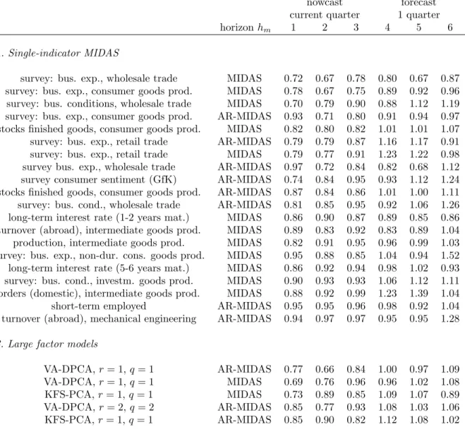
Now- and forecast results for the factor models and single-indicator MIDAS based on …xed speci…cations can be found in table 1. The table shows relative MSEs to the naive benchmark, which is the in-sample mean of GDP growth. The now- and forecasts are shown for monthly horizons hm = 1; : : : ;6, where horizons one to three belong to the
nowcast. Horizon hm = 1 is a nowcast made in the third month of the respective
quarter, whereas horizon hm = 2 is the nowcast made in the second month of the
current quarter. Thus, similar to standard forecast comparisons, increasing horizons correspond to less information available for now- and forecasting, and we expect an increasing MSE for increasing horizons hm. In the table, MSE results are shown for
selected MIDAS single-indicator models and factor models. To …nd the best-performing models in terms of MSE, we chose those with a relative MSE smaller than one for
hm = 1;2;3. To order the models, we use the average of the MSE overhm = 1;2;3.
In panel A of table 1, we …nd results concerning single-indicator MIDAS. We see that there are 20 models that have a relative MSE smaller than one up to hm = 3.
Regarding forecasts (hm = 4;5;6), only half of the models can consistently outperform
the naive benchmark, and in most of the cases only to a small extent. We do not report results for hm > 6, as the forecasts are almost always uninformative compared to the
benchmark. Among the top-performing models, surveys on business expectations play a big role, whereas industry statistics like incoming orders or turnover as well as interest rates play only a minor role. Concerning the MIDAS projections, both regressions with and without AR terms can be found among the best-performing models. Panel B of table 1 provides results for Factor-MIDAS. Here only 5 models yield relative MSEs consistently smaller than one for hm = 1;2;3. Regarding forecasts (hm = 4;5;6), the
factor models in most of the cases perform worse than the benchmark. Concerning the speci…cations, models with only one factor (r = q = 1) do best, and we …nd both MIDAS projections with and without AR terms in the ranking.
According to the results in table 1, factor models tend to perform worse than the best-performing single-indicator MIDAS models. However, in terms of the size of the MSE, the overall best-performing single-indicator model (survey: bus. exp., wholesale trade) and the best-performing factor model (VA-DPCA, r = 1, q = 1) seem to work similarly well for the nowcast, as the ranking of top models is changing over horizons. The results obtained so far are based on ex-post forecast MSEs only. Taking the
re-Table 1: Now- and forecast results for single-indicator MIDAS and factor models, MSE relative to in-sample mean forecast of GDP
nowcast forecast current quarter 1 quarter
horizonhm 1 2 3 4 5 6
A. Single-indicator MIDAS
survey: bus. exp., wholesale trade MIDAS 0.72 0.67 0.78 0.80 0.67 0.87 survey: bus. exp., consumer goods prod. MIDAS 0.78 0.67 0.75 0.89 0.92 0.96 survey: bus. conditions, wholesale trade MIDAS 0.70 0.79 0.90 0.88 1.12 1.19 survey: bus. exp., consumer goods prod. AR-MIDAS 0.93 0.71 0.80 0.91 0.94 0.97 stocks …nished goods, consumer goods prod. MIDAS 0.82 0.80 0.82 1.01 1.01 1.07 survey: bus. exp., retail trade AR-MIDAS 0.79 0.79 0.87 1.16 1.17 0.91 survey: bus. exp., retail trade MIDAS 0.79 0.77 0.91 1.23 1.22 0.98 survey bus. exp., wholesale trade AR-MIDAS 0.97 0.72 0.84 0.82 0.68 1.12 survey consumer sentiment (GfK) AR-MIDAS 0.74 0.84 0.95 0.93 1.12 1.24 stocks …nished goods, consumer goods prod. AR-MIDAS 0.87 0.84 0.86 1.01 1.00 1.11 survey: bus. cond., wholesale trade AR-MIDAS 0.81 0.85 0.95 0.92 1.06 1.26 long-term interest rate (1-2 years mat.) MIDAS 0.86 0.90 0.87 0.89 0.85 0.86 turnover (abroad), intermediate goods prod. MIDAS 0.89 0.83 0.92 0.83 0.89 1.04 production, intermediate goods prod. MIDAS 0.82 0.91 0.95 0.96 0.99 1.03 survey: bus. exp., non-dur. cons. goods prod. MIDAS 0.95 0.88 0.85 1.04 0.94 1.52 long-term interest rate (5-6 years mat.) MIDAS 0.86 0.92 0.94 0.98 1.02 0.93 survey: bus. cond., investm. goods prod. MIDAS 0.90 0.93 0.93 1.06 1.12 1.11 orders (domestic), intermediate goods prod. MIDAS 0.88 0.92 0.99 1.23 1.39 1.04 short-term employed AR-MIDAS 0.95 0.95 0.96 0.98 0.92 1.04 turnover (abroad), mechanical engineering AR-MIDAS 0.94 0.97 0.97 0.95 0.95 1.28
B. Large factor models
VA-DPCA,r= 1,q= 1 AR-MIDAS 0.77 0.66 0.84 1.00 0.97 1.09 VA-DPCA,r= 1,q= 1 MIDAS 0.69 0.76 0.96 0.96 1.02 1.08 KFS-PCA,r= 1, q= 1 MIDAS 0.73 0.89 0.85 1.09 1.07 0.89 VA-DPCA,r= 2,q= 2 AR-MIDAS 0.85 0.77 0.93 1.08 1.03 1.06 KFS-PCA,r= 1, q= 1 AR-MIDAS 0.85 0.90 0.82 1.12 1.08 1.02
Note: The entries in the table are relative MSEs relative to the in-sample mean, where the mean is recomputed every subsample. The model abbreviations in the …rst column are: VA-DPCA refers to the vertical realignment and dynamic PCA used in Altissimo et al. (2006), and KFS-PCA is the Kalman smoother of state-space factors according to Doz et al. (2006). The projection MIDAS-basic is the projection from Ghysels and Valkanov (2006), and AR-MIDAS is the basic MIDAS regression with an autoregressive term as proposed by Clements and Galvão (2007).
sults literally, the potential user of these methods could make use of the best-performing speci…cations. However, it is unclear whether the same results can be obtained in real-time also, when no a-priori knowledge about the best speci…cations is available to the practitioner. We consider this issue in the next subsection.
4.2
Information-criteria model selection and speci…cation based
on past performance
The …rst question we address in this subsection is whether we can …nd the best-performing speci…cations with in-sample information only. In particular, can we …nd the best-performing indicator variables for MIDAS and the optimal number of fac-tors without resorting on the ex-post forecast errors? The second question we ask is whether it is better to use model speci…cation based on information criteria or on the past forecasting performance.
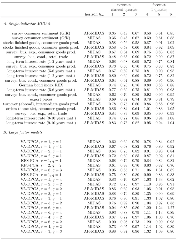
To address both questions, we will now compare the performance of …xed speci…ca-tions to time-varying speci…caspeci…ca-tions, where we use only information from the recursive subsamples to determine the model speci…cations. In table 2, we report the relative MSEs of the models speci…ed using information criteria and the past MSE performance, as described in subsection 3. In panel A of the table, we present the results based on Table 2: Now- and forecast results for single-indicator MIDAS and Factor-MIDAS, information criteria model selection, MSE relative to in-sample mean forecast of GDP
nowcast forecast current quarter 1 quarter
horizonhm 1 2 3 4 5 6
A. Information criteria model selection
single-indicator MIDAS/AR-MIDAS BIC 0.96 1.07 1.50 1.04 1.70 1.01 VA-DPCA, MIDAS Bai, Ng (2002, 2007) 1.09 1.00 0.95 1.19 1.35 1.08 VA-DPCA, AR-MIDAS Bai, Ng (2002, 2007) 1.17 0.84 0.83 1.28 1.05 0.77 KFS-PCA, MIDAS Bai, Ng (2002, 2007) 1.29 1.66 0.83 1.59 1.04 0.73 KFS-PCA, AR-MIDAS Bai, Ng (2002, 2007) 1.48 1.53 0.88 1.26 1.22 1.07
B. Model and variable selection by past MSE performance
single-indicator MIDAS MSE 0.86 1.26 0.99 1.20 1.05 1.24 large factor models MSE 0.89 0.84 0.85 0.93 0.91 0.66
Note: See table 1.
information-criteria model selection. When BIC is employed for selecting the predictor in MIDAS as well as the AR terms, we …nd only forhm = 1a relative MSE smaller than
the factor models, the information criteria also select speci…cations that perform worse than the benchmark for almost all the horizons with only a few exceptions. Panel B of table 2 contains the results with model speci…cation based on the past performance of the models in terms of MSE. For single-indicator MIDAS, where both AR terms as well as variable selection is done by BIC recursively, there is again only for hm = 1
a relative MSE smaller than one. The factor models, however, where the number of factors as well as AR terms are speci…ed using the past MSE, yield a good performance compared with the benchmark. For all horizons, the time-varying speci…cations yield relative MSEs smaller than one. Note that the factor model performance is for some of the horizons even better than the …xed speci…cations from the table 1. Therefore, the past performance seems to contain some information that can - in contrast to the …xed speci…cations over time - be exploited for now- and forecasting with factors.
If we compare the overall results from table 2 based on information criteria and performance-based model selection to the results with …xed speci…cations in table 1, the general impression is, that forecasting is much more di¢ cult when the model speci-…cations are unknown in pseudo real-time, as the relative MSEs in table 2 are generally larger than those in table 1. In particular, the information criteria applied to model selection lead to clearly inferior results. For example, without knowing the preferable predictor for MIDAS or the correct number of factors a priori, it is di¢ cult to specify these forecast models properly, and it is not possible to achieve the optimistic now-and forecast results from table 1. In this context, however, factor model speci…cation based on the past performance can still outperform the benchmark.
5
Nowcast pooling
After discussing the individual models’performance, we now assess nowcast pooling. As for information criteria and selection based on the past performance, pooling is only to a small extent subject to the data-mining critique, as only in-sample information is used to specify the weights.
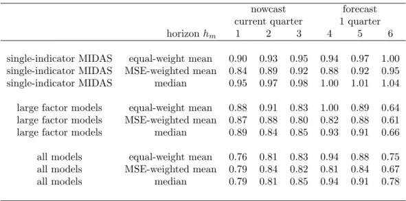
In table 3, we present now- and forecast results of the alternative pooling schemes described in section 2.3. The …rst three rows in the table contain the results when all the single-indicator MIDAS now- and forecasts are combined using equally weighted mean, MSE-based mean as well as the median. The results indicate an information content for both the nowcast and the forecast one quarter ahead, as the relative MSEs are smaller than one in many cases.2 Concerning the pooling methods, the median
tends to perform worse than the unweighted mean, and both are outperformed by the MSE-based weighted mean. Compared with …gures based on model selection from table 2, the results are now clearly better, indicating advantages of pooling over model
2Note that results for larger horizonsh
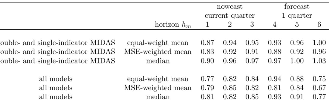
Table 3: Now- and forecast results for nowcast pooling, MSE relative to in-sample mean forecast of GDP
nowcast forecast current quarter 1 quarter
horizonhm 1 2 3 4 5 6
single-indicator MIDAS equal-weight mean 0.90 0.93 0.95 0.94 0.97 1.00 single-indicator MIDAS MSE-weighted mean 0.84 0.89 0.92 0.88 0.92 0.95 single-indicator MIDAS median 0.95 0.97 0.98 1.00 1.01 1.04 large factor models equal-weight mean 0.88 0.91 0.83 1.00 0.89 0.64 large factor models MSE-weighted mean 0.87 0.88 0.80 0.82 0.88 0.61 large factor models median 0.89 0.84 0.85 0.93 0.91 0.66 all models equal-weight mean 0.76 0.81 0.83 0.94 0.88 0.75 all models MSE-weighted mean 0.79 0.84 0.82 0.81 0.84 0.67 all models median 0.79 0.81 0.85 0.94 0.91 0.78
Note: See table 1.
selection. Rows four to six contain results from pooling all the factor models that di¤er with respect to the number of factors and the AR term in the Factor-MIDAS projection. The results are again better than those based on model selection from table 2, and the MSE-based weighted mean outperforms the other weighting schemes for most of the horizons, although the di¤erences are smaller than in the case of single-indicator MIDAS. Comparing the levels of relative MSEs between factor models and single-indicator MIDAS, we …nd a slightly better performance of the factor combinations.
The …nal three rows contain now- and forecast combinations of all the models under consideration. Here, the ranking of the di¤erent pooling methods is less clear. The interesting result is that the combination of all forecast models provides overall smaller relative MSEs than the combinations of factor and single-indicator MIDAS alone. Thus, taking into account model uncertainty to a wider extent than just pooling within a model class seems to improve the forecasting performance. Furthermore, pooling over all models almost entirely outperforms the individual models chosen by information criteria or the past performance in table 2.
But what about the performance compared to the …xed speci…cations in table 1? Is nowcast pooling also competitive to the ex-post best-performing models? A direct comparison of tables 1 and 3 suggests that even pooling cannot perform as well as the ex-post best performing models, though the di¤erences are often small.
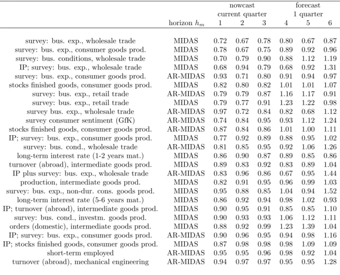
In order to analyze this issue in more details, we investigate the relationship between the groups of individual models and the forecast combinations. For this purpose, we present percentiles of the relative MSEs from the alternative nowcast pools for each horizon. The percentiles provide an indication of how the pooling MSE values compare
to those of the individual models. Table 4 contains the results. The entries in the table Table 4: Percentiles of the MSEs from now- and forecast pooling in the cumulative distribution of individual models
nowcast forecast current quarter 1 quarter
horizonhm 1 2 3 4 5 6
A. Pooling vs single-indicator MIDAS
MIDAS models equal-weight mean 0.13 0.16 0.15 0.13 0.21 0.22 MIDAS models MSE-weighted mean 0.08 0.11 0.10 0.07 0.11 0.13 MIDAS models median 0.23 0.22 0.21 0.26 0.31 0.29 all models equal-weight mean 0.03 0.04 0.02 0.13 0.07 0.02 all models MSE-weighted mean 0.05 0.07 0.02 0.02 0.04 0.00 all models median 0.05 0.04 0.03 0.13 0.10 0.02
B. Pooling vs individual large factor models
large factor models equal-weight mean 0.25 0.22 0.11 0.20 0.06 0.08 large factor models MSE-weighted mean 0.24 0.17 0.06 0.00 0.06 0.06 large factor models median 0.25 0.14 0.13 0.06 0.07 0.10 all models equal-weight mean 0.07 0.12 0.11 0.09 0.06 0.21 all models MSE-weighted mean 0.12 0.14 0.08 0.00 0.04 0.10 all models median 0.11 0.12 0.13 0.08 0.07 0.24
Note: The entries in the table can be interpeted as follows. An entryximplies that the MSE of the combination of single-indicator MIDAS models is larger than 100 x percent of the MSEs of the individual MIDAS models, and accordingly smaller than100 (1 x) percent of the MSEs from the worse-performing models. Thus, the pool is in the(100 x)th percentile of the distribution of individual models. In the table, the model set used in the combination of now- and forecasts can be found in the …rst column of the table. The second column contains the weighting methods employed.
can be interpreted as follows. In panel A of table 4, entry 0:13 for hm = 1 implies
that the MSE of the combination of single-indicator MIDAS models is larger than 13 percent of the MSEs of the individual MIDAS models, and accordingly smaller than87 percent of the MSEs from the worse-performing models. Thus, the pool is in the 13th percentile of the distribution of individual models. The results in table 4 con…rm that nowcast pooling is in almost all of the cases not the best-performing method. However, based on the MSE-weighted mean for all horizons reported, the pool is between the 7th and 13th percentile compared to the individual single-indicator MIDAS models (row 2). Combining factor models and single-indicator MIDAS reduces the relative MSE further, and the pooled forecast ends up in the 7th percentile and lower (row 5). The best combinations can outperform between 93 and 100 percent of the individual MIDAS models, depending on the forecast horizon.
Looking at the distribution of factor models in panel B, we …nd that pooling of the factor models only using the MSE-weighted mean is doing better than76to94percent