A Dissertation by
CHANGWOO NAM
Submitted to the Office of Graduate Studies of Texas A&M University
in partial fulfillment of the requirements for the degree of DOCTOR OF PHILOSOPHY
August 2011
A Dissertation by
CHANGWOO NAM
Submitted to the Office of Graduate Studies of Texas A&M University
in partial fulfillment of the requirements for the degree of DOCTOR OF PHILOSOPHY
Approved by:
Chair of Committee, Hwagyun Kim Committee Members, Neal Galpin
Ryo Jinnai Qi Li
Head of Department, Timothy Gronberg
August 2011
ABSTRACT
Essays on A Rational Expectations Model of Dividend Policy and Stock Returns. (August 2011)
Changwoo Nam, B.A., Sung Kyun Kwan University;
M.A., Seoul National University; M.S., The University of Texas at Austin Chair of Advisory Committee: Dr. Hwagyun Kim
We propose an asset pricing model in a production economy where cash flows are determined by firms’ optimal dividend and investment decisions. Extensive and tensive decision margins in dividend payout are modeled with cash holding and in-vestment adjustment costs. The model implies that delays in dividend distribution of young and growing firms play instrumental roles in explaining various asset pric-ing anomalies. Quantitative results show that model-implied dividend policies and investments are consistent with data, and the cross sections of stock returns are well explained by the interactions between productivity shocks and the lumpy dividend policies. Additionally, the model produces countercyclical variations in the market risk premium.
In addition, we empirically investigate the relevance of firm characteristics and aggregate productivity shocks in determining dividend payment propensity, thereby asset prices. It is found that excess returns for dividend payers over nonpayers are significantly linked to business cycles. Relative future returns are fairly predicted by the spread of lagged propensities to pay dividends. Furthermore, the empirical results document that each future return of payers and nonpayers increases in propensities to pay out cash to shareholders. These results are consistent to our rational expectations model of dividend policy, and contradictory to the catering theory of dividends.
ACKNOWLEDGMENTS
I am happy to have this opportunity to express my gratitude to those who helped to make this dissertation possible. Without these people’s love, support and dedication, I might not have been able to finish this long and demanding journey of doctoral studies.
I would like to express my deepest gratitude to my advisor, Dr. Hwagyun Kim, who has consistently encouraged, motivated and guided me through the dissertation process. He has been a thoughtful mentor and a great role model. I would like to extend my gratitude to my committee members, Dr. Neal Galpin, Dr. Ryo Jinnai, and Dr. Qi Li, for their insightful feedback and valuable suggestions that have broadened my knowledge and enriched my work. I specially thank Dr. Galpin and Dr. Jinnai for directing me to readings of particular importance to this study, and for helpful comments on each chapter.
I would like to thank my parents, Sangkil Nam and Sungja Lee. They have always supported me. My parents-in-law, Chunsik Lee and Mijung Kim, have encouraged me with their best wishes. Finally, I want to thank my wife, Hyunju Lee. She has always been there to cheer me up and to stand by me through the good times and the bad. I love you.
TABLE OF CONTENTS
CHAPTER Page
I INTRODUCTION. . . 1
II TO PAY OR NOT TO PAY: A DIVIDEND-BASED EX-PLANATION OF ASSET PRICING ANOMALIES . . . 7
A. Introduction . . . 7
B. Model . . . 12
1. Individual Firm Dynamics . . . 12
2. Preferences and Asset Prices . . . 19
3. Equilibrium . . . 22
C. Cross Sections of Stock Returns . . . 23
1. The Value Premium . . . 24
2. The Size Premium . . . 27
D. Quantitative Analysis . . . 29
1. Calibration . . . 29
2. Investment, Dividend Policy, and Cash Holdings . . . 32
3. Analyzing Stock Returns . . . 34
a. Aggregate Market Values . . . 35
b. Conditional Risk Premiums and Betas . . . 37
c. Cross-Sectional Analysis of Stock Returns . . . . 39
E. Conclusion . . . 42
III DIVIDEND PAYMENT PROPENSITY, BUSINESS CYCLES AND STOCK RETURNS . . . 44
A. Introduction . . . 44
B. Testable Hypotheses . . . 46
C. Empirical Analysis . . . 48
1. Data Variables for Empirical Analysis . . . 48
2. Empirical Tests for Testable Hypotheses . . . 53
D. Conclusions . . . 56
IV CONCLUSION . . . 58
CHAPTER Page
APPENDIX A . . . 65
APPENDIX B . . . 73
APPENDIX C . . . 76
LIST OF TABLES
TABLE Page
I Benchmark Parameter Value Sets . . . 76 II Unconditional Moments of Market Values . . . 77 III Size and Value Factors and the Size-BE/M E Portfolios . . . 78 IV Logit Regressions of Propensities of Payouts: Dividend Payment
and Stock Repurchase, 1962 to 2009 . . . 79 V Statistics for Measures of Payout: Dividend Payment and Stock
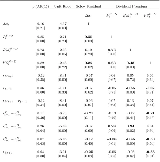
Repurchase, Solow Residual and Dividend Measures, 1962 to 2009 . . 80 VI Statistics for Solow Residual, Demand for Dividend Measures and
Stock Returns, 1962 to 2009 . . . 81 VII Measures of Payout: Dividend Payment and Stock Repurchase
and Stock Returns, 1962 to 2009 . . . 82 VIII Regressions of Stock Returns on Measures of Payout: Dividend
LIST OF FIGURES
FIGURE Page
1 Lumpy Dividend Policies. . . 85
2 Aggregate Payout Ratios. . . 86
3 Non-convex Managerial Cost: Π + Ξ . . . 87
4 V0 and V1 according to Increase in x . . . 88
5 The Optimal Policy Functions Givenxt: Model M . . . 89
6 The Optimal Policy Functions Givenzt: Model M . . . 90
7 The Optimal Policy Functions Givenxt: Model Q. . . 91
8 The Optimal Policy Functions Givenzt: Model Q . . . 92
9 Countercyclical Time-Varying Risks . . . 93
10 Conditional Expected Market Returns andβM . . . 94
11 Time-Varying VMG and Value Spread in Quarterly Frequency . . . . 95
12 Expected Returns on 10 Portfolios Formed onBE/M E and Mar-ket Size . . . 96
13 Solow Residual and Dividend Premiums, 1962 to 2009 . . . 97
14 Propensities of Payouts: Dividend Payment and Stock Repur-chase, 1962 to 2009 . . . 98
CHAPTER I
INTRODUCTION
It is well known that corporate decisions made by firm managers matter in explaining the cross-sectional properties of stock returns. Especially, if decisions on investment and dividend payout can affect cash flows of firms, these have direct implications on the equity prices of firms, since the cash flow processes of firms are one of the two main pillars determining stock prices. The other pillar, stochastic discount factor, is closely related to the changes of market investor’s wealth given their attitudes toward risk and uncertainty. Since the distributed cash flows of firms will constitute the current and future wealths of market investors, corporate financial decisions related to investments and dividends can have important links to variations in asset prices via channels of both firms’ cash flows and investors’ discount factors. This paper studies the implications of corporate dividend policies on stock returns in a general equilibrium framework.
We develop a dynamic general equilibrium model of asset prices with many firms whose dividend processes are endogenously determined by firms’ optimal dividend policies and investment behaviors. In so doing, both extensive and intensive deci-sion margins in dividend payout are modeled. Corporate managers will maximize the present value of current and future cash flows net of dividends and the costs in-volved with investment and cash holding. Cash holding is assumed costly to reflect the agency cost or the conflict of interests between shareholders and firm managers. Easterbrook (1984) and Jensen (1986) are the classic studies suggesting that firm
managers pursue self-interests, and increase cash holdings for various reasons. In this case, they argue that dividends can help shareholders to reduce the associated agency costs. Recently, Nikolov and Whited (2009) estimate a dynamic model of firm investment and cash accumulation to find that agency problems affect corporate cash holding decisions. They model three specific mechanisms that misalign managerial and shareholder incentives: managerial bonuses on current profits, limited managerial ownership of the firm, and a managerial preference for firm size. Our setup can be viewed as an attempt to incorporate these findings in the corporate finance into a general equilibrium framework.
The model features rich firm dynamics and generates several cross-sectional im-plications of asset returns and firm characteristics. Regarding the firm dynamics, both analytic and quantitative results show that younger firms with small capital tend to invest more in capital, and they withhold paying dividends. These firms ini-tiate dividend payouts mainly to reduce the increasing cash holding and investment costs, as capital is accumulated. It turns out that this extensive decision margin on firm cash flow depends on firm characteristics associated with productivity shocks.1 Thus, this model endogenizes not only the amount but also the timing of cash flows distributed from firms to shareholders. Note that the latter is reminiscent of duration-based explanations of the value premium examined by Lettau and Wachter (2007) and Santos and Veronesi (2010). These papers view that growth stocks pay later, while value firms pay now. Alas, if there exist long-run risks (persistent shocks in economic growth, for instance) in an economy and the discount factor co-varies with 1These theoretical findings are consistent with the firm life cycle theory of divi-dends. For more details, see Mueller (1972), Grullon, Michealy, and Swaminathan (2002), DeAngelo, DeAngelo, and Skinner (2004), DeAngelo, DeAngelo, and Stulz (2006). On the firm characteristics for the propensity to pay dividends, see Fama and French (2001) and Denis and Osobov (2008).
stock prices, counterfactual growth premiums can occur. To overcome this, Lettau and Wachter (2007) assume that shocks to the discount factor do not co-vary with cash flows shocks, and Santos and Veronesi (2010) assume that cash flows are highly volatile. The former is difficult to justify in an equilibrium, while the latter needs an abnormal amount of cash flow fluctuations. In our model, young and growing firms typically do not pay dividends, and therefore covariations with the discount factor are close to zero. Meanwhile mature firms with larger amounts of capital pay dividends, and tend to have less room for growth. Thus, their short-run cash flows become risky and accordingly priced. In this vein, our paper provides a novel explanation of the value premium which extends and generalizes the insight from the durations of assets based on firms’ cash flows.2
With this model in hand, we analyze the behaviors of stock returns generated from the simulated cash flows of firms. According to our quantitative results, the expected returns on value and size sorted portfolios are consistent with the historical data (e.g., Fama and French (2007) and Chen, Petkova, and Zhang (2008)). In addition, the simulated expected returns on decile portfolios sorted by book-to-market equity ratio and size present features of value and size premia in the empirical facts (Fama and French (1992)). Interestingly, pooling new decile portfolios sorted by fitted propensity to pay dividends, the simulated expected returns on them consistently increase in the likelihood of dividend payout. This implies that the factors affecting dividend policy largely overlap with the characteristics used to form pricing factors. Finally, the simulated market risk premiums and volatilities of aggregate dividend and asset returns reveal endogenously countercyclical variations, again in line with empirical evidence.
2The size premium can also arise due to the delay in dividend payout and the profitability of firms in this model.
Our work also belongs to another line of literature on the asset pricing model, which extends Lucas (1978) to have many trees (dividends). Cochrane, Longstaff, and Santa-Clara (2008) solve a model with two Lucas trees. They show that ex-pected returns, excess returns, and return volatility as functions of dividend share vary through time, and returns are predictable from price-dividend ratios. Mar-tin (2009) further extends Cochrane, Longstaff, and Santa-Clara (2008) with many trees. Menzly, Santos, and Veronesi (2004) propose a general equilibrium model with multiple securities in which investors’ risk preferences, and expectations of dividend growth are time-varying with external habit formation. Santos and Veronesi (2010) show that substantial heterogeneity in firm’s cash-flow risk yields both a value pre-mium as well as most of the stylized facts about the cross-section of stock returns, but it generates a “cash-flow risk puzzle”. All these papers assume exogenous pro-cesses for dividend propro-cesses. Therefore, these papers are restrictive in linking firm characteristics to asset prices. In this context, our paper can be viewed as a general equilibrium justification of Lucas models with multiple trees.
In addition, we empirically investigate the relevance of firm characteristics and aggregate productivity shocks in determining dividend payment propensity and stock returns, and we analyze the implications of serial correlations of stock returns. Our rational expectations model of dividend policy shows that differences in dividend poli-cies result from firm characteristics including the level of firm maturity and variations in aggregate productivity shocks, and dividend policy, especially in extensive margin can affect stock returns via shifting cash flows of firms. We further show that this channel can explain some major asset pricing anomalies such as the value and size premia. Therefore, without resorting to the existence of irrational investors such as the catering theory of dividends (Baker and Wurgler (2004b)), it is possible to link stock returns and propensity to pay dividends. Especially, we have shown that the
propensity to pay dividend (PPD, hereafter) is positively related to the future stock returns since the cash flow risk is definitely linked to the probability of dividend payment in the next period and the cumulated cash flow risks in discount risk effect (long-term dividend growth rate) must be associated to conditional PPDs. Therefore, once we can appropriately find the proxy (fitted PPD by logit regression, Fama and French (2001)) for the probability of dividend payment or payout, then it is possi-ble to scrutinize the predictability of relative returns of dividend-payers’ stocks and nonpayers’ stocks, payout stocks and nonpayout stocks (including stock repurchase). The important issue is the comparison of rational expectations model and be-havioral asset pricing model. Baker and Wurgler (2004b) posit that the decision on paying dividends is made by prevailing investor demand for dividend payers. In other words, investors prefer dividend-paying firms because they ignore some cost of excess dividends to long-run growth of firms and rational firm mangers respond to this excess demand up to some costs. This makes dividend premium exist and related to dividend payment decisions. This so-called catering theory of dividend payment emphasizes the roles of stock mispricing in explaining the relationship between dividend policy and stock returns. The casual intuition suggests that the dividend premium and ini-tiation effects are positively related to excess demand for payers. However, they find that the difference in future returns of payers and nonpayers is negatively related to this demand in empirical analysis because overpricing stocks by excess supply of div-idends makes payers’ future returns relatively low. But, by our rational expectations model of dividend policy, the relative returns of payers and nonpayers are explained by PPDs dependent on business cycles, not by mispricing stocks. Especially, we show that these relative returns are countercyclical due to the time-varying differences be-tween rational investors’ risk premiums for dividend payers and nonpayers, or payouts and non-payouts. In addition, the empirical results document that each future return
of payers and nonpayers is positively correlated to propensities of paying out cash. These results are consistent to our rational model of payout policies, but contradict the catering theory of dividend because according to their security overpricing, future returns should have been negatively linked to propensities and measures of dividend payment.
CHAPTER II
TO PAY OR NOT TO PAY: A DIVIDEND-BASED EXPLANATION OF ASSET PRICING ANOMALIES
A. Introduction
Do corporate decisions made by firm managers matter in explaining the cross-sectional properties of stock returns? Especially, if decisions on investment and dividend payout can affect cash flows of firms, these have direct implications on the equity prices of firms, since the cash flow processes of firms are one of the two main pillars determining stock prices. The other pillar, stochastic discount factor, is closely related to the changes of market investor’s wealth given their attitudes toward risk and uncertainty. Since the distributed cash flows of firms will constitute the current and future wealths of market investors, corporate financial decisions related to investments and dividends can have important links to variations in asset prices via channels of both firms’ cash flows and investors’ discount factors. This paper studies the implications of corporate dividend policies on stock returns in a general equilibrium framework.
There are several studies that attempt to connect the investment and production behaviors of firms to stock returns (e.g., Cochrane (1996), Gomes, Kogan, and Zhang (2003), Zhang (2005), Li, Livdan, and Zhang (2009), and Livdan, Sapriza, and Zhang (2009)). However, the existing literature pays little attention to dividend policy, and the authors assume that dividends are given as residual cash flow. Simple as it may be, the assumption of this residual dividend policy is not consistent with empirical evidence. Figure 1 plots earnings per share and dividends per share of several firms. Dividends appear to be managed with the following patterns: First, there are periods of no dividend payments which make earnings much more volatile,
and second, dividends and earnings share a common trend over time, though the latter more volatile, other than the period of zero dividends.1 Thus, modeling whether and when to pay dividends seems relevant in describing dividend policy.
Empirical studies report that highly related are the extensive/intensive margins of dividend payout and key firm characteristics frequently used in empirical asset pricing studies. Fama and French (2001) find that four characteristics have effects on the decision to pay dividends: profitability, investment opportunities, market-to-book ratio, and size. Larger and more profitable firms are more likely to pay dividends, and paying dividends is less likely for firms with more investments. Grullon, Michealy, and Swaminathan (2002) report that the firm profitability declines after a dividend increase and rises after a dividend decrease. DeAngelo, DeAngelo, and Stulz (2006) present evidence that the probability that a firm pays dividends is significantly related to the mix of earned capital and contributed capital in its capital structure. Firms with a greater proportion of earned capital are more likely to be dividend payers. Bulan, Subramanian, and Tanlu (2007) use duration analysis to study the timing of dividend initiations in a firm’s life cycle, and document that firms initiate dividends after reaching the maturity phase in their life cycles. Putting together, initiators are the firms that have grown larger and have fewer growth opportunities than do non-payers at the same stage in their life cycles.
Based on these observations, we develop a dynamic general equilibrium model of asset prices with many firms whose dividend processes are endogenously determined by firms’ optimal dividend policies and investment behaviors. In so doing, both ex-tensive and inex-tensive decision margins in dividend payout are modeled. Corporate 1It is well known that, at the aggregate level, dividend payments tend to be smooth relative to earnings, suggesting that corporate managers manage dividends (Lease, John, Kalay, Lowenstein, and Sarig (1999)).
managers will maximize the present value of current and future cash flows net of dividends and the costs involved with investment and cash holding. Cash holding is assumed costly to reflect the agency cost or the conflict of interests between share-holders and firm managers. Easterbrook (1984) and Jensen (1986) are the classic studies suggesting that firm managers pursue self-interests, and increase cash hold-ings for various reasons. In this case, they argue that dividends can help shareholders to reduce the associated agency costs. Recently, Nikolov and Whited (2009) estimate a dynamic model of firm investment and cash accumulation to find that agency prob-lems affect corporate cash holding decisions. They model three specific mechanisms that misalign managerial and shareholder incentives: managerial bonuses on current profits, limited managerial ownership of the firm, and a managerial preference for firm size. Our setup can be viewed as an attempt to incorporate these findings in the corporate finance into a general equilibrium framework.
The model features rich firm dynamics and generates several cross-sectional im-plications of asset returns and firm characteristics. Regarding the firm dynamics, both analytic and quantitative results show that younger firms with small capital tend to invest more in capital, and they withhold paying dividends. These firms ini-tiate dividend payouts mainly to reduce the increasing cash holding and investment costs, as capital is accumulated. It turns out that this extensive decision margin on firm cash flow depends on firm characteristics associated with productivity shocks.2 Thus, this model endogenizes not only the amount but also the timing of cash flows distributed from firms to shareholders. Note that the latter is reminiscent of duration-2These theoretical findings are consistent with the firm life cycle theory of divi-dends. For more details, see Mueller (1972), Grullon, Michealy, and Swaminathan (2002), DeAngelo, DeAngelo, and Skinner (2004), DeAngelo, DeAngelo, and Stulz (2006). On the firm characteristics for the propensity to pay dividends, see Fama and French (2001) and Denis and Osobov (2008).
based explanations of the value premium examined by Lettau and Wachter (2007) and Santos and Veronesi (2010). These papers view that growth stocks pay later, while value firms pay now. Alas, if there exist long-run risks (persistent shocks in economic growth, for instance) in an economy and the discount factor co-varies with stock prices, counterfactual growth premiums can occur. To overcome this, Lettau and Wachter (2007) assume that shocks to the discount factor do not co-vary with cash flows shocks, and Santos and Veronesi (2010) assume that cash flows are highly volatile. The former is difficult to justify in an equilibrium, while the latter needs an abnormal amount of cash flow fluctuations. In our model, young and growing firms typically do not pay dividends, and therefore covariations with the discount factor are close to zero. Meanwhile mature firms with larger amounts of capital pay dividends, and tend to have less room for growth. Thus, their short-run cash flows become risky and accordingly priced. In this vein, our paper provides a novel explanation of the value premium which extends and generalizes the insight from the durations of assets based on firms’ cash flows.3
With this model in hand, we analyze the behaviors of stock returns generated from the simulated cash flows of firms. According to our quantitative results, the expected returns on value and size sorted portfolios are consistent with the historical data (e.g., Fama and French (2007) and Chen, Petkova, and Zhang (2008)). In addition, the simulated expected returns on decile portfolios sorted by book-to-market equity ratio and size present features of value and size premia in the empirical facts (Fama and French (1992)). Interestingly, pooling new decile portfolios sorted by fitted propensity to pay dividends, the simulated expected returns on them consistently increase in the likelihood of dividend payout. This implies that the factors affecting 3The size premium can also arise due to the delay in dividend payout and the profitability of firms in this model.
dividend policy largely overlap with the characteristics used to form pricing factors. Finally, the simulated market risk premiums and volatilities of aggregate dividend and asset returns reveal endogenously countercyclical variations, again in line with empirical evidence.
This paper is related to growing literature that links the cross-sectional properties of stock returns to firm characteristics. Gomes, Kogan, and Zhang (2003) construct a dynamic general equilibrium production economy to explicitly link expected stock returns to firm characteristics such as the firm size and the book-to-market equity ratio. Zhang (2005) shows that the value premium occurs from the asymmetric cost of reversibility and the countercyclical price of risk, and assets in place are riskier than growth options especially in bad times when the price of risk is high. Li, Livdan, and Zhang (2009) use a simpleq-theory model, and ask if it can explain external financing anomalies, both qualitatively and quantitatively. Livdan, Sapriza, and Zhang (2009) analyze the effect of financial constraints on risk and expected returns by extending the investment-based asset pricing framework to incorporate retained earnings, debt, costly equity, and collateral constraints on debt capacity. However, this paper differs from all these studies in that our model explains the cross section of stock returns using endogenous dividend policies as well as production and investment. As men-tioned earlier, models missing this feature can have counterfactual implications on the relationships between stock returns and firm characteristics.
Our work also belongs to another line of literature on the asset pricing model, which extends Lucas (1978) to have many trees (dividends). Cochrane, Longstaff, and Santa-Clara (2008) solve a model with two Lucas trees. They show that ex-pected returns, excess returns, and return volatility as functions of dividend share vary through time, and returns are predictable from price-dividend ratios. Mar-tin (2009) further extends Cochrane, Longstaff, and Santa-Clara (2008) with many
trees. Menzly, Santos, and Veronesi (2004) propose a general equilibrium model with multiple securities in which investors’ risk preferences, and expectations of dividend growth are time-varying with external habit formation. Santos and Veronesi (2010) show that substantial heterogeneity in firm’s cash-flow risk yields both a value pre-mium as well as most of the stylized facts about the cross-section of stock returns, but it generates a “cash-flow risk puzzle”. All these papers assume exogenous pro-cesses for dividend propro-cesses. Therefore, these papers are restrictive in linking firm characteristics to asset prices. In this context, our paper can be viewed as a general equilibrium justification of Lucas models with multiple trees.
The outline for the rest of this chapter is as follows: The recursive competitive equilibrium with dynamic problems is described in Section B, and our theoretical findings about the firm characteristics and the cross-section of stock returns are ex-plored in Section C. Section D outlines the quantitative analysis of cross-sectional stock returns including the baseline calibration, and discusses the consistency of our findings related to similar literature. Finally, Section E concludes.
B. Model
1. Individual Firm Dynamics
This section sets up the dynamic and stochastic problem of firms. The economy is composed of a continuum of competitive firms that produce a homogeneous prod-uct. Firms are subject to an aggregate productivity shock (xt) and a firm-specific productivity shock (zit)4. The aggregate shock, xt, develops according to a
first-order autoregressive stationary and monotone Markov transition function, denoted 4This convention is based on recent macro-finance literature: Zhang (2005), Li, Livdan, and Zhang (2009), and Livdan, Sapriza, and Zhang (2009).
bydQx(xt+1|xt),
xt+1 =µx(1−ρx) +ρxxt+xt+1,
in whichx follows truncatedN(0, σx2), and xtserves as the driving force of economic
fluctuations and systematic risks. xt has the finite support as [x,x¯]. Similarly, the
firm specific productivity shocks,{zit}i∈[0,1]withdQz(zit+1|zit) are uncorrelated across
firms, and follow
zit+1 =ρzzit+it+1,
in which i follows truncated N(0, σz2), and xt+1 is independent of it+1 for all i. zit
has the finite support as [z,z¯].
The production function is given by
yit =ezit+xtKitθ,
in whichKit is the capital of firmiat timet,and has the compact support ofK,K¯. The assumption on capital implies that firms have limited investment opportunities as firms accumulate capital close to the upper bound. The production function ex-hibits decreasing returns to scale: the curvature parameter satisfies 0< θ <1. The operating profit is, then, defined as,
Π (Kit, xt, zit) = ezit+xtKitθ −f,
in whichf is the nonnegative fixed production cost, which is paid in every period5. With this production technology in hand, we now describe the firm’s decision process below. In the beginning of period t, firm i observes current aggregate and firm-specific shocks. Then, it decides whether to pay dividends to shareholders (ait =
5For mathematical simplicity, we assume that f is zero in driving our theoretical results.
1 : paying dividends, ait = 0 : not-paying dividends). In particular, the dividend
payment (Dit) is determined by a fixed payout ratio 0 < δ <1 as
(2.1) Dit=aitδΠ (Kit, xt, zit) =aitδezit+xtKitθ.
To motivate our choice of dividend policy dictated by (2.1), we plot Figure 1. As mentioned earlier, Figure 1 illustrates the existence of zero dividend periods for in-dividual firms. Although we do not tabulate here, a significant number of firms do not pay dividends at any given point of time. Thus, we believe that it is pertinent to include the discrete decision of dividend distribution. In addition, this figure suggests that dividend and corporate earnings follow a common trend, excluding the period of no dividend, which makes (2.1) a reasonable approximation of reality. We further investigate this issue in Figure 2. Panel (A) in Figure 2 displays the aggregate payout ratios in the U.S. stock market during 1950 and 2009. Although there exist some variations, the payout ratio is stable around 0.5. To see if the variations result from the usual suspects such as profitability and investments, we run rolling regressions of the aggregate payout ratio onto those variables. We find that both variables are mostly not different from zero, and the negative sign of the profitability is inconsistent with the related theory.
After the decision of paying dividends, the firm manager of firm i chooses the optimal investmentIa
it to maximize the present value of future cash streams under the
operating profit less dividends. This cash accumulation decision is motivated from the empirical findings in the corporate finance literature6. Related, firms often need to hold a significant amount of funds (cash and marketable securities) to allow for future 6For instance, Nikolov and Whited (2009) argues that although numerous empiri-cal researchers have studied the effects of agency conflicts on cash holding, this topic remains of interest because no single prominent conclusion has emerged from these exercises.
acquisitions and to cover its considerable legal and business risks (Harford (1999)).7 It is also well known that there exists an agency conflict between managers and equity providers, and increasing cash holdings further intensify this type of agency problem.8 That is, increasing the cash holdings of firms is a costly business. Incorporating this stylized fact, we set up a firm’s dynamic decision problem with a non-convex agency cost function in the following way.
Vi(Sit) = max {ait=0,ait=1} Vait i (Sit) for all (Kit, xt, zit)≡Sit ∈ S, (2.2) Vait i (Sit) = max Ia it {vait−Ξ (vita, Kit, xt, zit) +βEt[Vi(Sit+1)|Sit]},
in whichVait=0 is the present value of future cash streams reserved when it does not
pay dividends, Vait=1 is the present value of future cash flows held by a firm paying
dividends,va
itis the current cash held and used by the firm manager before the cost of
reserving the cash, Ξ (va
it, Kit, xt, zit) is the cash holding cost, S is a compact product
space of state variables, andEt is the expectation operator at timet.9 Thus, the firm imaximizes the present value of the net cash flows into the corporate cash holdings, defined asvait
it −Ξ(v ait
it , Kit, xt, zit) with the decision of paying or not paying dividends
7From the perspective of corporate governance, Harford (1999) states that cash is an important tool for firms operating in imperfect capital markets. However, firms of-ten build up much more cash than they need to meet expected financing requirement, which also provides another rational on why managers accumulate cash reserves, and it is subject to a source of agency cost. Harford, Mansi, and Maxwell (2008) find that firms with weaker corporate governance structures actually have smaller cash reserves, and weakly controlled managers tend to spend cash quickly on acquisitions and capital expenditures.
8Readers are referred to Jensen and Meckling (1976), Jensen (1986), Easterbrook (1984) for more on this issue.
9The superscript a is sometimes suppressed, when it is not confusing, for the purpose of expositional ease. For instance, when we integrate over i, we will simply use vit instead ofvita.
each period as well as an investment decision.10 Furthermore, we define vita as
vait≡Π (Kit, zit, xt)−Dit−Φ (Iita, Kit),
and Φ (I, K)≡ φ 2 I K 2 K +I,
in which Φ is a quadratic investment adjustment cost with a constant φ >0. Regarding the cash holding cost, Ξ (vait
it , Kit, xt, zit), we assume the following
quadratic form: Ξ (v, K, x, z)≡ ξ1e ξ2(x+z) 2 v K 2 K,
in which ξ1, ξ2 > 0 are constant parameters. This reflects the idea that sharehold-ers would expect more dividends to be paid in good times, and increasing the cash holdings of firms becomes more costly. The law of motion for capital is expressed as
Kit+1 =Iita + 1−δ¯
Kit,
in which ¯δ is a constant depreciation rate of capital stocks. This setup allows that capital in the next period may depend upon dividend policy, especially around the time of initiating dividend payment, since whether a firm pays a proportion of cash flow from the profit as dividend to a shareholder determines the amount of investment given the investment opportunity set.
Recall that firm managers are subject to costs due to the agency problem men-tioned above. This not only has a direct implication on the payout policy of firms, but also affects firms’ capital accumulation paths over time. Furthermore, note that the total cost defined as Φ + Ξ is state-dependent, depending on the firms’ choices 10We can define a felicity function for firm manager,F such that her periodic utility is F(vita −Ξ (vita, Kit, xt, zit)), where F0 > 0, and F00 ≤ 0. In this context, our setup assumes that firm managers are risk-neutral.
of extensive margins on the dividend payout. Specifically, even if each of Φ and Ξ is a convex function, total cost function is non-convex in investment. Figure 3 displays this feature. Notice that the level of investment corresponding to the minimum cost of non dividend payment, (Φ0+ Ξ0) is bigger than that of the minimum cost when paying dividend, (Φ1+ Ξ1). This property results from the fact that dividend pay-ment effectively reduces the range of possible investpay-ments by lowering down cash flow in hand. In addition, the total cost function shifts to the right as capital increases. Once a firm has enough cash in hand and fewer marginal profitable investment op-tions, it has the incentive to pay dividends to reduce the cash holding cost as well as the investment adjustment cost.
The recursive problem of firm (2.2) is well defined, and the existence of a solution can be easily established, summarized in the following proposition.
Proposition II.1. There exists a solution to the functional equation (2.2).
Proof. We refer to Theorem 9.6 in Stokey and Lucas (1989).
Now we characterize the firm dynamics implied by our model. In light of optimal dividend policy, the probability of paying dividends is described as
P{a= 1|S}= 1
if and only if V1 > V0 given the state vector S ∈ S. In this context, the propensity to pay dividends (PPD, hereinafter) following Fama and French (2001) is defined as, (2.3) P{at+u = 1|St} ≡
Z
S
at+udQ(St+u|St),
in which dQ is the transition density of S. This PPD measure is reminiscent of a hazard function in that a firm usually does not pay dividends at its initiation, yet it tends to pay dividends as it matures. In addition, (2.3) states that capital, aggregate
shock, and firm-specific shock (i.e., the elements of St) determine optimal dividend
policy, and can be related to the size and the profitability of firms. Although we will investigate this issue in detail through numerical analysis, we show some theoretical predictions consistent with the empirical findings by Fama and French (2001) below. For the purpose of illustration, we make a simplifying assumption that there are some dividend payers and non-payers who will not change their types for this and next sections.11
Assumption II.2.There exist compact setsS0andS1such that for bounded positive integer sets{u0} and {u1},
S u0 ≡ St ∈ S| P{at+s = 0|St}= 1, ∀0≤s≤u0 , and [ {u0} S u0 =S0, and S u1≡St ∈ S| P{at+s = 1|St}= 1, ∀0≤s≤u1 , and [ {u1} S u1 =S1.
Assumption II.2 describes that if a firm’s state vector is located in S0, then it currently does not pay dividends and it has no propensity to pay dividends to shareholders in a near future. But, inS1, a firm is paying a proportion of operating profit as dividends for some periods. Then, we show the following.
Proposition II.3. Suppose that φ = 1 in the investment adjustment cost function for simplicity, for S ∈ S0 and Π3 < I0 ≤Π. Under the technical Assumption IV.1 in Appendix A, ∂I0(S) ∂K >0, ∂I0(S) ∂x >0, and ∂I0(S) ∂z >0,
in whichI0 is the optimal investment when a firm does not pay dividends.
Proof. See Appendix A.
According to Proposition II.3, the optimal investment increases in capital, ag-gregate shock, and firm-specific shock, when a firm does not pay dividends. If a firm starts to pay out, we find that this relationship becomes non-monotonic and is unable to show. The complexity comes from the shift in conditional likelihood of initiating dividend payment as either productivity shock or level of capital varies. For instance, if the aggregate productivity shockxtincreases, then investment increases when there
is no dividend payment. But, the increases in firm profitability can also increase the value of firm with or without dividend payment. Note that increases in productivity can give more pressure to the firm manager toward paying dividends via the agency cost channel. Then, the conditional probability of dividend payment can increase as
x or z goes up. This is illustrated in Figure 4. As x increases, the level of capital that triggers dividend payment shifts leftward, implying that dividend is going to be distributed at an earlier stage of firm maturity.
We expect that the optimal investment experiences a one-time reduction as divi-dend starts getting paid, followed by a gradual increase of investment in capital. This conjecture is confirmed in our numerical and empirical analysis (Section 2).
2. Preferences and Asset Prices
We assume that there is a representative household in this economy. The household holds a continuum of stocks from a set of firms. This setting is borrowed from Lucas tree model (Lucas (1978), Cochrane, Longstaff, and Santa-Clara (2008), and Martin (2009)). The preference of this household is given by
Et " ∞ X u=0 βuC 1−γ t+u 1−γ # ,
in whichβ ∈(0,1),andγ >1.The budget constraint of the representative household is written as (2.4) Ct+ Z Pitϕit+1di= Z ϕit(Pit+Dit)di,
where ϕit is an outstanding share of stock i publicly traded from firm i in the stock
market,Pit is the price of asset of firmi at timet, andDit is the dividend from firm iat time t. We assume that ϕit for all i and t is equal to one, hence
(2.5) Ct=
Z
Ditdi.
This is a Lucas tree model with multiple assets. But, it is important to note that the dividend processes of firms,{(Di)t}i∈[0,1] are endogenously determined by the firm
problem we developed previously, in lieu of using exogenous processes for endowments. In addition, our setup incorporates financial frictions as well as real frictions, allowing interactions between the two main pillars in corporate decision making.
Given the simplicity of the household setup, we can readily compute the fun-damental asset pricing equation through the Euler equation of the representative household as (2.6) Pit =Et " ∞ X u=1 Mt,t+uDit+u # ,
in whichMt,t+u is the stochastic pricing kernel such that, Mt,t+u =βu Ct+u Ct −γ =βu R Dit+udi R Ditdi −γ .
Cochrane, Longstaff, and Santa-Clara (2008) show that the volatility of consumption growth is endogenously related to a non-linear function of dividend shares (Dit/Ct),
endogenizes the dividend processes of individual firms, and aggregate dividend to explicitly link economic factors to asset returns, without relying on some ad-hoc statistical processes.
Recently, there are several papers studying asset returns via variables related to the investment and production sides of firms (See Zhang (2005), Li, Livdan, and Zhang (2009), and Livdan, Sapriza, and Zhang (2009)). However, we depart from this literature by emphasizing the role of endogenous dividend policy to explain the cross-sectional behaviors of asset returns. In addition, they assume a version of stochastic risk aversion to generate time-varying risk premium unlike this model in which the risk premium is endogenously countercyclical.
Expected returns, market sizes, book-to-market equity ratios and some sort of risks are functions of three state variables Kit, zit and xt. The risk and expected
return of firmi satisfy
Et[Rit+1] =Rf t+βitλM t orEt[rit+1]−rf t=βitλM t.
The quantity of risk is given by
βit≡ −Covt[Mt,t+1, Rit+1]
Vart[Mt,t+1]
,
the price of risk is given by
λM t≡ V
art[Mt,t+1]
Et[Mt,t+1]
.
and the maximum conditional Sharpe ratio is given by
Et[Rt+1]−Rf t σt[Rt+1] ≤ σt[Mt,t+1] Et[Mt,t+1] ,
in whichRis assumed to be located on the mean-standard deviation frontier (Cochrane (2005)). The market size isPit since we already assume that a supplied outstanding
share of stocki, ϕit is one. Then,book-to-market equity ratio is defined as BEit M Eit ≡ Kit Pit . 3. Equilibrium
By developing a recursive competitive equilibrium model, we characterize the aggre-gate behaviors of the economy. We assume that aggreaggre-gate demand is automatically cleared at the aggregate output. Asset prices (Pit) are real prices normalized by
the output price, and we can suppress the output price. Let µt denote the measure over the capital stocks and idiosyncratic shocks for all the firms at time t and let Ψ (µt, xt, xt+1) be the law of motion for the firm distribution µt.Then Ψ (µt, xt, xt+1) can be stated formally as
(2.7) µt+1(S;xt+1) =T (S,(Kt, zt) ;xt)µt(Kt, zt;xt),
in which the operatorT is defined as (2.8) T (S, Kt, zt;xt)≡
Z Z
1{I
t+(1−¯δ)Kt,zt+1∈S}dQz(zt+1|zt)dQx(xt+1|xt),
in which 1{·} is the indicator function. The operator T determines the law of motion
of the firm distribution µt.
The total economic output can be written as
Yt≡
Z
y(Kt, zt;xt)dµt(Kt, zt),
in equation (2.9). The resource constraint for this economy is given by
(2.9) Yt =
Z
(Dit+vit+ Φit)di.
op-timal investment rule I∗(St), an optimal dividend policy D∗(St) as well as a value
functionV∗(St) for each firm, (b) an optimal consumption C∗(µt, xt) for a
represen-tative household given asset pricesP (St), and (c) a law of motion of firm distribution Ψ∗ such that:
1. I∗(St) andD∗(St), hencev∗(St) solve the value-maximization problem (2.2) for
each firm,
2. C∗(µt, xt) solves the household utility-maximization problem,
3. P (St) is determined in (2.6),
4. Consistency: (2.9) holds for the consistency of the production of all firms in the industry with the aggregate output Yt. (2.7) and (2.8) hold for the consistency
of the law of motion of firm distribution Ψ∗ with firms’ optimal decisions. 5. Market clearing condition: from (2.5) and (2.9),
Yt =Ct+
Z
(vit+ Φit)di,
and ϕit = 1 for alli and t.
Proposition II.5. There exists a unique recursive general equilibrium. Proof. See Appendix A.
C. Cross Sections of Stock Returns
Since our model incorporates key aspects of corporate decision making on capital accumulation and dividend payout which, in turn, determine the wealth of investors in equilibrium, the model offers a theoretical laboratory to analyze the stylized facts from the empirical asset pricing studies, such as (Fama and French (1992)). In particular,
we focus on the value and size premia. The first step is to illustrate the theoretical possibility via simple examples, paving the way to the quantitative analysis.
1. The Value Premium
The expected excess return is decomposed into a term indicating the discount risk effect and the other term representing the cash flow risk effect following (Santos and Veronesi (2010)) as (2.10) Et[Rit+1]−Rf t = βitcf+β disc it λM t, in which βitcf =−C ovt h Mt,t+1,DPit+1 it i Vart[Mt,t+1] , βitdisc =−C ovt h Mt,t+1,PPitit+1 i Vart[Mt,t+1] .
Alternatively, the expected stock return can be explained in two parts, the expected rate of capital gain (expected long-term dividend growth rate) and the expected dividend price ratio (Fama and French (2002), and Chen, Petkova, and Zhang (2008)) such that, (2.11) Et[Rit+1] = E t[Pit+1] Pit +Et[Dit+1] Pit .
Now we show that the value premium can result from both the discount risk and cash flow risk under some conditions.
Proposition II.6. Suppose that there are only two assets in the economy withK1t< K2t, P1t=P2t with the Assumptions II.2 and IV.2. Further, we assume that
Then, the following relationships hold.
β1cft< β2cft, β1disct < β2disct ,
hence,
Et[R1t+1]<Et[R2t+1]. Proof. See Appendix A.
The firm 1 with small capital is a growth stock compared to the firm 2 with larger capital, a value firm by construction. Then the proposition states that the value premium prevails, as long as the growth firm has not been paying the dividend (S0), while the value firm pays (S1). It is worth mentioning that both the premiums from the cash flow and discount risks are higher for the value firm. Admittedly the assumptions used in this proposition are rather strong, which we do not impose in our quantitative analysis. However, this permits us to gain insight on the roles of lumpy dividend policy and the life cycle of firms in producing the value premium.
In this example, the cash flow beta (βtcf) of the value firm is higher than that of the growth firm, because the latter will not distribute its cash to a shareholder for a while, and the resulting conditional covariations will be zero. Thus, as long as it is a reasonable assumption that non-dividend paying firms are the growth firms, which will be shown in the next section, equity holders of those firms are exposed to lower cash flow risks, since they are unlikely to pay dividends in a near future.
Interestingly, this intuition carries over in evaluating the discount effect as well. According to the proposition, the equity of the firm 2 (value firm) will involve the higher risk than that of the firm 1 (growth firm) for betting on long-term dividend growths (β1disct < β2disct ). At first glance, this result seems counterintuitive, because growth firms are assets with high durations, implying that the more sensitive are
their prices to changes in the discount factor. It is well known that this leads to counterfactual growth premiums. Lettau and Wachter (2007) assume that the dis-count rate shock is uncorrelated with the aggregate dividend growth to turn this channel off, while Santos and Veronesi (2010) increase idiosyncratic cash flow risks to counter the effect. Although the same channel still exists in the model, there is another discount effect from the short-run fluctuations in our case: Stocks currently paying dividends (value firms) can be exposed to more discount risk than those not paying dividends (growth firms) which has zero covariations with changes in the dis-count rate until they start paying. If this dominates the effect of high duration, the value firm involves higher risks from the shocks to discount rate.
More concretely, under the assumptions in Proposition II.6, we have the following relation (2.12) β2disc−β1disc ∝ − u0−1 X u=1 Covt " Mt,t+1,(Et+1−Et) D2t+u+1 D2t+1 −γ D2t+u+1 !# , where (2.13) Covt " Mt,t+1,(Et+1−Et) " D2t+u+1 D2t+1 −γ D2t+u+1 ## <0
for u = 0,1,· · ·u0. The term (2.13) exhibits the discount risk effect of the value firm (firm 2) during a period in which the growth firm does not pay dividends. If the differences in future dividends are relatively small by the time both firms pay dividends (Assumption IV.2), value premium can prevail because of the differences in dividend policy in the next upcoming periods. Assumption IV.2 is a quantitative concern, which we closely examine in the next section. Notice from (2.12) that the value premium increases in u0 that measures how long the firm 1 will delay dividend payment, i.e., persistence in dividend policy. As the growth firm delays paying divi-dends for a longer period, the value premium is likely to be higher. In sum, a firm’s
decisions on whether to pay dividend and its duration matter to generate the value premium in our model. Of course, the assumption on the equal market value of the two firms (P1 = P2) completely ties the firm’s book value (K) with the book-to-market equity ratio (K/P). However, the following proposition shows that if firms with larger (smaller) book values (K) are those who (do not) pay dividends, their book-to-market equity ratios are consistent with the rank order of book values. Proposition II.7. Suppose that there are only two assets without firm-specific shocks in the economy with K1t < K2t, the Assumption II.2, and some parametric
restric-tions. If (K1t, xt)∈ S0 and (K2t, xt)∈ S1 additionally hold, then K1t
P1t
< K2t P2t .
Proof. See Appendix A.
The existing models such as Gomes, Kogan, and Zhang (2003) and Zhang (2005) have the property that a growth firm pays more dividend than a value firm, which is counterfactual. On the contrary, the above proposition suggests that, even without firm-specific shocks, the firm paying dividends (firm 2) is more likely to be a value stock compared to the firm 1 who is not paying dividends. Because the firm 1 has relatively higher marginal profitability and a larger opportunity set, its value of growth options given capital is greater than that of firm 2, inferred from the firm dynamics.
2. The Size Premium
This section explores the possibility of the size premium via dividend policy using a simple Gordon model. We assume that there exist only two firms with K1t < K2t
indexed by 1 and 2 in the economy. We further assume that D1t =δK1θt and D2t = δKθ
we assume that the firm 1 decides not to pay dividends untilt+u0+ 1, and the firm 2 pays dividends now. In addition, firms continue to pay dividends once it started. Finally, to control for the value premium, two firms are assumed to have the same book-to-market equity ratio, i.e.,
K1t P1t
= K2t
P2t .
The firm 1 (2), by construction, is a small (large) firm in this simple example. Stock prices of the firms are then written as
P1t = ∞ X u=u0+1 δK1θt 1 + ∆P1/P1 1 +r u = (1 + ∆P1/P1) u0+1 δK1θt (1 +r)u0(r−∆P1/P1) , P2t = ∞ X u=1 δK2θt 1 + ∆P2/P2 1 +r u = (1 + ∆P2/P2)δK θ 2t (r−∆P2/P2) ,
in which ∆P1/P1 and ∆P2/P2 are long-term dividend growth rates in Gordon model, and r is a constant opportunity cost of capital in the financial market. ∆P1/P1 and ∆P2/P2 are less thanr to have finite stock prices. We then solve for the difference of two long-term dividend growth rates under the assumption of equal book-to-market equity ratios to show that
∆P1 P1 − ∆P2 P2 ∝ K2t K1t θu−01 . (K2t/K1t)θ −1
is the ratio of marginal profitability of firm 2 to marginal profitability of firm 1, which must be less than 1 according to the assumption. The difference between two long-term dividend growth rates has the positive relation to u0, which presents the firm 1’s dividend policy. This property implies that in the stock market, the expected long-term dividend growth rate of the firm 1 is higher than the firm 2, even though the firm 1 has the same book-to-market equity ratio as the firm 2. While the firm 1 starts to pay dividends later, the condition of equal book-to-market
equity ratios makes its long-term dividend growth rate expected to be higher. Plus, if the firm 1 has the smaller capital, it will invest more in capital, postpone further the initiation time of dividend payout by due to the increases in its marginal profitability. Consequently, the expected capital gain of firm 1 must be higher than before. If the firm 2’s expected dividend price ratio is sufficiently low, then the firm 1’s expected stock return must be higher than the firm 2, implying the small firm’s size premium. One caveat of this explanation is the lack of risk adjustment, and further quantitative analysis is desired.
To summarize, time-varying, persistent, and stochastic extensive margins in div-idend policy have potentials to explain cross-sectional variations in stock returns. However, as emphasized in the beginning of this section, dividend policy is a highly endogenous process depending on the fundamental and firm specific shocks. To delve into this issue, we now turn our attention back to the full model, and quantitatively analyze it.
D. Quantitative Analysis
1. Calibration
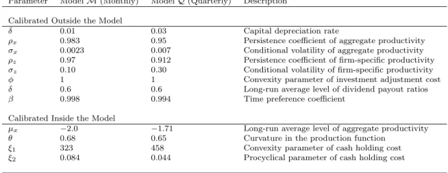
We calibrate 12 parameters δ, ρ¯ x,σx,ρz, σz, φ, δ, β, µx, θ, ξ1, ξ2
both in monthly and quarterly frequencies to facilitate the comparison of our results with those from the empirical literature. The monthly model is denoted as Model M, and the quarterly model, as Model Q. The first parameter set ¯δ, ρx,σx,ρz, σz, φ, δ, β is calibrated out-side the models, and the second parameter set (µx, θ, ξ1, ξ2) is calibrated inside the models following the idea of generalized method of moments. Table I reports the parameter values that we use to solve and simulate the models.
(Abel and Eberly (2002)). The persistence of the aggregate productivity process (ρx)
is 0.95 and its conditional volatility (σx) is 0.007, which are quarterly values. 0.983
and 0.0023 are the monthly values of those parameters,ρx andσx,respectively. These values are consistent with Cooley and Prescott (1995). For the persistence (ρz) and
conditional volatility (σz) of the firm-specific productivity shock, we set ρz = 0.97
and σz = 0.10 for monthly frequency. These values are chosen from the related
literature (e.g., Zhang (2005), Li, Livdan, and Zhang (2009), and Livdan, Sapriza, and Zhang (2009)) to generate a plausible amount of dispersion in the cross-sectional distribution of firms. We setρz = 0.912 and σz = 0.30 for quarterly frequency. The
average payout ratio (δ) is calibrated to be 60%, borrowed from the average value of aggregate payout ratios from 1981 to 2007 in CRSP/COMPUSTAT merged data. We choose the time preference parameter, β = 0.998 on monthly and β = 0.994 on quarterly.
Regarding the second set of parameters (µx, θ, ξ1, ξ2), we calibrate those param-eters using the following procedure.12
1. Set initial values for group Λ0 = (µ0
x, θ0, ξ01, ξ20). 2. Solve the value function V (Sit) such that,
(a) Each grid on the compact set S represents each firm in the market. (b) By backward induction, solve the V0(S
it) and V1(Sit) on each iteration,
and pick the bigger value.
3. From the converged value function V (Sit), we have the operating profit
func-tion (profitability) and endogenous policy funcfunc-tions (investment-capital ratio, 12The convexity parameter of investment adjustment cost (φ) is normalized to one to conserve the number of parameters used in our numerical study.
disinvestment-capital ratio, and dividend policy) such that, Zit = Π (Sit) Kit ,I+(Sit) Kit ,I−(Sit) Kit , ait; Λ 0 ,
in which, I+ is the net investment and I− is the net disinvestment.
4. Define the generalized moments of policy functions as, 1 n n X i=1 Zit−E[Zit] = ¯Z(Λ)−Z,
in which n is nK ×nx×nz, (nK: number of grids on SK, nx: number of states of x, and nz: number of states ofz).
5. By iterating the process from step 1 to step 4, we solve the minimization problem for the parameters as follows,
ˆ
Λ = arg min Λ
¯
Z(Λ)−Z0W Z¯(Λ)−Z,
in which W is a weight matrix, and we use identity matrix in this study. Our method is not the same as the conventional simulated method of moments since we do not generate random numbers to compute the moments of endogenous policy functions. Rather, generated moments are the average numbers of target val-ues from points on all grids of the compact state space while iterating value functions regarding the values of Z. The average monthly profitability defined as the oper-ating profit to the capital ratio (Π/K) is 1.25%, the value of the average monthly net investment ratio (I+/K) is 1.25%, for the net disinvestment (I−/K), 0.17% is
the average value on monthly frequency. These values are reported by Abel and Eberly (2002). The average proportion of firms in CRSP that paid dividends in a period from 1926 to 1999 is 49%. This number is borrowed from Fama and French (2001). The calibrated parameters are Λ = (−2.0,0.68,323,0.084) for ModelMand
(−1.71,0.65,458,0.044) for Model ModelQ. The curvature parameter in the produc-tion funcproduc-tion (θ) is monthly 0.68 and quarterly 0.65, close to the values suggested by Livdan, Sapriza, and Zhang (2009) or the average values estimated by Cooper and Ejarque (2001), Cooper and Ejarque (2003), Hennessy and Whited (2005), and Hennessy and Whited (2007). The long-run average level of aggregate productivity (µx) is −2.0 for Model M and −1.71 for Model Q, which are higher than other free
cash flow asset pricing models (e.g., Zhang (2005), Li, Livdan, and Zhang (2009), and Livdan, Sapriza, and Zhang (2009)). The difference may come from the way this parameter is retrieved. They calibrateµx and time-varying γ exogenously by fitting
the first and second moments of risk-free rate data. Meanwhile, we use only firm characteristics data to calibrate it. Convexity parameter of the cash holding cost (ξ1) and procyclical parameter of cash holding cost (ξ2) are 323, 458, and 0.084,0.044 on monthly and quarterly frequencies, respectively.
2. Investment, Dividend Policy, and Cash Holdings
Panel (A)’s in Figures 5-8 display optimal investment behaviors as a function of capital and productivity shocks (K,x,z). First, we observe that optimal investments increase until capital stock (K) reaches level at which dividend payouts begin. When this occurs, investment drops off by about the half of where it used to be. As discussed,
x and z determine the amount of investments, and they have positive relationships with investment.
Panel (B)’s in Figures 5-8 show that the investment-capital ratios (I/K) given
xandz decrease as capital stock increases, because of diminishing returns to scale of capital. This is consistent with the view that young firms are more likely to invest their resources in capital compared to mature firms. What is new in our model is that a firm will execute a one-time discrete reduction of investment in its life cycle, as it
grows. The discrete shift in investment results from the lumpy behavior of dividend policy, as we discussed earlier, because dividend payment substitutes for the amount of investment. However, we want to emphasize that this does not necessarily imply that investment and dividend payout will feature negative correlation, since adjustment is costly for both investment and dividend and therefore, frequent changes of these variables are unlikely to prevail. Only a few observations show conditionally negative correlations, and the unconditional correlation between investment and dividend does not need to be negative, because it can depend more on firm profitability, level of capital, and related, firm age.
Firms with the smaller amount of capital invest more, and the investment de-creases rather abruptly as capital is accumulated. Panel (C)’s in Figures 5-8 show the optimal dividend policies. Zero dividend equity ratios mean that firms are not paying dividends, and positive numbers show that the firms pay dividends. Firms with higher x and z are more likely to initiate their dividend payouts earlier, since those firms will accumulate capital faster, hence they tend to mature earlier than other firms. Recall that our model has the cash holding cost motivated in part by the agency cost resulting from the tension between equity holders and the firm man-ager. Thus, accumulated capital will lead to larger operating incomes which trigger dividend payout.
It is natural to think that the propensity to pay dividends (PPD), P{a= 1|S}
and firm-characteristics such as profitability, investment, and the market value of capital are associated with each other. Figures 5-8 suggest that our model indeed replicates the stylized facts in Fama and French (2001) as mentioned earlier: Asset prices generated by the model are consistent with the firm characteristics.
Panel (D)’s in Figures 5-8 plot the value functions of firm dynamics (2.2) which are the present values of cash flows into cash holdings. These figures show that asK,
x,and z increase, a young firm’s present value of cash flows increases, but the value of a mature firm which pays dividends decreases. For a young firm, the increases in
x and z make its managerial cost increase due to the procyclical cash holding cost, and force the young firm to invest more cash in capital. Then, this procyclical effect expedites the young firm’s initiation of dividend payouts earlier than when it has lower
xandz. For a mature firm, although it also shares this procyclicality channel, it will face a relatively limited investment opportunity set due to its large capital. Thus, the mature firms are bound to solve a more constrained optimization to minimize the total managerial cost. This renders the mature firms to incur higher cash holding cost than when it was young. This also makes them to pay more dividends to reduce the cash holding cost. Thus, the present values of cash flows for the mature firms will become smaller than those of younger firms, and decrease inxand z, ceteris paribus.
3. Analyzing Stock Returns
Now, to analyze the expected market return and cross sections of expected stock returns, we simulate 200 artificial panels, each of which has 2703 firms on each state
x. Model M simulates average 2100 months to generate one panel, and Model Q simulates average 1200 quarters on each panel. The cash flows are discounted by the computed pricing kernels and summed up to Pitj in each panel j, where j = 1, ...200, until all Pitj’s converge, following the pricing formula (2.6). Then, the final stock price of firm i at time t, Pit, is computed by the average value of {Pitj}200j=1 . Finally, the expected stock returns are computed using Markov transition matrices of x and z approximated by the method in Adda and Cooper (2003). We calculate the expected value-weighted stock returns on each state,x, and consider them as the market portfolio returns, or the wealth portfolio returns. In addition, the risk-free rate is computed by the reciprocal of the average value of Mt,t+1 using the simulated
data.
a. Aggregate Market Values
Table II reports the unconditional moments of market variables such as equity pre-mium, risk-free rate, price-dividend ratio, book-to-market equity ratio, aggregate dividend growth, and the volatilities of those variables as well. The U.S. historical data are collected from various sources. The average equity premium ranges from 4% to 8% according to the related literature. The volatility of market return is 19.4%,
according to Guvenen (2009), computed using Standard and Poor’s 500 index during the period of 1890-1991. The empirical Sharpe ratio is 0.50, which is from Cochrane (2005). The fitted model generates reasonable values for the expected equity pre-miums compared to the data. Model M with γ = 3 and Model Q with γ = 3.5 have the volatilities of stock market returns of 20.1% and 20.9%, which is close to 19.4%. The cross-sectional volatility of individual stock returns is from 25% to 32% reported by Zhang (2005). Model Mreports higher volatilities than this, but Model Qreports somewhat lower values. The actual rates of capital gain and dividend price ratio are 2.1% and 4.70% from Fama and French (2002) covering from 1872 to 2000. This means that the dividend price ratio is about 123% larger than the capital gain in constituting the market equity return. The dividend price to capital gain ratios (Dt+1/∆Pt+1) from all models are around 2.5, which is close to the empirical value. Turning to the risk-free rate, annualized U.S. risk-free rate is 1.8% with volatility of 3.0% according to Zhang (2005). The corresponding risk-free rates in Model M are relatively higher than data. The historical standard deviation of risk-free rate is more volatile compared to the simulated values in Model M. Model Q creates more volatile risk-free rates than ModelM. However, there are several other studies reporting that the risk-free rate has much lower volatility, and therefore, we believe
that our result on the risk-free rate is reasonable.
Regarding the Sharpe ratio, the simulated Sharpe ratios have a wide range from 0.23 to 0.59 in Model M, and the range from 0.27 to 0.54 in Model Q. When relative risk aversion is between 3 and 4, our results are consistent with the empirical counterpart. ModelMgenerates aggregate dividend growths around 2.40%, with the aggregate dividend growth volatilities at about 11.4%. ModelQgenerates somewhat higher aggregate dividend growth volatilities of around 13%, which is close to the data, 13.4%, reported by Guvenen (2009), and the aggregate dividend growths are around 2.56%,which is fairly close to the empirical value, 2.5%. The average book-to-market equity ratio (BE/M E) is 0.67 and its standard deviation is 0.23 according to Zhang (2005). ModelQrepresents values of 0.62 and 0.24 respectively, which are again fairly close to the data. We also compute (BE/M E)payer/(BE/M E)non-payer which is the ratio of average book-to-market equity ratios of dividend payers and non-payers. The empirical value is 1.32,computed using the CRSP/COMPUSTAT merged data. This value states that high book-to-market firms are more likely to pay dividends (Smith and Watts (1992) and Baker and Wurgler (2004b)), and it is consistent with our theory for the value premium. All of our simulated values are greater than 1, and ModelQhas values close to the data. For the average price-dividend ratio, as relative risk aversion increases, models yield lower rates of price dividend ratios, but higher volatilities of them. Results suggest that our model explains the data reasonably well with relative risk aversion around 3.
Thus, the model replicates the moments of key financial market variables in both monthly and quarterly versions. Note that all the parameters are fitted by matching the moments of variables related to firm characteristics, not financial variables. The model can capture the level and volatility of the historic equity premium, while keep-ing plausible values for the first two moments of the risk-free rates. However, we must

![Table IV. Logit Regressions of Propensities of Payouts: Dividend Payment and Stock Repurchase, 1962 to 2009 Π it A it I itA it M itAit P M E it P ayer it 7.55 -3.44 -0.63 1.64 [14.5] [-5.5] [-11.9] [12.4] T otalpay it 6.65 -3.16 -0.58 1.54 [14.3] [-5.44] [](https://thumb-us.123doks.com/thumbv2/123dok_us/1771605.2751941/88.918.329.618.458.635/table-regressions-propensities-payouts-dividend-payment-repurchase-otalpay.webp)


![Table VII. Continued ˆ a P t ˆ a N Pt T P t P −N P ˆ a Rt ˆ a N Rt SR R−N Rt r V t+1 − r t+1G -0.19 -0.18 0.09 -0.21 -0.26 -0.02 [0.20] [0.20] [0.54] [0.19] [0.11] [0.89] r S t+1 − r t+1B 0.19 0.44 -0.43 0.17 0.28 -0.14 [0.20] [0.00] [0.00] [0.31] [0.08] [](https://thumb-us.123doks.com/thumbv2/123dok_us/1771605.2751941/92.918.263.686.410.811/table-vii-continued-pt-rt-rt-sr-rt.webp)