University of Pennsylvania
ScholarlyCommons
Marketing Papers
Wharton Faculty Research
1-2014
Understanding the Effect of Advertising on Stock
Returns and Firm Value: Theory and Evidence
From a Structural Model
Maria Ana Vitorino
University of Pennsylvania
Follow this and additional works at:
http://repository.upenn.edu/marketing_papers
Part of the
Marketing Commons
This paper is posted at ScholarlyCommons.http://repository.upenn.edu/marketing_papers/203 For more information, please [email protected].
Recommended Citation
Vitorino, M. A. (2014). Understanding the Effect of Advertising on Stock Returns and Firm Value: Theory and Evidence From a Structural Model.Management Science, 60(1), 227-245.http://dx.doi.org/10.1287/mnsc.2013.1748
Understanding the Effect of Advertising on Stock Returns and Firm Value:
Theory and Evidence From a Structural Model
Abstract
This paper brings structural modeling to the literature on financial research in marketing. I propose a dynamic investment-based model to understand the impact of advertising expenditures on stock returns and firm value. In addition, by interpreting advertising expenditures as an investment in brand capital, the approach in this paper provides a novel way to measure brand equity grounded in economic theory. Using the Euler equations from the firm’s maximization problem, I derive closed-form expressions for the firm’s equilibrium stock returns and market value, which depend on observable firm characteristics. I test the model’s predictions by the generalized method of moments and data from a large cross section of publicly traded firms. The model is able to match simultaneously the pattern of average stock returns and firm values of portfolios sorted on advertising expenditures that standard asset pricing models cannot. The estimation results also show that brand equity accounts for a substantial fraction of firm market value (about 23%), and that this value varies substantially across industries. Implications of the findings for research at the intersection of marketing and finance are discussed.
Keywords
advertising, brand value, stock returns, structural model, marketing and finance
Disciplines
Understanding the Effect of Advertising on Stock
Returns and Firm Value: Theory and Evidence from
a Structural Model
∗Maria Ana Vitorino† Carlson School of Management
University of Minnesota January 2013
Abstract
This paper brings structural modeling to the literature on financial research in
mar-keting. I propose a dynamic investment-based model to understand the impact of
advertising expenditures on stock returns and firm value. In addition, by interpreting advertising expenditures as an investment in brand capital, the approach in this paper provides a novel way to measure brand equity grounded in economic theory. Using the Euler equations from the firm’s maximization problem I derive closed-form expressions for the firm’s equilibrium stock returns and market value, which depend on observable firm characteristics. I test the model’s predictions by the Generalized Method of Mo-ments and data from a large cross-section of publicly traded firms. The model is able to match simultaneously the pattern of average stock returns and firm values of portfolios sorted on advertising expenditures which standard asset pricing models cannot. The es-timation results also show that brand equity accounts for a substantial fraction of firm market value (about 23%), and that this value varies substantially across industries. Implications of the findings for research at the intersection of marketing and finance are discussed.
Keywords: Advertising, Brand Value, Stock Returns, Structural Model, Marketing and Finance.
JEL Classification: D92, E22, G12, G14, G32, M31, M37
∗
I am especially indebted to Frederico Belo for many helpful discussions and detailed comments. I would like to thank Franklin Allen, Dominique Hanssens, Zvi Eckstein, Alex Edmans, Jonathan Knowles, Xueming Luo, Lopo Rego and David Reibstein, Wei Xiong (the editor), and one anonymous area editor and two anonymous referees for their thoughtful suggestions and comments. I also thank seminar participants at the University of Pennsylvania (Wharton – Finance Department), participants at the 2010 Marketing Science conference, and participants at the Marketing Strategy Meets Wall Street II conference for comments. I gratefully acknowledge the financial support from the Rodney L. White Center for Financial Research at the University of Pennsylvania. All errors are my own.
†
1
Introduction
Understanding the effect of advertising (and other marketing variables) on firm performance is an important question for managers, investors and researchers. Recognizing the impor-tance of this question, a literature at the intersection of marketing and finance has emerged. This literature documents strong correlations between firm advertising expenditures, firm value and stock returns.1 The strength of these correlations is an interesting and important finding on its own. However, endogeneity problems make these relationships difficult to interpret in the absence of theoretical models that explicitly link advertising expenditures with both firm value and stock returns (and risk).
In this paper, I propose a dynamic structural investment-based model to understand and quantitatively evaluate the impact of advertising expenditures on firm value, stock returns and risk in a setup in which these variables are jointly determined. I interpret firm advertising expenditures as an investment to create brand capital, an intangible asset that summarizes consumers’ awareness of the goods and services produced by the firm. This brand capital stock may help firms increase sales through, for example, increased customer loyalty, visibility, or perceived quality. Thus, brand capital stock is potentially an important component of firm market value. In addition, as an investment in capital stock, optimal advertising expenditures are related to a firm’s cost of capital (risk), and thus advertising expenditures are potentially informative about a firm’s expected stock returns.
The approach used in this paper brings structural modeling to the literature on financial research in marketing. Structural approaches have been used in the marketing literature with most applications in areas related to industrial organization economics.2 To the best
of my knowledge, the link between advertising and firm value has been studied separately from the relationship between advertising and risk and only through the use of reduced form approaches. Such studies, while able to show the patterns in the data, cannot use the data to test theories regarding what drives the observed empirical links. The model I propose here
1
I review the empirical findings in Section 2 below.
2
For an excellent review and discussion of the advantages and disadvantages of structural work in mar-keting see Chintagunta et al. 2006.
can be used to understand the observed correlations in the data. In addition, the estimation of the model provides a new economics-based paradigm for measuring brand equity, thus contributing to the marketing literature on brand valuation.
I consider the neoclassical model of investment as the starting point for my analysis, fol-lowing Belo, Lin, and Vitorino (2013).3 The model is augmented with brand capital, which is introduced as an additional input in the firm’s production technology. The model features a cross-section of firms. Firm managers make physical capital investment and advertising decisions to maximize the market value of the firm. As standard in the neoclassical theory of investment, the only frictions in the model are the existence of adjustment costs in the two capital inputs, and the importance of these costs is estimated in the data. In particular, building brand capital can be costly because, in addition to the direct advertising expen-diture costs, planning and executing advertising activities (even if outsourced) take away resources (e.g. workers) from other productive activities and are typically associated with promotional activities.
Building on Liu, Whited, and Zhang (2009), and using the Euler equations from the firm’s maximization problem, the model expresses the firm’s equilibrium stock returns and market value as a function of firm characteristics (e.g. advertising expenditures, physical capital investment and sales). These functional forms depend on the parameters of the firm’s technology. For stock returns, the model predicts that firms with high marginal product of physical and brand capital, high growth rates of physical capital and advertising investment rates, and high market leverage ratios have higher average stock returns. For firm value, the model predicts that firms with high physical capital and advertising investment rates, as well as high brand capital to physical capital ratios have higher average scaled market values (Tobin’s Q).
I test the model’s predictions using the Generalized Method of Moments (GMM) on
3
The neoclassical model of investment provides a natural starting point for my analysis since this ap-proach has been successfully used to understand several asset pricing facts. Important applications of the neoclassical theory of investment to asset pricing include Cochrane (1991), Zhang (2005) , Liu, Whited, and Zhang (2009) and Li, Livdan, and Zhang (2009). Additional studies incorporating intangible capital into this framework include Hansen, Heaton, and Li (2005), Li and Liu (2010), Gourio and Rudanko (2010) and Belo, Lin, and Vitorino (2013).
data from a large cross-section of publicly traded firms. As moment conditions, I use the model’s implied stock returns and market value to investigate if these values are, on average, equal to the corresponding averages observed in the data. To construct the model’s implied stock returns and market values, I need data on several firm characteristics, including the intangible (and hence unobserved) brand capital stock of each firm. Following Belo, Lin, and Vitorino (2013), I construct a firm-level brand capital stock measure from advertising expenditures accounting data using the perpetual inventory method. Finally, the GMM estimation of the model is performed on portfolios sorted on advertising growth because one of the goals of this paper is to understand the link between advertising expenditures with both firm value and stock returns, previously documented in the literature.
The empirical results can be summarized as follows. The investment-based model with brand capital captures well both the cross-sectional variation in average stock returns across the advertising growth portfolios, as well as the observed cross-sectional variation in firm values with reasonable parameter values for the firm’s technology. The model generates very low pricing errors and is not rejected in the data by theχ2Hansen (1982) test. Importantly, the investment-based model with brand capital significantly outperforms standard asset pricing models such as the CAPM, the Fama and French (1993) three-factor model, and the Carhart (1997) four-factor model in matching the average returns of the advertising-growth portfolios. When the model is used to match average returns, the mean absolute pricing error generated by the model is only0.21%per annum. This average pricing error is considerably smaller than the pricing error of the CAPM (4.94%per annum), of the Fama-French model (3.16%), and of the Carhart model (5.49%).
The parameter estimates show that the value of brand capital (brand equity) accounts for a substantial fraction of firm market value. The value of firms’ brand capital stock is estimated to represent on average about23%of firms’ total market value. In addition, this value ranges from close to zero for commodities (e.g. Steel, Oil) to about 30−60% for consumer goods. The importance of brand capital in firm value across industries seems to vary in a predictable way, thus suggesting the measure of brand capital used here has
reasonable properties. The importance of brand capital tends to be stronger in industries with more consumer product orientation than in industries with low consumer product orientation. The findings highlight the importance of brand capital in firm valuation.
The empirical findings also show the relevance of brand capital adjustment costs for understanding brand value. In addition to the explicit cost of advertising, augmenting the brand capital stock (i.e. creating a brand name) is estimated to be costly: the estimated parameter values imply that brand capital adjustment costs represent, on average, around
8%of firms’ annual sales. Because firms need to spend substantial resources to increase the brand capital stock, this helps to explain why brand names (i.e. installed brand capital) are an important component of firm market value.
The good empirical fit of the investment-based model with rational and profit maximizing firms suggests that the correlations between advertising expenditures, firm value and stock returns documented by previous literature are consistent with a risk-based interpretation. Advertising is a form of investment which creates brand capital. As a form of investment, standard reasoning from the Q-theory of investment suggests that advertising expenditures are determined by the firm’s cost of capital (expected stock returns), which is determined by the firm’s risk. Therefore, firms with high advertising growth invest more in brand capital and have lower cost of capital, implying lower expected returns going forward, than firms with low advertising growth.
The model and estimation results also have practical implications. The model provides a simple straightforward formula to compute the firm-level value of brand capital (brand equity). To compute this value, only two inputs are required: readily available (current and past) firm-level advertising expenditure data and the parameter estimates of brand capital adjustment costs obtained here. The new measure complements other research techniques and approaches that have been proposed in the brand valuation literature, thus helping researchers and practitioners better capture the complexity of brand equity.
The paper proceeds as follows. Section 2 discusses the related literature and highlights the contribution of the paper to the literature at the intersection of marketing and finance.
Section 3 describes the dynamic investment-based model with brand capital, derives the testable implications for the cross-section of stock returns and firm values, and discusses the predicted links between firm characteristics and stock returns and market value in the model. Section 4 presents the estimation methodology, the data used, and a summary of the facts linking advertising expenditures to stock returns and firm value in the data. Section 5 presents the empirical results and contrasts the fit of the investment-based model with that from standard asset pricing models. Section 6 presents the value of brand equity at the industry-level as well as at the firm-level, implied by the estimation of the model. Finally, Section 7 discusses the implications of the findings for research at the intersection of marketing and finance.
2
Related Literature
The work in this paper is related to several strands of literature at the intersection of marketing and finance.
First, this paper contributes to research at the intersection of marketing and finance which studies the effect of advertising (and other marketing variables) on firm performance.4 As I discuss in Section 4.4, this literature documents correlations between advertising expen-ditures, firm value, and stock returns. The findings in this literature include the observations that: (i) firms’ current advertising expenditures are positively contemporaneously correlated with firms’ market value and stock returns and (ii) firms’ current advertising expenditures and future stock returns are negatively correlated. This empirical evidence is difficult to in-terpret due to endogeneity problems in these correlations. By explicitly linking advertising expenditures with firm value and stock returns (and risk), the structural model proposed here provides an economic framework for interpreting the empirical evidence.
In addition to the previous findings, this strand of the literature also finds that, either
4
Srivastava, Reibstein, and Joshi (2006), Srinivasan and Hanssens (2008), Conchar, Crask, and Zinkhan (2005) and Mizik and Jacobson (2009) provide excellent reviews of the literature in marketing studying the link between marketing activities (including advertising expenditures), firm value and stock returns. Recent applications include Rego, Billett, and Morgan (2009) and Joshi and Hanssens (2010). Schmalensee (1972) and Bagwell (2007) survey the literature on the economic analysis of advertising.
through event studies or by testing standard asset pricing models such as the capital asset pricing model (CAPM) or the Fama-French (1993) three-factor model, there are statistically significant abnormal returns associated with advertising expenditures (I confirm this finding in Section 5.1.2). This fact is typically interpreted as evidence against the efficient market hypothesis (EMH), and several behavioral explanations for the findings have been proposed. For example, Lou (2010) interprets the positive abnormal returns associated with adver-tising expenditures as consistent with the hypothesis that firm managers use adveradver-tising expenditures to attract investors’ attention and, thus, maximize short-term stock market prices to their (or existing shareholders) benefit. Other explanations, summarized in Joshi and Hanssens 2010, include spillover and signaling effects.5
An alternative explanation, however, for why the standard asset pricing models generate abnormal returns is that these models are misspecified in the sense that they may not be capturing all sources of systematic risk. In particular, these models may not capture the systematic risk associated with intangible assets such as brand equity. The model proposed here allows me to formally investigate this hypothesis in the data. By linking the firm’s equilibrium stock returns and firm value directly to firm characteristics, I can test the predictions of the model without having to explicitly specify the sources of systematic risk in the economy. That is, in this investment-based approach, firm characteristics are sufficient statistics to characterize firm risk. In turn, this helps making this approach robust to misspecifications of the sources of systematic risk in the economy.6
This paper also relates to the literature on brand valuation because it develops a new methodology to estimate brand value (typically referred to as brand equity) which is based on readily available accounting and asset price data. This methodology complements ex-isting measures and encompasses many of (if not all) the characteristics listed by Ailawadi, Lehmann, and Neslin (2003) as being important for any measure of brand equity.
5
The spillover effect indicates that advertising increases the stock market’s familiarity with the firm, thereby increasing stock ownership, liquidity, and firm value (Frieder and Subrahmanyam 2005; Huberman 2001; Joshi and Hanssens 2010). The signaling effect indicates that advertising spending can be a signal of financial well-being or competitive viability (e.g., Joshi and Hanssens 2010).
6
See Lin and Zhang (2011) for a detailed discussion of the advantages of using firm characteristics in empirical research on asset pricing.
The importance of brand value to understand firm value is well established in the mar-keting literature. The intangible nature of a brand represents a challenge in this literature because of the need to translate a firm’s brand value/equity into a quantitative measure.
Since Aaker (1991), several researchers and practitioners have proposed alternative meth-ods for assessing the value of a brand. Generally, it is agreed that no single measure tells a complete story. Existing measures of brand equity typically fall into one of three cate-gories.7,8 First, customer mindset-related measures are based on consumer surveys seeking to assess customers’ awareness, attitudes, associations, attachments, and loyalties towards a brand. Much of the academic research (e.g. Aaker 1996, Keller 2003) and work by consult-ing firms (e.g., Millward Brown’s BrandZ and Young and Rubicam’s BrandAsset Valuator) has focused on this type of metrics. The second category of measurement focuses on the measures related to product-market outcomes. The most commonly measured unit is the price premium that the brand commands over a base product (e.g. Park and Srinivasan 1994, Sethuraman 1996, Goldfarb, Lu, and Moorthy 20099). Other measures of this type include the constant term in sales response models (e.g. Srinivasan 1979 and Kamakura and Russell 1993). Measures in this category rely on data collected through surveys or on actual purchase data (usually for a single product category). The final category of measurement is based on financial market performance. Specifically, these assess the value of a brand in terms of financial assets. Purchase price, when a brand is sold or acquired (Mahajan, Rao, and Srivastava 1994), and discounted cash flow dimensions of licensing fees and royalties are measurements of this type.
Simon and Sullivan (1993) were the first to propose a technique for estimating a firm’s brand equity based on the financial market value of a firm. The model proposed in this paper is in the spirit of Simon and Sullivan’s in the sense that it also constitutes a financial
7
Some metrics, such as the Interbrand measure, are an hybrid of different approaches.
8
For a more detailed description of these categories, including the advantages and disadvantages of each approach see Ailawadi, Lehmann, and Neslin (2003), Keller and Lehmann (2006)) and Srinivasan, Hsu, and Fournier (2011).
9It should be noted that Goldfarb, Lu, and Moorthy (2009) distinguishes itself from the other papers
here listed due to the fact that it uses an equilibrium methodology that produces brand value estimates in profit terms. The authors illustrate their proposed method using market-share data on the ready-to-eat breakfast cereals product category.
market-based approach to brand valuation. The key distinction between my work and theirs is that I examine the links in the data using a structural model whereas Simon and Sullivan’s analysis is based on a reduced-form approach, which limits the economic interpretation of their findings. In addition, I provide a comprehensive empirical analysis by combining both time series and cross sectional data, whereas Simon and Sullivan focus on cross-sectional data in a single year.
By modeling firms’ optimal investment and advertising behavior, the structural investment-based model proposed here provides an alternative, yet complementary, economics-investment-based paradigm to link equity valuation to brand capital and other accounting information. This methodology takes into account that both advertising expenditures and firm value are jointly determined in equilibrium, thus accounting for endogeneity problems that affect reduced-form approaches.10 In addition, the estimates in the investment-based model can be directly
linked to deep structural parameters, in particular, to the characteristics of the firm’s pro-duction technology. This is useful because it allows me to investigate if the model fits the data with reasonable parameter values, an important criteria in the evaluation of any model. Finally, the focus on brand capital is closely related to the asset pricing literature on intangible capital and firm risk in particular to the work by Belo, Lin, and Vitorino (2013) and by Li and Liu (2010).11 The theoretical investment-based model used here is based on Belo, Lin, and Vitorino (2013). The key distinction between my analysis and theirs is that I evaluate the model mechanism by estimating the model using real data, whereas
10
The endogeneity (or joint determination) that exists between advertising and stock returns is a well recognized issue in the marketing-finance literature which few researchers have tried to address. For example, Joshi and Hanssens (2010) have used VAR models to mitigate the endogeneity concerns. But, as recognized in the literature (see Srinivasan and Hanssens 2008), persistence models (of which VAR models are part of) are inherently reduced-form models thus failing to provide a rational interpretation for the obtained effects.
11Related papers include: Gourio and Rudanko (2010) who study the implications of customer capital
for firm level and aggregate dynamics; Hansen, Heaton, and Li (2005) who study the risk characteristics of intangible capital; Hsu (2009) who shows that technological innovations forecast stock excess returns at the aggregate level using R&D data, a form of investment in intangible capital; Chan, Lakonishok, and Sougiannis (2001) who document a positive relation between R&D intensity and firms’ future stock returns and Li (2011) who shows that this positive relation is only present in R&D intensive firms; Lin (2011) who explains the link between R&D expenditures and asset prices in a theoretical model; and Eisfeldt and Papanikolaou (2013) who study the link between organizational capital and firm risk. My work differs for these papers because I focus on a distinctive measure of intangible capital, brand capital, and I perform a structural estimation of the model in the data.
they evaluate the model by calibration and simulation. The estimation approach allows me to talk about model errors in real data, and thus quantitatively evaluate how well the model fits the empirical facts. Also, in contrast to Belo, Lin, and Vitorino (2013), I do not study the relationship between advertising expenditures and the firm’s external financing policies. Similar to the approach in this paper, Li and Liu (2010) quantify the importance of R&D capital (a form of intangible capital) for understanding stock returns in a neoclassical investment-based model and using structural estimation. The key difference between my work and Li and Liu (2010) is that I focus on a different measure of intangible capital (brand capital) thus relating the analysis to the marketing literature. In addition, I investigate the ability of the model to explain the cross-section of firms’ scaled market values (Tobin’s Q) jointly with stock returns. My findings complement those in Li and Liu (2010) by showing the importance of alternative measures of intangible capital for understanding firm risk, as well as by confirming the large economic magnitude of intangible capital adjustment costs first documented in Li and Liu (2010).
3
A Structural Investment-Based Model of Advertising
I propose a dynamic investment-based model to study the link between advertising, firm value, and stock returns, and to estimate the value of brand capital in the data. The model builds on the neoclassical investment-based model in Liu, Whited, and Zhang (2009), and is augmented with brand capital, following the approach in Belo, Lin, and Vitorino (2013). In the model, brand capital is a productive input because it helps firms increase sales through, for example, increased customer loyalty, visibility, or perceived quality.12 Firms accumulate brand capital through advertising expenditures, and make optimal production decisions to maximize firm value. Optimal investment and advertising establish an endoge-nous link between advertising expenditures and firm stock returns and market value.
I first describe the firm’s value-maximization problem and then derive testable
implica-12
See, for example, Aaker (1991), Simon and Sullivan (1993) and Bagwell (2007) for a detailed discussion of alternative economic explanations for why and how consumers respond to advertising.
tions for the cross-section of stock returns and firm value.
3.1 Technology
Time is discrete and the horizon infinite. Firmi uses capital,Kit, brand capital, Bit, and
a vector of costlessly adjustable inputs to produce an homogeneous output. The operating profit functionY is an increasing function of the inputs,Yit≡Y(Kit, Bit, Xit),in whichXit
is a vector of exogenous aggregate and firm-specific productivity shocks (higher values of
Xit increase profits). Yit displays constant returns to scale such that Yit =Kit∂Yit/∂Kit+
Bit∂Yit/∂Bit, in which ∂ denotes partial derivative. The marginal operating profits from
physical capital and brand capital are parameterized as (see also Love 2003):
∂Y(Kit, Bit, Xit) ∂Kit = αK Yit Kit , (1) ∂Y(Kit, Bit, Xit) ∂BKit = αB Yit Bit . (2)
in whichYit is measured as sales, αK >0 is physical capital’s share, and αB >0 is brand
capital share.
Physical capital stock evolves as:
Kit+1=Iit+ (1−δitK)Kit, (3)
in whichIit is capital investment andδKit is the depreciation rate of capital. Similarly, the
brand capital stock evolves as:
Bit+1=Ait+ (1−δB)Bit, (4)
in whichAitare the firm’s advertising expenditures andδB is the depreciation rate of brand
capital.
Firms incur adjustment costs when investing. The adjustment cost function, denoted
linearly homogeneous inIit, Kit, Ait, andBit. I consider a simple quadratic adjustment-cost function: Φt≡Φ(Iit, Kit, Ait, Bit) = 1 2 ηK Iit Kit 2 Kit+ 1 2 ηB Ait Bit 2 Bit, (5)
in which ηK > 0 and ηB > 0 are the adjustment cost parameters for physical capital and
brand capital, respectively.
In this specification, as standard in the neoclassical theory of investment, the capital adjustment costs include planning and installation, learning the use of new equipment, or the fact that production is temporarily interrupted. Similarly to physical capital, in this specification, firms also incur adjustment costs when expanding the stock of brand capital.13 These costs capture the notion that planning of advertising campaigns is costly and takes away resources (e.g., workers) from other productive activities. In addition, advertising expenditures may be associated with an increase in customer support, promotional activities, etc. Further, small scale local advertising campaigns usually done in-house are less expensive than large scale national campaigns often done by professional advertising agencies. As such, adjustment costs are likely to increase with advertising expenditures.
3.2 Taxable Profits and Firm Payout
Following Hennessy and Whited (2007), at the beginning of time t, firm i can issue one-period debt, denoted bit+1, which must be repaid at the beginning of t+ 1. The gross
corporate bond return on bit, denoted Rbit, can vary across firms and over time. Taxable
corporate profits equal operating profits less advertising expenditures, capital depreciation, adjustment costs, and interest expenses:
Y(Kit, Bit, Xit)−Ait−δitKKit−Φt−(Rbit−1)bit.
Here, adjustment costs are expensed, consistent with treating them as foregone operating
13
See Gourio and Rudanko (2010) for a similar assumption in the context of customer capital, which is similar in spirit to brand capital (i.e. both stock variables capture customer loyalty).
profits.
Letτt denote the corporate tax rate at timet. The payout of firm iis then given by:
Dit≡(1−τt)[Y(Kit, Bit, Xit)−Ait−δitKKit−Φt]−Iit+bit+1−Rbitbit+δKitKitτt+τt(Ritb−1)bit,
in whichδK
itKitτt is the depreciation tax shield and τt(Rbit−1)bit is the interest tax shield.
3.3 The Firm’s Maximization Problem
LetMt+1be the stochastic discount factor fromttot+1, which is correlated with the
aggre-gate component of the productivity shockXit. The firm makes physical capital investment,
advertising and debt decisions to maximize the cum-dividend market value of equity. The maximization problem can be formulated as follows:
Vit≡ max {Iit+s,Kit+s+1,Ait+s,Bit+s+1,bit+s+1}∞s=0 Et "∞ X s=0 Mt+sDit+s # , (6)
subject to the physical capital and brand capital accumulation equations (3) and (4) and to a transversality condition that prevents firms from borrowing an infinite amount of debt:
limT→∞Et[Mt+T bit+T+1] = 0.
3.4 Equilibrium Stock Returns and Firm Value
Proposition 1 states the key results from the theoretical model. This proposition expresses the firm’s equilibrium market value and stock returns as a function of the firm’s observable characteristics.
Proposition 1 (Firm Value and Stock Returns) Define Pit ≡ Vit −Dit as the
ex-dividend market value of equity. Also, let KQit and BQit be the present value multipliers
associated with equations (3) and (4). KQit andBQit are the marginal benefits of an
implies that
Pit+bit+1 = KQitKit+1
| {z }
Value of Physical Capital
+ BQitBit+1
| {z }
Value of Brand Capital
, (7) in whichKQit ≡1 + (1−τt)η2K Iit Kit and BQit ≡(1−τt) 1 +ηB2 Ait Bit .
In addition, the firm’s value-maximization implies that Et[Mt+1RitI+1] = 1, in which
RIit+1 is the physical capital investment return, defined as:
RIit+1≡ (1−τt+1) αKKYitit+1+1 +12 ηKKIitt+1+1 2 +δitK+1τt+1+ (1−δKit+1) 1 + (1−τt+1)ηK2 Iit+1 Kit+1 1 + (1−τt)η2KKIitit . (8)
Similarly,Et[Mt+1RitA+1] = 1,in which RAit+1 is the advertising return, defined as
RAit+1 ≡ (1−τt+1) αBBYitit+1+1 +12 ηBABitit+1+1 2 + (1−δB)(1−τ t+1) 1 +η2 B Ait+1 Bit+1 (1−τt) 1 +η2 B Ait Bit . (9)
Now, if we denote the after-tax corporate bond return asRba
it+1 =Rbit+1−(Rbit+1−1)τt+1,
then Et
Mt+1Rbait+1
= 1. Also, define RSit+1 ≡ (Pit+1 +Dit+1)/Pit as the stock return,
νit≡bit+1/(Pit+bit+1) as market leverage, and µit≡K QitKit+1/(KQitKit+1+BQitBit+1)
as the value-weight of physical capital in the firm value. The weighted-average of physical capital investment returns and advertising returns is then equal to the weighted average of stock and bond returns:
RIit+1µit+RAit+1(1−µit) =Ritba+1νit+RitS+1(1−νit). (10)
Proof. See Appendix A.
Equation (10) establishes a link between firm stock returns and characteristics, including physical capital investment, advertising expenditures, leverage ratio and after-tax corporate bond returns. Rearranging terms, equation (10) implies that the firm’s predicted stock
return,RSit+1, in the model is given by: RSit+1 ≡ R I it+1µit+RAit+1(1−µit)−Rbait+1νit (1−νit) . (11)
Proposition 1 also has implications for predicted equilibrium market values. Using equa-tion (7) and defining the firm’s sum of scaled market and debt-to-physical capital ratio as the standard Tobin’s Q,Qit≡(Pit+bit+1)/Kit+1, and rearranging terms, we have:
Qit= 1 + (1−τt)ηK2 Iit Kit + (1−τt) 1 +ηB2 Ait Bit Bit+1 Kit+1 (12)
Equations (11) and (12) express the firm’s stock returns and market value as a function of firm characteristics. These two equations provide the key testable predictions from the model that I explore in the empirical part. Naturally, stock returns and firm value are related. To a first approximation, stock returns can be interpreted as a first difference of firm value (see Mizik and Jacobson 2009 for an interesting discussion on this issue). By examining both stock returns and firm value, the analysis here allows me to examine the fit of the model both in first differences and in levels. Belo, Xue, and Zhang (2011) argue that the two sets of moments also helps the identification of the structural parameters.
An important feature of the approach in this paper relative to standard asset pricing models is that to test the model’s predictions defined in equations (11) and (12), it is not necessary to specify a stochastic discount factor. In other words, it is not necessary to specify a model for risk. This is a desirable feature of the model given the inability of standard asset pricing models to explain the observed links between advertising growth and stock returns.14 This feature, however, does not mean that risk is not taken into account in the investment-based model. Because firms maximize firm value discounting future cash-flows using an appropriate stochastic discount factor (Mt), risk is indeed a
first-order determinant of firms’ optimal investment and advertising decisions. Once these variables are determined, however, they become sufficient statistics to characterize the stock
14
returns of the firm without explicitly measuring the stochastic discount factor that gives rise to the firm’s optimal production decisions.
3.5 The Link between Advertising Expenditures, Stock Returns and Firm
Value in the Model
Equations (11) and (12), together with the physical capital investment return equation (8) and the advertising return equation (9) in the main text, link the firm’s equilibrium stock return and firm value directly to the firm’s characteristics. In this section, I discuss the most relevant components of stock returns and firm value, which should guide the interpretation of the empirical findings.
The first two components in the stock returns equation are the marginal product of phys-ical capital, measured by the sales to capital ratio (Yt+1/Kt+1),and the marginal product
of brand capital, measured by the sales to brand capital ratio (Yt+1/Bt+1) (I drop the
firm-or pfirm-ortfolio-specific subscript i). Higher marginal products of physical capital and brand capital are associated with higher realized stock returns. The third and fourth components, which are the second element in the numerator of the investment return equation equation (8) and in the advertising return equation (9) divided by the corresponding denominator, are roughly proportional to the growth rate of physical capital and advertising investment rates (respectively∆(I/K) and ∆(A/B)15). These components correspond to the “capital gain” of the investment and advertising returns. Here, higher growth rates on investment and advertising are associated with higher returns. In addition, all else equal, lower current advertising expenditures (and physical investment rates) are associated with higher growth rates of advertising investment and hence higher future returns. For advertising, this link is consistent with the well documented positive contemporaneous correlation between stock returns and advertising expenditures growth, and with the negative correlation of current advertising expenditures with future stock returns (see Srinivasan and Hanssens 2008 for a survey of the literature). Finally, the fifth relevant component of stock returns is market
15
leverage (vit). Taking the first-order derivative of (11) with respect to market leverage shows
that stock returns should increase with market leverage.
Turning to the analysis of the components of the equilibrium scaled firm value (Tobin’s Q) in equation (12), the first and second components of firm value are the physical capital investment rate and the advertising investment rate, which define the shadow prices of the two capital inputs (KQt and BQt). All else equal, firms with higher investment and
advertising rates have higher Tobin’s Q. The third component of firm value is the brand capital to physical capital ratio. All else equal, because the advertising investment rate is, on average, positive, firms that are more brand capital intensive have higher Tobin’s Q than firms that are more physical capital intensive.
4
Empirical Methodology
In this section, I derive the moment conditions that are used to test the theoretical model using Generalized Methods of Moments (GMM) estimation. In addition, I describe the data used and report the set of basic facts linking advertising expenditures to both stock returns and firm value that the investment-based model attempts to match.
4.1 Moment Conditions
From equation (11), define:
ˆ RSit+1≡ ˆ RIit+1µit+ ˆRAit+1(1−µit)−Rbait+1νit (1−νit) (13)
as the model’s equilibrium predicted stock returns . Similarly, from equation (12), define:
ˆ Qit= 1 + (1−τt)ηK2 Iit Kit + (1−τt) 1 +ηB2 Ait Bit Bit+1 Kit+1 (14)
Equations (11) and (12) hold ex-post state-by-state. Thus, they also hold ex-ante in expectation. For estimation and testing, I follow Liu, Whited, and Zhang (2009) (for stock returns) and Belo, Xue, and Zhang (2011) (for Tobin’s Q) and study the ex-ante restrictions implied by these equations. Formally, I test if the average stock returns in the data equal the model’s predicted average stock returns:
E h
RSit+1−RˆSit+1 i
= 0. (15)
In addition, I test if the average Tobin’s Q observed in the data equals the average predicted Tobin’s Q in the model:
E h
Qit−Qˆit
i
= 0. (16)
To construct a formal test of the model, define the model errors from the empirical moments as: eSi ≡ ET h RSit+1−RˆSit+1i (17) eQi ≡ ET h Qit−Qˆit i , (18)
in which ET[.] is the sample mean of the series in brackets. Following Liu, Whited, and
Zhang (2009), the key identification assumption for estimation and testing is that both model errors have a mean of zero, a standard assumption that underlies most Euler equation tests (see discussion in Cochrane 1991). Because the capital and brand capital share parameters
αK and αB cannot be separately identified using the equations (15) and (16), I estimate
the sum of these parameters(αK+αB). This sum then measures the total of the shares of
physical capital and brand capital in the production function.16
16The parameters α
K and αB are not separately identified because they enter additively in the stock
returns equation and thus only the sum of the two shares is identified. Specifically, we can rearrange terms to express the stock returns equation as: RSit+1=
(αK+αB)Yt+other
other , in which “other” are terms that do not
4.2 Estimation Method
The estimation procedure follows closely the approach in Liu, Whited, and Zhang (2009) and Belo, Xue, and Zhang (2011). I estimate the technological parametersα≡(αK+αB),
ηK and ηB using GMM by minimizing a weighted average of the stock return moments in
equation (17) and the Tobin’s Q moments in equation (18), both separately and jointly. When the stock return and Tobin’sQ moments are estimated separately, I use an identity weighting matrix in the GMM estimation to preserve the economic structure of the testing portfolios, following Cochrane (1996). However, the Tobin’s Q errorseQi can be larger than the stock return errors eSi by an order of magnitude. As such, and following Belo, Xue, and Zhang (2011), when I estimate the stock return and Tobin’sQmoments simultaneously I adjust the weighting matrix such that the weights for different sets of moments make their errors comparable in magnitude. Specifically, I multiply the Q moments by a factor of P i ce S i / P i c eQi , in which ecQ
i is portfolio i’s Q error from estimating only the Q
mo-ments, andceS
i is portfolioi’s expected return error from estimating only the expected return
moments. In most of the cases,P
i ce S i / P i c eQi
is about 0.10. To conduct inference, I com-pute the optimal weighting matrix using a standard Bartlett kernel with a window length of five. To test whether all model errors are jointly zero, I use theχ2 test from Lemma 4.1 in Hansen (1982).
Importantly, the GMM estimation is conducted at the portfolio level. That is, I match a firm in the model with a portfolio. This approach has several advantages. First, the use of portfolio-level data significantly reduces the large measurement errors in firm-level data (firm level accounting data is noisy). Second, portfolio-level advertising and physical investment data is smoother than firm-level data, consistent with the smooth adjustment cost function considered here (investment in firm-level data is usually characterized by lumpiness, although much less than plant-level data). Finally, portfolio-level returns significantly reduce most of the firm-level idiosyncratic risk, thus allowing me to focus on the systematic component of risk that drives stock returns.
4.3 Data
For each portfolio, I construct the model’s predicted stock returns to match the average of the realized portfolio annual stock returns, and construct the model’s predicted Tobin’s Q to match the average of the realized portfolio annual Tobin’s Q.
The sample used for the estimation of the model consists of all common stocks in NYSE/AMEX/NASDAQ from July 1980 to June 2008. Firm-level data is from the Center for Research in Security Prices (CRSP) monthly stock file and the annual Standard and Poor’s Compustat industrial files. I select the sample by first deleting any firm-year obser-vations with missing data or for which total assets, gross capital stock, debt, or sales are either zero or negative. I drop from the sample firms with missing observations of adver-tising expenditures because the theory in this paper does not apply to these firms. In the estimation, I only include firms with fiscal year ending in the second half of the year to make sure the accounting data is aligned across firms. Following the standard conventions, I exclude firms with primary SIC classifications between4900and4999and between6000and
6999because the neoclassical theory of investment is unlikely to be applicable to regulated or financial firms. The data requirements leaves me with a large sample of16,571firm-year observations, and between650and 750firms each year.
4.3.1 Variable Definitions
The definition and timing of the variables that are used in the GMM estimation follow closely Liu, Whited, and Zhang (2009) and Belo, Xue, and Zhang (2011). The construction of the firm-level brand capital stock follows Belo, Lin, and Vitorino (2013).
Brand capital stock and investment: investment in brand capital is given by advertising
ex-penditures(At),Compustat data item XAD (advertising expenses). This variable is defined
as the cost of advertising media (radio, television, periodicals, etc.) and promotional ex-penses. As discussed in Simon and Sullivan (1993), advertising affects a firm’s brand name through brand associations, perceived quality, and use experience. For example, advertising that provides information about verifiable attributes influences brand associations. Also,
heavy advertising can enhance perceived quality of experience goods, that is goods whose quality cannot be determined prior to purchase.
Naturally, advertising expenditure data does not fully capture all the investments made by firms to build and enhance their brands. For example, this measure ignores consistent product experience which is an important determinant of brand value. Therefore, advertising expenditures are an imperfect proxy for investment in brand capital. I am trading off this cost with the benefit that advertising expenditures accounting data is readily available for a large sample of firms and over a long period of time, thus allowing me to provide a comprehensive analysis of the effects in the data.
To measure the brand capital stock (Bt), I follow Belo, Lin, and Vitorino (2013) and
con-struct the brand capital stock from past advertising expenditures data using the perpetual inventory method:17
Bt+1 = 1−δB
Bt+At. (19)
To implement the law of motion in Equation (19), it is necessary to specify an initial stock and a depreciation rate. According to the perpetual inventory method, I choose the initial stock as:
B0=
A0
g+δB,
whereA0 is a firm’s advertising expenditure in the first year in the sample. I use a
depreci-ation rate ofδB = 20%and an average growth rate of advertising expenditures of g= 10%, which corresponds to the average growth rate in our sample. Thus, according to this speci-fication, more recent advertising expenditures have a substantially higher impact on brand capital, consistent with the analysis in Dubé, Hitsch, and Manchanda (2005). The brand capital depreciation rate used here is roughly consistent with the empirical evidence surveyed in Bagwell (2007) and is a value typically used in the literature on intangible capital (e.g. Li and Liu 2010). Because ultimately the brand capital depreciation rate is not observable
17
This approach is standard in the intangible capital literature. See Hirschey and Weygandt (1985), Lev (2001), Lev and Radhakrishnan (2004), Eisfeldt and Papanikolaou (2013), and Li and Liu (2010) for similar approaches. The Bureau of Economic Analysis uses a similar methodology to construct a stock of Research and Development capital (see Sliker 2007).
(it can only be estimated in some particular applications), this simple measure does not allow for possible differences in the brand capital depreciation rate across industries. The brand capital investment rate at timetis then given by the ratio of advertising expenditures during periodtto brand capital stock at the beginning of time t(At/Bt).
Physical capital stock and investment: firm level capital investment (It) is given by
Com-pustat data item CAPEX (capital expenditures) minus data item SPPE (sales of property plant and equipment), if available. The capital stock(Kt)is given by the data item PPEGT
(gross property, plant and equipment). The physical capital investment rate at time t is then given by the ratio of physical investment during period t to physical capital stock at the beginning of timet(It/Kt). The physical capital depreciation rate,δitK+1, is the amount
of depreciation (itemDP) divided by capital stock.
Additional variables: output, Yit+1, is sales (item SALE) and total debt, bit+1, is long-term
debt (item DLTT) plus short-term debt (itemDLC). Market leverage, νit, is the ratio of
total debt to the sum of total debt with the market value of equityPit, which is the closing
price per share (item PRCC_F) times the number of common shares outstanding (item
CSHO). The number of employees is given by item EMP. The tax rate, τt, is given by the
statutory corporate income tax (from the Commerce Clearing House, annual publications). For corporate bond return,Rbit+1, I first follow Blume, Lim, and MacKinlay (1998) to impute the credit ratings for firms with no rating data from Compustat (item SPLTICRM), then assign the corporate bond return for a given credit rating (from Ibbotson Associates) to all firms with the same rating, and finally compute the equal-weighted corporate bond returns from July of yeartto June of yeart+ 1for each testing portfolio. The after-tax bond return,
Rbait+1, is computed fromRbit+1using the average of tax rates in yearstandt+ 1to deal with timing mismatch. Stock variables subscriptedt(t+ 1for debt) are measured and recorded at the end of yeart, while flow variables subscripted tare measured over the course of year
tand recorded at the end of year t+ 1. Following Fama and French (1995), the firm-specific characteristics are aggregated to portfolio-level characteristics. For example, portfolio i’s
advertising expenditures and brand capital stock in yeartare given, respectively, by: Ait= X j Ajt and Bit= X j
Bjt, withj∈Portfolioi at timet. (20)
The corresponding advertising investment rate of portfolioiis then given byAit/Bit.A
similar aggregation procedure is used for the other portfolio-level characteristics.
4.3.2 Testing Portfolios
I use five advertising growth portfolios to estimate the model. Focusing on portfolios sorted on advertising growth allows me to investigate if the structural model proposed here can capture the strong negative correlations between firms’ current advertising expenditures and future stock returns previously documented in the marketing literature (see the discussion in Section 2). I follow Belo, Lin, and Vitorino (2013) in constructing the five advertising growth (ADV) portfolios. Specifically, in June of each year t, I sort all stocks into five equal-sized groups based on the firm’s growth rate of advertising expenditures (ADV portfolios) for the fiscal year ending int−1. The firm’s growth rate of advertising expenditures is computed as(XADt−XADt−1)/XADt−1. Equal-weighted annual returns from July of yeartto June
of yeart+ 1are calculated and the portfolios are rebalanced at the end of each June.
4.4 The Link between Advertising Expenditures, Stock Returns and Firm
Value in the Data
The portfolio-level approach allows me to characterize the links between advertising expen-ditures and stock returns and firm value in a clear manner, by simply reporting the summary statistics of the different characteristics of each of the advertising-growth portfolios. Table 1 reports the average realized future (i.e. after portfolio formation) excess stock returns (r¯tS+1), the average of the stock returns one year before and during the portfolio formation year (r¯St−1→t), the average Tobin’s Q (Q¯t), and other characteristics of each one of the five
difference between the characteristics of the high advertising growth and the low advertising growth portfolios.
========================= Insert Table 1 about here
=========================
The link between advertising growth and stock returns and firm value is clear. According to Table 1, firms with current high advertising growth rates (column “high”) tend to have: (i) high contemporaneous stock returns (difference ofr¯St−1→t for H-L of13.32%per annum,
and this value is more than4.5 standard errors from zero); low future stock returns (r¯St+1) (difference ofr¯S
t+1 for H-L of −6.22% per annum, which is more than 2.96 standard errors
from zero); and high Tobin’s Q (difference of Tobin’s Q for H-L of0.38per annum, although this difference is not statistically significant). These results are consistent with the facts previously documented in the marketing and asset pricing literatures discussed in Section 2. As discussed in Section 3.5 the stock return equation (11) and the Tobin’s Q equation (12) link the firm’s equilibrium stock returns and Tobin’s Q to several firm characteristics. Table 1 reports the average of the main components (as defined in Section 3.5) of stock returns and Tobin’s Q across the five advertising-growth portfolios, thus providing an informal qualitative analysis of the consistency between the model’s predictions and the data.
Consistent with the analysis in Section 3.5 firms in the low advertising growth portfolio tend to have higher realized growth rates of advertising investment (∆(A/B)) than firms in the high advertising growth portfolio, consistent with their higher realized returns. Similarly, firms in the low advertising growth portfolio tend to have higher realized growth rates in physical capital investment (∆(I/K)) than firms in the high advertising growth portfolio. These two components (∆(A/B) and ∆(I/K)) must be sufficiently strong in the data to overcome the opposite pattern of the marginal product of physical capital (Yt+1/Kt+1) and
brand capital (Yt+1/Bt+1). Here, firms in the low advertising growth portfolio tend to
advertising growth portfolio, consistent with their lower realized returns. Finally, the pattern of firm leverage and stock returns is consistent with the analysis in Section 3.5: firms in the advertising growth portfolio have higher leverage ratios than firms in the high advertising growth portfolio, consistent with their higher average stock returns.
Turning to the analysis of the components of Tobin’s Q, Table 1 shows that firms in the low advertising growth portfolio tend to have lower physical capital (It/Kt) and brand capital
(At/Bt) investment rates than firms in the high advertising growth portfolio, consistent with
their lower average Tobin’s Q. However, firms in the low advertising growth portfolio have higher realized brand capital to physical capital ratios (Bt+1/Kt+1) than firms in the high
advertising growth portfolio, despite the lower realized Tobin’s Q. Naturally, which of these components is more important to capture the patterns of stock returns and firm value in the data is ultimately an empirical question which I address in the next section.
Finally, for completeness, Table 1 also reports the portfolios’ average advertising in-tensities, as measured by the advertising-to-sales ratio and the advertising growth rate (the sorting variable). Not surprisingly, firms in the portfolio of firms with low advertising growth rates also have lower past advertising intensity levels. In addition, the sorting procedure generates a large spread in past advertising growth rate across the portfolios: firms in the low advertising growth portfolio have, on average, a growth rate of advertising expenditures of about−30%, whereas firms in the high advertising growth portfolio have, on average, a growth rate of advertising expenditures of about68%, a large difference of 98%.
5
The Investment-Based Model in Practice
This section reports the main empirical findings. I examine if the investment-based model proposed here can capture the empirical links between advertising growth and stock-returns of the advertising-growth portfolios. To that end, I evaluate if the model can simultaneously match the cross-section of average realized stock returns and Tobin’s Q of the
advertising-growth portfolios.18
To provide a metric against which we can evaluate the performance of the investment-based model, I also report the asset pricing test results across the advertising-growth port-folios for standard asset pricing models such as the capital asset pricing model (CAPM), the Fama and French (1993) three-factor model, and the Carhart (1997) four-factor model (which includes the Fama-French three-factors plus the momentum factor).
5.1 Advertising, Stock Returns and Firm Value in the Cross-Section
5.1.1 Point Estimates and Model Performance
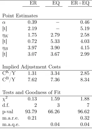
Table 2 reports the point estimates and overall performance of the investment-based model using three different sets of moments conditions in the estimation. In column ER, I only match average stock returns using moment condition (15). In column EQ, I only match average Tobin’s Q using moment condition (16). Finally, in column ER+EQ, I combine the previous two sets of moment conditions.
========================= Insert Table 2 about here
=========================
Table 2 (Point Estimates) shows that the sum of the physical capital and brand capital parameter estimates(αK+αB) ranges from0.39 (only ER used) to0.46 (both ER and EQ
used), which are economically reasonable values (both lower than one as required by a well specified production function).
The estimate of the brand capital adjustment cost parameter ηB ranges from 3.90 to
4.15 and is statistically significant across all sets of moment conditions. The estimate of the capital adjustment cost parameterηKranges from1.75to2.79,and is statistically significant
provided that the Tobin’s Q moments (EQ) are included in the estimation.
18To establish the robustness of the findings, I also tested the model across alternative sets of portfolio
To interpret the magnitude of the estimated adjustment cost parameters, Table 2 (Im-plied Adjustment Costs) reports the average im(Im-plied proportion of firm sales that is lost due to physical capital and to brand capital adjustment costs. These values are computed as CK/Y ≡ 1/2 (ηKIit/Kij)2/Yit for physical capital and CB/Y ≡ 1/2 (ηBAit/Bit)2/Yit for
brand capital. I evaluate these statistics by first computing the portfolio-level time-series of the realized incurred adjustment costs to sales ratio, and then computing the mean of this ratio over time and across all the portfolios.
The estimated magnitude of the physical capital and brand capital adjustment costs is reasonable across all sets of moments. Physical capital adjustment costs range from 1.31% (ER only) to 3.34% (EQ only). These values are well within the lower bound of the empirical estimates surveyed in Hamermesh and Pfann (1996). For brand capital, the adjustment costs are larger. The fraction of sales due to brand capital adjustment costs ranges from 7.36% (EQ only) to 8.34% (ER and EQ). These results highlight the importance of brand capital and brand capital adjustment costs for understanding firm value and stock returns.
Table 2 (Tests and Goodness of Fit) reports three measures of overall performance: the mean absolute return errors in percent per annum (m.a.r.e.), the mean absolute Q errors per annum (m.a.q.e.), and the χ2 test. The m.a.r.e and the m.a.q.e. are computed as the means of the absolute errors across portfolios given by equations (17) and (18), respectively. According to the three metrics considered here, the investment-based model performs very well. The m.a.r.e. ranges from 0.21% (ER only) to 0.32% (ER and EQ). These numbers are small, especially when compared with the large magnitude of the average returns (and spread) of the advertising growth portfolios reported in Table 1: the spread in the returns of advertising growth portfolios is 6.2% per annum, and the average stock returns of the portfolios is 16.9%. The m.a.q.e. are also small, 0.04 across all sets of moments. This pricing error represents less than 2% of the average Tobin’s Q ratio across the portfolios (2.3 as reported in Table 1) and less than 11% of the spread in Tobin’s Q across the portfolios (0.38 as reported in Table 1). Finally, the investment-based model is not rejected by theχ2
5.1.2 Pricing Errors
The m.a.r.e., m.a.q.e., andχ2 tests only indicate overall model performance. To provide a more complete picture, Table 3 reports the stock return pricing error for each portfolio,eSi, as defined in equation (17), as well as the valuation moment pricing error for each portfolio,
eQi , as defined in equation (18). In addition, I report thet-statistic for each individual pricing error, following Liu, Whited, and Zhang (2009). To put the results into perspective, Table 3 also reports the asset pricing test results for traditional asset pricing models such as the CAPM, the Fama and French (1993) three-factor model, and the Carhart (1997) four-factor model on the advertising-growth portfolios. To test the CAPM, I regress monthly portfolio returns in excess of the risk-free rate on market excess returns. The risk-free rate used is the one-month Treasury bill from Ibbotson Associates. The regression intercept (αCAP M) measures the model error for the CAPM. To test the Fama-French model, I regress the portfolio excess stock returns on the monthly returns of the market factor, a size factor, and a book-to-market factor. The regression intercept (αF F3F) measures the error of the Fama-French model. Finally, to test the Carhart model, I extend the Fama-Fama-French model with a momentum factor. The regression intercept (αCAR) measures the error of the Carhart
model. The factor-returns data for the three models is from Kenneth French’s webpage. Finally, to facilitate the comparison across models, I also report the mean absolute error (m.a.e.) for each model, computed as the mean of the absolute alphas across portfolios for each asset pricing model (which I then compare with the m.a.r.e. for the investment-based model).
========================= Insert Table 3 about here
=========================
The basic message from Table 3 is clear: the fit of the investment-based model compares favorably with the fit from the CAPM, the Fama-French model, and the Carhart model. When I use the investment-based model to match expected returns, the m.a.e. of the model is
only0.21% per annum which is considerably smaller than the m.a.e. of the CAPM (4.94%
per annum), of the Fama-French model (3.16%), and of the Carhart model (5.49%). In addition, in contrast with the standard models, none of the pricing errors of each individual portfolio is statistically significant. In particular, the high-minus-low portfolio has a pricing error of only−0.29% (t-stat =−0.36) in the model, which is considerably smaller than the pricing error of −10.06% (t-stat = −4.5) in the CAPM, −8.38% (t-stat = −3.42) in the Fama-French model, and−6.61% (t-stat=−2.70) in the Carhart model.
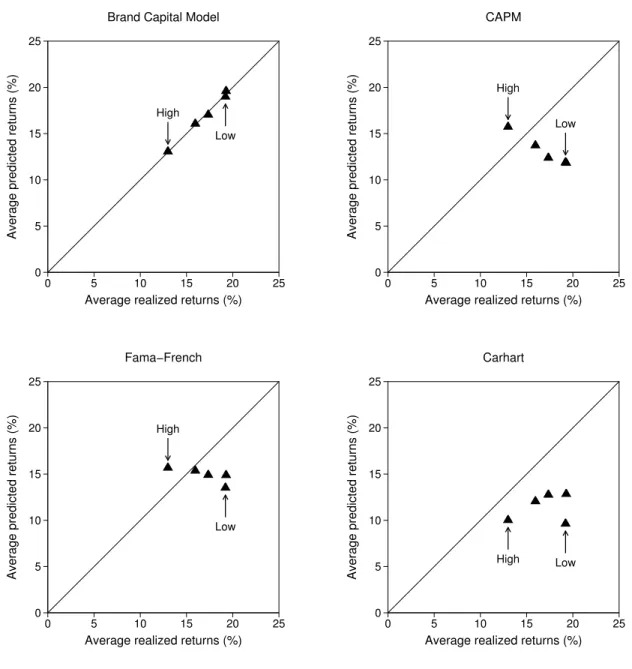
Figure 1 provides a visual description of the good fit of the investment-based model espe-cially when comparing the performance of the model with that from standard asset pricing models. For each model, this figure shows the plot of the average stock returns predicted by the model against the average stock returns of the advertising-growth portfolios in the data. If a model’s performance is perfect, the observations should lie exactly on the 45-degree line. In the top-left panel, the scatter plot of the average predicted returns against the average realized returns of the advertising-growth portfolios is largely aligned with the 45-degree line. The investment-based model’s errors for the individual portfolios (difference from the 45-degree line) are thus small. In contrast, the CAPM, the Fama-French model, and the Carhart model systematically underpredict the expected returns of the advertising-growth portfolios, thus generating large pricing errors. This evidence suggests that, consistent with Liu, Whited, and Zhang (2009), Q-theory outperforms traditional asset pricing models in capturing the cross-section of expected returns.
========================= Insert Figure 1 about here
=========================
Importantly, the fit of the investment-based model compares favorably with the fit of the standard asset pricing models even when the model is estimated to match both expected returns and average Tobin’s Q (standard asset pricing models are not designed to match
in the investment-based model, which is still substantially smaller than the pricing errors of the three alternative asset pricing models. In addition, the m.a.e. for Tobin’s Q moments is only0.04 (or again, less than2%of the average Tobin’s Q across portfolios), and none of the individual portfolio-level Tobin’s Q errors is statistically significant. Figure 2 provides a visual description of the good fit of the investment-based model when matching both average returns and firm value. Clearly, most observations remain well aligned with the 45-degree line across the two set of moments, and thus the model continues to generate low pricing errors.
========================= Insert Figure 2 about here
=========================
6
The Value of Brand Capital
In this section, I use the results from the estimation of the investment-based model to quantify the importance of brand capital for firm value, and relate the findings to the large literature in marketing on brand valuation. As discussed in Section 2, the importance of brand for firm value is well established in the marketing literature. The methodology used in this paper provides a novel way of measuring brand equity grounded in economic theory, thus providing an alternative, yet complementary, approach to the existing methods of measuring brand equity.
6.1 Industry-Level Analysis
Using the model parameters estimated in the previous section, I compute the importance of brand capital for firm value across different industries in the economy. This procedure allows me to quantify not only the importance of brand capital for firm value in the overall economy, but also the extent to which the importance of brand capital varies across industries.
across industries (i.e. the technology parameters are not industry-specific), the value of brand capital may vary across industries due to different physical investment and advertising rates. In turn, this implies that firms in different industries have different physical capital and brand capital stocks (both in absolute terms and in relative terms), and thus that the relative importance of brand capital and physical capital for firm value may vary across industries. For this analysis, I consider the highly disaggregated 48 Fama-French industry classification (see Kenneth French’s webpage for a detailed description of each industry).19
I compute the importance of brand capital for firm value in each industry as follows. Using the firm-value decomposition in Proposition 1, the fraction of firm value that is at-tributed to brand capital (WitB) in each industryiand in each year tis given by:
WitB ≡BQitBit+1/(KQitKit+1+BQitBit+1),
in which KQit ≡ 1 + (1−τt)ˆη2KIit/Kit and BQit ≡ (1−τt) 1 + ˆηB2Ait/Bit
. The charac-teristics Iit, Kit, Ait, and Bit in each industry i are computed by aggregating each firm’s
characteristics to the industry-level, using the portfolio-level aggregation specified in equa-tion (20). The average importance of brand capital for firm value (WiB) in each industry is then obtained as the time-series average of the industry-specific realized WitB. To com-pute this value, I use the point estimates ηˆK and ηˆB obtained from the estimation of the
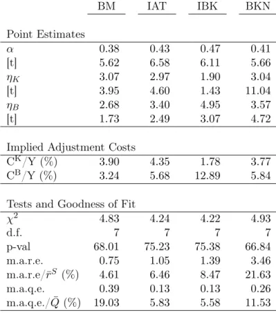
investment-based model on the five advertising growth portfolios reported in Table 2. The results from this analysis are reported in Table 4. In addition, this table reports the average advertising intensity in each industry as measured by the advertising-to-sales ratio and the industry average Tobin’s Q. Advertising intensity is naturally correlated withWiB and helps to understand the extent to which industries differ in their advertising efforts.
========================= Insert Table 4 about here
19
I only report results for 44 industries because 4 industries are eliminated due to missing observations. In addition, I expand the sample size in this analysis by including firms in the Finance and Utilities sectors, and by not excluding firms based on the fiscal-year end.
=========================
The results reported in Table 4 show that brand capital accounts for a substantial fraction of firm market value in most industries, and that this fraction varies significantly across industries. Across all the 44 industries considered here, the mean fraction of firm value attributed to brand capital is about 23%.
The brand value (brand equity) ranges from close to zero for commodities (e.g. Steel, Oil) to about30−60% of firm market value for consumer goods. Note that the industries that produce and sell consumer brand products have much higher-than-average estimated brand equity. In general, the stronger the consumer product orientations, the higher the share of brand capital.
The values reported here are roughly consistent with the values estimated in Simon and Sullivan (1993) using a reduced-form approach, and are in line with the values typically reported in the literature on brand valuation surveyed in Srinivasan, Hsu, and Fournier (2011). This finding suggests that the measure of brand capital that I use has reasonable properties and that the estimation procedure produces reasonable estimates.
6.2 Firm-Level Analysis
In this section, I expand the previous analysis and compute the value of brand capital at the firm-level for the subset of U.S. large firms that report advertising expenditures. This analysis is interesting given the existence of several firm-level rankings published in the aca-demic literature and computed by several consulting firms (e.g. Interbrand, BrandFinance, CoreBrand, among others) which specialize on brand valuation (see the related literature Section 2 for additional references). In turn, this allows me to illustrate the usefulness of the methodology proposed here for practical applications.
The estimated value of brand capital for firmi implied by the estimation results of the investment-based model is obtained directly from equation (7). It is computed as:
Value of Brand Capitalt,i= (1−τt)
1 + ˆηB2 Ait