AN AB INITIO STUDY OF THE STRUCTURAL,
MAGNETIC, AND ELECTRONIC PROPERTIES OF
TRANSITION METAL OXIDES
A Dissertation
Presented to the Faculty of the Graduate School of Cornell University
in Partial Fulfillment of the Requirements for the Degree of Doctor of Philosophy
by Turan Birol August 2013
c
2013 Turan Birol ALL RIGHTS RESERVED
AN AB INITIO STUDY OF THE STRUCTURAL, MAGNETIC, AND ELECTRONIC PROPERTIES OF TRANSITION METAL OXIDES
Turan Birol, Ph.D. Cornell University 2013
Transition metal oxides form a large class of compounds that exhibit a very rich and diverse physics. This thesis involves a first-principles computational study of some transition metal oxides and their different physical properties. We study the emergence of ferroelectricity in Sr-Ti-O layered perovskites with strain, the microscopic mechanism of magnetodielectric coupling in EuTiO3,
and the structural trends of early transition metal dioxides with the Rutile struc-ture. We explain and support the results of our first-principles calculations with physical models for each system.
BIOGRAPHICAL SKETCH
Turan Birol was born in Sivas, Turkey in 1983. He graduated from Ankara Atat ¨urk High School in 2001 and received his BSc in Physics with high honors from the Middle East Technical University with a minor in Logic in 2005. After receiving a MS in Physics from Koc¸ University in 2007, he started his Physics PhD studies at Cornell University. He joined the group of Craig J. Fennie in 2009.
to my parents,
and to the people of my country, with all their good, and all their bad...
ACKNOWLEDGEMENTS
While my original intention was to have a complete list of people to whom I am in debt and the reasons why I am so; I realize that this is practically impossible as such a list would be too long. For this reason, I will not really mention my previous teachers, like Ilksen; or old friends, like Bayram, Kutay, Gizem, Elif, Sarp, or Didem; or any of my role models, such as H.T. Tassadar. I will focus only on the physics and Cornell people.
Of course, I will make an exception for my family, for I guess I have finally reached the age at which one feels that romantic admiration towards his parents. I am unmeasurably thankful for both my parents for doing their best for me. I wish my mother could live to see this day as well - she would probably scold me for still being not-married, but would nevertheless be happy. My brother obvi-ously deserves to be thanked as well: Our noisy and violent quarrels certainly built up character. Hopefully in a good way.
My advisor Craig has been very understanding and helpful about so many things, both professional and personal, during my PhD. I can see many ways that things could have gone bad if I had someone else as my advisor, so I am very thankful to him. I should also thank to various past and present members of the Fennie Group for all the time together. Among them Nicole deserves a separate thank you for the long lunch breaks at CTB, and listening to my endless ranting. I should also not forget to mention Johannes (Herr Doktor).
My physics friends here in Ithaca made this little city so much better than I could ever imagine. In this respect, Stephen, Yj, Shankar, Hitesh, Colwyn, Jolyon, Kendra, Katie, Melina, Ben, and various others deserve a big thank you. The homework sessions, hikes, get-togethers, and even the green man incident were so much fun. The Turkish Mafia at Cornell; including, but not limited to
Erdal, Yucel, Onur, Deniz, Baris, Damla, and Cagatay, also deserve to be men-tioned given how much they helped me feel less home-sick especially in my first years around here. I am also thankful for the Turkish physics gang with whom I have stayed in touch both here on the East Coast and during my visits to Turkey; Cesim, Serkan, Nadir, Can, Sururi, Ziya, and again, various others.
Finally, there are two very special people who have been exposed to me in a way different from everyone else, and deserve a thank you for that. Nora was by my side for a good chunk of my time in Ithaca, and has been extremely supporting and helpful. I am thankful to her for a lot of things, such as getting me used to tofu. April, while she has been around me for only the good part of a year, introduced me to so many new things and contributed to my life in a very positive way. I am still not sure why she bothers hanging out with me, but I hereby thank her all that she has done, including the games she plays with my subconscious mind.
TABLE OF CONTENTS
Biographical Sketch . . . iii
Dedication . . . iv
Acknowledgements . . . v
Table of Contents . . . vii
List of Tables . . . ix
List of Figures . . . x
1 Introduction and Methods 1 1.1 Introduction . . . 1
1.2 Methods . . . 3
1.2.1 Schroedinger Equation for Electrons in the Adiabatic Ap-proximation . . . 3
1.2.2 Density Functional Theory . . . 5
1.2.3 DFT+U . . . 8
1.2.4 The Projector Augmented Wave Method . . . 14
2 Ferroelectricity in Layered Perovskites Srn+1TinO3n+1 17 2.1 Introduction . . . 17
2.2 Methods . . . 21
2.3 Coherence Length . . . 21
2.4 Critical Thickness . . . 22
2.5 Tuning the Coherence Length . . . 24
2.6 The Effect of Rumpling . . . 29
2.7 A Novel Polar State . . . 29
2.8 Auxiliary Material . . . 30
2.8.1 Perpendicular Coherence Length . . . 31
2.8.2 Interplanar Force Constants . . . 34
2.8.3 Transition Temperature Estimate . . . 38
2.9 Comparison to Experiments . . . 42
2.10 Summary . . . 44
3 Why EuTiO3 is not a Ferroelectric and the Microscopic Mechanism of Magnetodielectric Coupling 46 3.1 Introduction . . . 47
3.2 Methods . . . 53
3.3 Results . . . 54
3.3.1 Background . . . 54
3.3.2 An Intriguing Thought Experiment: Polar Mode Fre-quency versus Hubbard-U . . . 56
3.3.3 Magnetic Order Control of Eu-f/Ti-d/O-p Hybridization . 57 3.3.4 The Suppression of Ferroelectricity . . . 60
3.3.5 The Mechanism of Spin-Lattice Coupling and the Origin of Ferromagnetism in Strain-Induced Ferroelectric EuTiO3 65
3.3.6 Oxygen Octahedral Rotations . . . 67
3.4 Summary . . . 70
4 Structural Trends in Transition Metal Dioxides with Rutile and Re-lated Structures 71 4.1 Introduction . . . 72
4.2 Methods . . . 74
4.3 History . . . 76
4.4 The Rutile Structure . . . 78
4.5 Structural Trends of Early Transition Metal Dioxides in the High Symmetry Rutile Phase . . . 81
4.5.1 First-principles Results . . . 81
4.5.2 What Determines c/a, uand How Regular the Octahedra Are . . . 83
4.5.3 Electronic Structure and the M-M Bonding in the High Symmetry Rutile Phase . . . 86
4.6 Cation Pairing . . . 92
4.6.1 Symmetry Analysis of Cation Pairing in Rutile Structure . 93 4.6.2 Instabilities From DFT . . . 97
4.6.3 Mechanism of Pairing . . . 99
4.6.4 Structural Groundstate . . . 101
4.6.5 Is the Pairing Instability Cooperative? . . . 108
4.7 Summary & Conclusions . . . 112 4.8 Appendix: The Baur Distortion Index and The Bond Angle Variance112
5 Conclusions 114
LIST OF TABLES
2.1 Interplanar force constants for the unstrained structure, in units of eV/Å2/ion. Columns denote the ion that is moved, rows
de-note the ion that the force acts on. Layers are listed in increasing distance from the displaced ion, and due to the finite size of the supercell, force constants for atomic layers as far as 3 unit cells are calculated. Subscripts for O’s denote whether they are on a TiO2 or an SrO plane, and OTik denotes the force on the oxygen on the Ti–O chain parallel to the displacement direction, OTi⊥ de-notes the other oxygen on the TiO2 layer. The force constants
presented are symmetrized. This process ensures that all theC(n)
matrices are perfectly symmetric (the symmetrization changed the lowest eigenvalues no more than∼ 1%). . . 40 4.1 Low temperature experimental structures of the dioxides of the
4d and 5d transition metals from 4th to 9th
groups; i.e. with 0 to 5 electrons in the outer d orbitals of the M4+ cation. By
’High Symmetry Rutile’ we refer to the rutile structure with no symmetry lowering structural distortions. Data taken from Ref. [25, 27, 137, 138, 149, 148]. . . 73 4.2 Baur distortion indices and bond angle variances of fully
re-laxed TcO2for different groundstate structure candidates.
Space-groups I41md and P¯421m have two inequivalent octahedra - the
LIST OF FIGURES
2.1 (Inset) The Ruddlesden-Popper, Srn+1TinO3n+1, homologous
se-ries showing two possible polarization directions: in-plane, Pk, and out-of-plane, P⊥. (Main figure) Calculated in-plane polar phonon frequency as a function of n for a fixed in-plane lattice constant of SrTiO3. (Dots are first-principles calculations, curve
is a fit to a single exponential.) . . . 20 2.2 Phonon dispersions of SrTiO3 in its cubic (Pm¯3m) phase at (a)
experimental volume, and under (b) 0.6 % and (c) 1.7 % isotropic tensile strain with respect to the experimental lattice constant. The corresponding ω2 = 0 isosurfaces are shown next to each
phonon dispersion curve. . . 25 2.3 The ω2 = 0 isosurfaces for SrTiO
3 under (a) 0.0%, (b) 0.5%, (c)
1.1%, and (d) 1.7% biaxial strain. Right panels show the cuts of the isosurfaces on kz = 0 planes. For (c) and (d), the slight anisotropy on the surfaces of DyScO3and GdScO3substrates are
taken into account, however, this anisotropy gives barely visible results. . . 27 2.4 (a) Ruddlesden-Popper, (SrTiO3)n(SrO): In-plane polar soft
mode frequency squared versus layering number n. (b) Per-ovskite Slab Model, (SrTiO3)m: Lowest in-plane polar
interpla-nar force constant matrix eigenvalue versus thickness of SrTiO3.
Strain values are given with respect to the lattice constant of SrTiO3. The slab thickness in panel b, given in number of SrTiO3
layers, corresponds to half the number of atomic SrO or TiO2
lay-ers in the slab. Half integer values correspond to an odd number of atomic layers that are terminated by TiO2 layers o both sides.
Similar calculations for slabs terminated by SrO layers, not pre-sented here, give qualitatively similar results even though the force constants are higher for small thicknesses. The lines are fits to exponentials. . . 28 2.5 Sr4Ti3O10 ground state under 1.1% tensile strain. (a) Schematic
of ferroelectric (FE) and antiferroelectric (AFE) distortions. (b) Rumpling distortion (defined as the distance along [001] be-tween cations and oxygens on the same layer). (c) Energy gain due to FE and AFE distortions in structures with rumpling. (d) The same as (c) except the rumpling distortion has been artifi-cially set to zero. . . 31 2.6 Displacement patterns for the branch stemming from the FE
mode for various wave vectors. Each arrow represents the local polarization direction (direction which the cations are displaced) of a single primitive unit cell. . . 33 2.7 First Brillouin zone for bulk SrTiO3in space group Pm¯3m. . . 34
2.8 Projection of one of the disks in Figure 2a of main text on the
qx–qzplane. . . 35 2.9 The 1 × 1 × 6 perovskite supercell and 3 of the 5 inequivalent
displacements used to calculate the IPFCs. Green spheres corre-spond to Sr ions, blue ones to Ti ions, and red ones to O ions. . . 39 2.10 Energy gain, per formula unit, of the ferroelectric mode forn= 1
ton = 5RP phases under different strain states. The horizontal dotted line corresponds to the energy gain per formula unit of SrTiO3under1.1%tensile biaxial strain. . . 41
2.11 Experimental results for dielectric properties of Sr-Ti-O RP com-pounds. (a) Real part of the in-plane dielectric constant of films deposited on DyScO3 substrate, as a function of temperature at
different frequencies. (b) Critical temperatureTc of the films de-posited on DyScO3and GdScO3substrates. Tcis calculated from the position of the dielectric constant peak at 1 MHz. Error bars give a measure of the variation of Tc in separately grown sam-ples. (d) Remanent polarization at 10 K of the films on DyScO3.
Inset: Polarization hysteresis loops at the same temperature. (Figure reproduced from [100].) . . . 43 2.12 Energy (per n) of the Sr-Ti-O RP compounds as a function of
polar displacement amplitude in the (001) plane. For all com-pounds, the minimum energy is obtained with polarization alongh110idirections. (Figure reproduced from [100]. . . 45 3.1 (a) Crystal structure of perovskite EuTiO3in the cubic phase. (b)
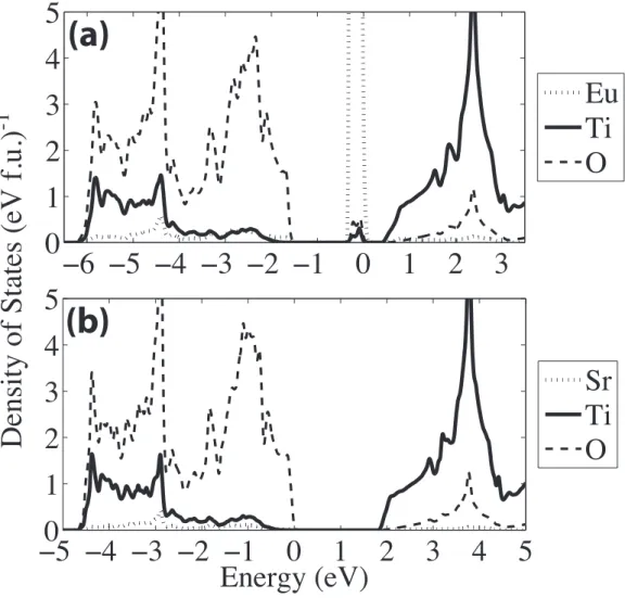
Sketch of G-type antiferromagnetic order. Arrows denote the di-rection of spins. . . 49 3.2 (a) Density of states (DOS) of EuTiO3, calculated from
first-principles. (b) DOS of SrTiO3, calculated from first-principles.
The zero points of energy in the DOS plots are aligned with the highest occupied level. . . 52 3.3 Polar soft-mode frequency, ωS M, vs. the on-site interactionUEu
on Eu 4f orbitals. Red squares and blue asterisks denote the fre-quencies calculated in AFM and FM states respectively. . . 55 3.4 Two examples of maximally localized Wannier functions of Eu f
electrons in EuTiO3. (a) fzy2 ∼z(4y2−z2−x2), (b) fxyz ∼ xyz. Yellow
and green parts of the Wannier Function correspond to isosur-faces of opposite sign, and the Europium ion is in the center of the cubic cell. . . 57 3.5 Charge on Ti d orbitals due to hybridization of the Eu f states
(σT i) versus Hubbard-UEu used in DFT+U calculations. Red squares and blue asterisks denote values in AFM and FM states respectively. . . 59
3.6 The Eu fxyzMLWF for different values ofUEu. For simplicity, the oxygen ions are not shown on the figure. . . 60 3.7 (a) Sketch of the fxyz orbitals on3rd neighbor Eu ions and the
in-termediate Ti ion’sd(x+y+z)2 orbital. (b) Energy levels of the three
orbitals in the FM state. Lowest lying excitations where an elec-tron hops onto the Ti cation, (c) and (d), are allowed, but not both the electrons can hop at the same time because of Pauli ex-clusion (e). However, in the AFM state, (f), not only the lowest excitations (g) and (h) but also the correlated hopping sketched in (i) is allowed. . . 61 3.8 Self force constants (C˜) for the fourΓ point symmetry adapted
modes (left) and the corresponding displacement patterns (right). Red squares and blue asterisks denote the force constants in AFM and FM states respectively. . . 64 3.9 Self force constant of Ti ion (C˜T i) as a function of σT i (the charge
on Ti d shell due to hybridization with Eu f states). Red and blue curves denote values calculated in AFM and FM states respec-tively. Black line is a best fit to the data. Note that the data on this plot can be extracted from Fig. 3.5 and 3.8. . . 67 3.10 (a) R point rotation soft mode frequency as a function ofUEu in
the FM and the AFM states and the cubic structure with lattice constant fixed to 3.90 Å. The horizontal black line corresponds to the soft mode frequency in SrTiO3, calculated with the same
settings. (b) Octahedral rotation angle, obtained by relaxing the ions in fixed cubic cell, as a function of UEu in the FM and the AFM states. The horizontal black line corresponds to the rota-tion angle in SrTiO3, calculated with the same settings. Lines
connecting the data points are provided to guide the eye. . . 69 4.1 The Rutile structure. Red spheres represent oxygens, and blue
spheres represent metal cations. (a) The primitive unit cell, which contains two formula units. Each metal ion is sur-rounded by six oxygens, and each oxygen makes bonds with three cations. (b) The corner-sharing octahedron network, as seen from [001] direction. (c) Oxygen octahedra form edge shar-ing chains in the [001] direction. (d) The metal-oxygen network as seen from [100] direction. . . 79
4.2 Structural parameters from first-principles calculations for the TM dioxides in hugh symmetry Rutile phase as a function of the number of d electrons on the M4+cation. (a) In-plane lattice
constant a. (b) c/a ratio; i.e. the ratio of in-plane and out-of-plane lattice constants. (c) The anion parameter u. (d) Volume of the primitive unit cell. Red and blue data correspond to 4d and 5d compounds respectively. Horizontal, dashed black lines correspond to the values ofc/aanduin the ideal Rutile structure, i.e. when the oxygen octahedra are regular. . . 82 4.3 Effective ionic radii for transition metal ions in the 4+
oxida-tion state, as a funcoxida-tion of the number of d electrons on the M4+
cation. Red and blue data correspond to 4d and 5d cations re-spectively. (Data from Ref. [116].) . . . 83 4.4 (a) Baur Distortion Indices and (b) Bond Angle Variances for TM
dioxides in the high symmetry Rutile structure as a function of the number of d electrons on the M4+ cation. Red and blue data
correspond to 4d and 5d cations respectively. . . 84 4.5 The anion parameter u as a function of the number of d
elec-trons on the M4+cation; (a) obtained from ionic relaxations, and
(b) calculated from usingc/athrough Eq. 4.1. Red and blue data correspond to 4d and 5d cations respectively. Horizontal, dashed black lines correspond to the value ofuin the ideal Rutile struc-ture, i.e. when the oxygen octahedra are regular. . . 87 4.6 (a) Sketch of the Metal-Oxygen angles in the ideal Rutile
struc-ture. (b) The Metal-Oxygen-Metal angles in the TM dioxides in the high symmetry Rutile structure as a function of the number of d electrons on the M4+ cation, from first-principles. Red and
blue data correspond to 4d and 5d cations respectively. The hor-izontal lines drawn at 90◦
and 135◦
correspond to the angles in the ideal Rutile structure. . . 88 4.7 Sketch of the angular part of the transition metal d orbitals’
charge densities. (The choice of axes and their naming follow Ref. [48, 68].) The red and blue atoms represent oxygen and metal ions respectively. . . 89 4.8 Sketch of the angular part of the charge densities of the three
d orbitals which have overlapping lobes with the other metal cations. Red and blue atoms represent oxygen and metal ions respectively. . . 91 4.9 High symmetry q-points in the first Brillouin zone of simple
4.10 Sketches of the cation pairing patterns corresponding to A1, R+1,
and Z1 irreps, and also the cation displacement pattern
corre-sponding to the Γ−
3 irrep. Red circles represent oxygens, blue
circles represent metal cations. For A1, R+1, and Z1 irreps, there
are multiple possible directions, but only the high symmetry di-rection which gives the lowest energy is sketched in this figure. Also, only the cation pairing displacements are shown, and the displacements of the other symmetry adapted modes, such as oxygen displacements, are omitted for simplicity. . . 95 4.11 Unstable modes of the high symmetry Rutile structure and
pos-sible groundstates they can lead to. Only the subgroups that can be reached in a 4 formula unit supercell are listed. The MoO2
structure P21/cis obtained by the irrep R+1 along(a,0,a,0)
direc-tion. . . 96 4.12 Force constants matrix eigenvalue of the normal modes with the
largest cation pairing components for (a) A1, (b) R+1, (c) Z1
ir-reps. (d) The force constants matrix eigenvalue for the optical
Γ−
3 mode. The red and blue data correspond to 4d and 5d cations
respectively. . . 97 4.13 Energies of structures in different spacegroups with respect to
the nondistorted Rutile structure. The normal modes and the spacegroups that they lead to are given at the legend. (a) Results of full geometric relaxations, which include the optimization of the cell shape and volume as well as the ion coordinates. (b) Results of relaxations made with fixed lattice vectors. . . 103 4.14 (a) Pairing amplitude vs. energy gain for wavevectorsR(green),
A(blue) andZ(red). The data points are from first principle cal-culations, and the dashed lines are a 6th order fit to the data. Amplitude of pairing is given in terms of the lattice constant a. (b) Curves are the same as (a). The circles correspond to the en-ergy gain and pairing amplitude for the structures with relaxed ionic coordinates in the spacegroups with R+1 (green), A1 (blue),
and Z1(red) modes frozen in. . . 105
4.15 (a) Local cation pairing distortions with n = 1 (left) and n = 2 pairs of cations along the edge-sharing chains being displaced. The calculations are performed in a1×1×1supercell, as a result, the displacements have~k = (0,0,32πc). (b) Self force constants of cation pairing displacement with respect to the number of cation pairs displaced along the[001]direction (n). . . 111 5.1 Number of publications in the Web of Knowledge that have
’transition metal oxides’ as their topic. Data is obtained by aver-aging citations in two consecutive years. . . 115
CHAPTER 1
INTRODUCTION AND METHODS
1.1
Introduction
Understanding the behavior of electrons in solids has been a major challenge for the physics of the 20th and the early 21st centuries. Even though the fundamen-tals of the quantum theory were established in 1920s, and calculations on the electrons in atoms were attempted immediately (for example see [77, 76, 44, 73]), the electronic structure of solids still provide open problems to this date. While a detailed review of the complexity of these calculations is beyond the scope of this brief introduction, it is possible to justify the growing interest on them by the richness of new physics that emerges at different scales. We can summa-rize this in one sentence by the famous motto of solid state physics: ”More is different” [5].
Transition metal (TM) oxides is a class of materials that have been in the fo-cus of intense research in the fields of Physics, Chemistry, and Materials Science for almost a century now. They exhibit a very wide range of interesting phenom-ena; of which ferroelectricity, multiferroicity, metal-insulator transitions, and high temperature superconductivity are just a few. As a result, the amount of research effort focused on TM oxides and the various orders observed in these systems (including, but not limited to, various structural (ferroelectric, ferrodis-tortive, antiferrodisferrodis-tortive, etc.) as well as different magnetic and orbital orders) is increasing every day. The interplay of these phenomena render the TM oxides a uniquely rich playground for solid state physics.
Both the development of advanced techniques and increasing computer power lead to a surge of computational studies on TM oxides. State of the art first principles methods provide a powerful arsenal to approach the physics of TM oxides, and can be used not only to support and explain experimental re-sults but also to make predictions and guide the experiments. Even though the necessary basic physical laws are known, as discussed above, these methods provide new physical understanding about the complex emergent physics of TM oxides.
This thesis involves a study on the TM oxides and part of the rich physics they host from a computational theory perspective. It consists of three main parts, each of which focus on a specific compound or group of compounds that exhibit a different phenomenon. They are:
• A study of the strain-tunability of ferroelectricity in Sr-Ti-O Ruddlesden-Popper compounds, and a novel polar state that emerges because of the competition of ferroelectricity with antiferroelectricity in them [23]. This part is an example of how the first-principles approaches can be used to study the structural instabilities and phase transitions in TM oxides.
• A study of the microscopic mechanism of the magnetoelectric coupling in EuTiO3, the effect of rare earth f electrons on the dielectric properties
and crystal dynamics in this compound, and the connection between the oxygen octahedral rotations with magnetism and ferroelectricity [83, 143]. This part shows how first-principles approaches provide unique capabil-ities to perform thought experiments that probe the microscopic mecha-nisms behind the macroscopic properties of materials.
rutile structure, and their connection with the electronic structure. It in-volves a detailed study of a large number of compounds and performing calculations that isolate certain properties, such as the coupling of struc-tural distortions to strain, which is not possible to achieve without use of computational methods.
The method that has been used throughout these studies is the Kohn-Sham Density Functional Theory [109]. We start by providing a very brief background on our methods in Section 1.2. We then present our studies on the ferroelectric-ity in SrTiO3, the multiferroicity in EuTiO3and the structural trends of the rutile
compounds in Chapters 2, 3, and 4 respectively. Conclusions are in Chapter 5.
1.2
Methods
In this section we give a very brief background on the methods that we use. A very good discussion of almost everything in this section is present in the manuscript of Martin (Ref. [109]).
1.2.1
Schroedinger Equation for Electrons in the Adiabatic
Ap-proximation
The basic Hamiltonian that governs the physics of electrons interacting with atomic nuclei is H = −X ~ 2 2m ∇ 2 i − X ZIe2 ~ ~ + 1 2 X e2 |~r −~r |− X ~2 2M ∇ 2 I + 1 2 X ZIZJe2 ~ ~ (1.1)
where small latin indices refer to the electrons, capital latin indices refer to the nuclei,~randR~are the positions of the electrons and the nuclei,meis the mass of the electron, MI andZI are the masses and charges of the nuclei,eis the charge of the electron, and~is the Planck’s constant [109]. The wavefunctionΨ of the
system is a function of the positions of both the electrons and the nuclei, and is in general not seperable in them; i.e. the electronic and nuclear degrees of freedom can be entangled. However, since the nuclear mass is much larger than the electronic one, there is a separation of scales. As a result, we can make the approximation
Ψ = Ψe·Ψn (1.2)
where the electronic wavefunctionΨe is a function of only the electronic coordi-nates, and the nuclear wavefunctionΨn is a function of only the nuclear coordi-nates. This is the first step of the so called Born-Oppenheimer approximation. It results in an electronic Schroedinger equation that has the form
HΨe = EΨe (1.3) = −X i ~2 2me ∇2i + 1 2 X i,j e2 |~ri−~rj| +Vext Ψ e (1.4)
whereEis the energy eigenvalue andVextis the external one-body potential that the electrons feel:
Vext(~r)=X I
ZIe2 |~r−R~I|
(1.5)
A further approximation that is commonly made is to consider the nuclei as classical particles that are stationary, and assume that the electrons are always in their ground state. In this regime, solving Eq. (1.3) for the groundstate for fixed nuclear coordinates solves the problem completely. The force on theIth
nucleus can then be calculated using the Hellmann-Feynman theorem [54] in terms of the nucleus-nucleus Coulomb energyEnnand the total electronic charge density
n(~r)as ~ FI =− ∂Enn ∂~RI − Z d3rn(~r)∂Vext(~r) ∂~RI (1.6)
Phonon frequencies can be calculated from Eq. (1.6) by defining interatomic force constants as
CIαJβ =− ∂FIα ∂RJβ
(1.7)
and solving the Newton’s equations for the nuclei, in the so called Born-von Karman fashion [105, 28]. (The greek indices denote cartesian components.)
This adiabatic approach to phonons can and does indeed fail in two lim-its. Even tough the nuclear masses are much larger than the electronic one, the quantum fluctuations in the positions of the nuclei can nevertheless be impor-tant for lighter nuclei, and also for systems with optical phonons with a small frequency, in other words, systems on the verge of a structural phase transi-tion (for example see [176] and the discussions in Chapters 2 and 3). Also, the approximation that the electrons remain in their groundstate requires that the atomic motion is not rapid enough to excite electrons, i.e., the typical phonon frequencyωis smaller than the electronic gapEg,~ω Eg. However, for metals,
Egis vanishing, and so phonons decay after a finite lifetime [131]. Nevertheless, the Born-von Karman approach to lattice vibrations provides valuable insight into the lattice dynamics if retardation effects are ignored, and into the structural phase transitions if quantum fluctuations of the nuclei is not significant.
1.2.2
Density Functional Theory
The Hamiltonian of the electrons in a crystalline solid, and the Scroedinger equation which determines the electronic wavefunction is presented in Section
1.2.1. In the words of Dirac, ”The general theory of quantum mechanics is now al-most complete. The underlying physical laws necessary for the mathematical theory of a large part of physics and all of chemistry are thus completely known”[45]. However, the electronic wavefunctionΨeof anNelectron system is a complex function of 3N coordinates, and as a result, is not easy to handle. So, actually solving Eq. 1.3 and obtaining the wavefunction for interacting electrons is not trivial, and in many cases, not even possible.1
An approach that can be traced back to the early days of quantum mechanics is to work with the total electronic densityn(~r)instead of the many-body wave function [163, 53].n, being a real function of only three variables, is much easier to handle thanΨe. Nevertheless, the original density functional formulation of Thomas and Fermi is far from being precise enough for a practical calculation. The crucial steps that made a density functional theory (DFT) applicable to real systems were taken by Hohenberg, Kohn, and Sham in 1960s. In Ref. [79], Hohenberg and Kohn proved two important theorems (reproduced here from Ref. [109]):
• ”For any system of interacting particles in an external potential Vext(~r), the potential Vext(~r)is determined uniquely, except for a constant, by the ground state particle densityn(~r).”
• ”A universal functional for the energy E[n] in terms of the density n(~r) can be defined, valid for any external potentialVext(~r). For any particular
Vext(~r), the exact ground state energy of the system is the global minimum value of this functional, and the densityn(~r)that minimizes the functional is the exact ground state density.”
1We emphasize that this is not a practical matter only, but rather an issue of exponential
These Hohenberg-Kohn theorems prove that for the groundstate, an exact den-sity functional theory can be built. However, obtaining the exact functionalE[n] is no easier than solving for the many-body wavefunction Ψe: the Hohenberg-Kohn theorems prove only the existence - they do not provide a way to solve for it. In order to solve for density n and the energy, Kohn and Sham came with an ansatz that replaces the original interacting system with a noninteract-ing system that has the same groundstate densitynbut under another external potentialVext[88]. The Hamiltonian for this auxiliary system is
Haux= − 1 2∇
2+
VKS(~r), (1.8)
and the density is given by a sum over the occupied orbitals
n(~r)= X i
|φi(~r)|2. (1.9) The kinetic energy part, in terms of the orbitalsφi, is given by
TKS =− 1 2 X i hφi|∇2|φii. (1.10)
We also define the Hartree energy as the Coulomb energy of a classical system with densityn(~r) EHartree = 1 2 Z d3r1 Z d3r2 n(~r1)n(~r2) |~r1−~r2| (1.11)
Putting these together, the ground state energy can be written as
EKS =TKS + Z
d3rVext(~r)n(~r)+EHartree[n]+Exc[n]. (1.12) The quantum many-body effects in the form of exchange and correlation ener-gies are included inExc. Taking the derivative ofEKS with respect toφi(~r)gives the Kohn-Sham potential in Eq. (1.8) as
VHartree(~r)= δEHartree
δn(~r) , (1.14)
Vxc(~r)= δExc
δn(~r). (1.15)
The Kohn-Sham wavefunctionsφi, energy, etc. can be obtained by solving Eq. (1.8)-(1.15) self consistently. However, in order to have an exact theory, the form of Vxc needs to be known. While this is not the case, there are multiple ap-proximations to Vxc. Some examples are the so called Local Density Approxi-mation (LDA) or various Generalized Gradient ApproxiApproxi-mations (GGAs). These approximations introduce errors in the calculated ground state properties, and as a result they should be used with caution. For example, LDA is known to un-derestimate volumes in solids by few percent, which can have dramatic quanti-tative effects on the dielectric properties of oxides. Nevertheless, very often, the use of an approximateVxcis justified by the small errors and the computational ease.
1.2.3
DFT+U
LDA performs surprisingly well in various compounds, and it gives very ro-bust results especially for crystal structure and dynamics. However, despite its success, there is also a tremendous range of materials that it fails in and phys-ical properties that it cannot reproduce. An example is the strongly correlated materials that have ions with partially filled d or f shells. For example, it has been noticed early on [42] that while LDA reproduces the lattice stability for the parent compound of high-Tc oxide superconductors correctly, it often predicts
them to be metallic. However, these compounds are antiferromagnetic insula-tors. There are numerous other examples; even the simple electronic structure
of classical oxides such as MnO or NiO, which are antiferromagnets, cannot be reproduced by LDA correctly [125], and LDA predicts them to be nonmagnetic.
These issues are not essentially problems of DFT but rather that of LDA. While DFT is exact, LDA is not, and it is problematic especially in situations that are far from the homogenous electron gas which is the starting point of LDA. In particular, the derivative discontinuity of the energy [129] does not ex-ist for the homogenous electron gas, so LDA or simple GGAs cannot reproduce this discontinuity. At this point, one can consider abandoning LDA altogether and resorting to advanced methods such as configuration interaction. Another approach is to consider extensions of DFT that correct for shortcomings of LDA. An example is the so called Self Interaction Correction (SIC) method [81, 109], which involves canceling the nonphysical interaction of the electrons by them-selves in the DFT+LDA scheme. There are also the Hybrid Functionals which add some exact Hartree-Fock exchange [15, 128]. However, these methods all bear enormous computational cost.
In this work, we use only a simple yet robust method, DFT+U, which is an extension of DFT+LDA with virtually no extra energy cost. While it has short-comings of its own, DFT+U provides significant improvements over LDA in various properties and systems. In particular, it predicts the correct groundstate for the aforementioned systems like MnO. The major reason that LDA fails in re-producing the magnetic state in these systems is that it cannot take into account the strong Coulomb interaction of localized electrons in systems such as Mott insulators. The magnetism in a homogenous electron gas is due to the exchange interaction between delocalized electrons and can be explained by the Stoner physics. While LDA can properly describe the Stoner physics, it fails to
repro-duce the correlated physics of the Hubbard-like terms that is the driving force of spin (and orbital) polarization in various insulating transition metal oxides [7, 46]. This strongly correlated physics, however, is known to be explained well with Hamiltonians like the Hubbard or Anderson impurity models. DFT+U is a (static) mean field method that introduces the Hubbard physics of the strongly correlateddor f orbitals to the DFT+LDA calculations. The particular flavor of DFT+U we use involves adding a potential to the atomicdor f orbitals [7]:
Vmσ =U X m0 nm0,−σ−n0 +(U− J) X m0 ,m nm0σ−n0 . (1.16)
Here, the sums are over the local (atomic-like) orbitals which have occupations
nmσ, and average occupation n0. σ denotes the spin. It is possible to calculate the two undetermined parametersUandJfrom first-principles [96], or they can be fitted to experimental measurements of a quantity of interest. In either case, scanning a range ofUandJvalues to check for robustness of the physical results is necessary. Also, there is arbitrariness in the choice of the orbitals that this potential is added to, which is a shortcoming of the DFT+U method as presented in Eq. 1.16. However, there are ways to overcome this issue and achieve basis set independent realizations of DFT+U [103].
Physically,Ucorresponds to the Hubbard parameter, which adds an energy cost of occupying a state that is proportional to the total occupation of all the other states. This way, it makes up for the strong Coulomb repulsion between electrons occupying these states. Screening effects should be taken into account when determining the quantitative value ofU since thes-p, d-setc. transitions are faster than thed or f electrons’ fluctuations and hence can screen them [7]. (This latter fact also justifies the applicability of model Hamiltonians with only few local degrees of freedom to such systems.) One usually uses aU that is no larger than ∼ 6− 8eV for 3d electrons, and even smaller values for the lower
rows of the periodic table, which are much smaller than the atomic values. Jcan be associated with the Stoner parameter which aligns spins in different orbitals. It adds an energy gain for occupying parallel spin states. Its typical energy scale is much smaller than U and is less than ∼ 1 eV. While the quantitative value of J is usually considered not to be as important as U, there are studies that underline its significant effects, for example in noncollinear magnetic systems [30].
Note that in the Hubbard hamiltonian for a single site,
E ∼U X
m,σ,m0,σ0
nmσnm0σ0, (1.17)
the spin and orbital polarizations are treated on equal footing. Since it is ener-getically favorable to concentrate occupation on as few states as possible, orbital polarization is induced as well as the spin polarization [7]. This improves the properties of Mott insulators in DFT since an orbital polarization is necessary to open a Mott-Hubbard gap away from half filling of thed or f orbitals [103]. Orbital polarization is also necessary for the orbital ordering observed in Jahn-Teller compounds such as KCuF4. These compounds displays a crystal structure
that goes along with an ordering of the occupation ofd orbitals on the Cu ion. It is shown in [103] that LDA fails to reproduce both the orbital order and the crystal structure, but LDA+U predicts the correct crystal structure, as long as orbital polarization is allowed. (Note that for this type of calculations the basis set independence of the particular DFT+U formulation used is essential, since the electronic structure itself is required to break the orbital symmetry.)
The DFT+U method also reintroduces the derivative discontinuity of the energy functional that is missing in the LDA (or GGA) form of the
exchange-ternative DFT+U formulation due to Dudarev et al. [46] which is rotationally invariant and involves adding the following term to the Kohn-Sham energy:
EDudarev = Ue f f 2 X m,σ nm,σ−n2m,σ . (1.18)
This introduces an energy cost that is vanishing when total number of electrons
N is integer. Near integer N, EDudarev is linearly increasing for both increasing and decreasing N, which creates a kink and hence a derivative discontinuity. The derivative discontinuity is missing from LDA because it approximates the convex, piecewise linear energy functional with a smooth function. The dis-crepancy between the real functional and the LDA approximation is minimum for integerN and as a resultEDudarev tries to make up for the difference between them. (For a pedagogical exposition of this point, see the discussion and Fig. 3.1 in [39].)
Adding a term that favors integer occupation to the Hamiltonian obviously can change the hybridization of an atom with others as well. This, in turn, can lead to changes in covalent bonding and the quantitative features such as Born Effective Charges [62] and the value of electronic contribution to electric polar-ization. While it is not argued explicitly in the literature, LDA tends to over-estimate the electronic contribution to polarization. For example, it has been noticed more than a decade ago in [62] that the polarization of BaTiO3
calcu-lated from Born Effective Charges from LDA is about ∼ 30 % larger than the experimental value even when the experimental lattice structure is used in the calculations. It can be argued that the shortcomings of LDA about the correla-tions on the B-site Ti atom’sdorbitals makes it easier for the O atoms’ occupied
pstates to hybridize with the Ti ion, thus making it less costly for charge to be transferred from O to Ti ion when polarization sets in, increasing the Born Ef-fective Charges and hence the polarization. The results of our calculations (not
shown) indicate that using the LDA+U formalism and adding a Hubbard-U to the Ti d orbitals indeed decreases the anomalously large effective charge of Ti ion thus reproduces a polarization that agrees better with experiment. An ex-treme example of a similar case is the improper ferroelectric HoMn2O5, which
has a large electronic polarization that is induced by the symmetry breaking by the collinear antiferromagnetic order and the resulting spin-dependent hy-bridization [64]. It is shown in [64] that depending on the value ofU used, the polarization in the same crystal structure is not only ’decimated’ but can even change sign. LDA+U also corrects the overestimation of polarization in the sim-ilar compound TbMn2O5[36].
We conclude our discussion of DFT+U method by briefly mentioning some alternatives to it. A commonly used alternative is the hybrid functionals, which involve adding a fraction of exact Hartree-Fock exchange to the LDA exchange correlation energy (for example, see [122]). This cancels some of the exchange interaction of the electrons by themselves, and as a result lead to improve-ments. Hybrid functionals have been extensively used for TM oxide systems, are shown to give good results for, for example, the spin-phonon coupling in various compounds [80, 3]. The insulating phase of VO2, which cannot be
re-produced by DFT+U, is predicted correctly by the Hybrid functionals thanks to the nonlocal nature of the exact exchange added [49]. However, the com-putational cost of Hybrid functionals, while spanning a wide range depending on the formulation, is significantly larger than DFT+U. There exist meta-GGA’s [160], which are significantly cheaper than hybrid functionals. They involve an exchange-correlation energy that depends not only on the density and its gra-dient but also on the kinetic energy density. While they have found widespread use in chemistry literature, the use of meta-GGA’s in physics community is not
wide spread so far. (For example, the study on the implementation of meta-GGA’s in a Projector Augmented Wave framework, Ref. [159], has accumulated only five citations in about two years.)
In summary, DFT+U has proven very successful for various TM oxide sys-tems despite its simplicity. It bears no extra computational cost on top of DFT, and is easy to implement. As a result, it is now implemented in pretty much all widespread DFT packages. There exist other methods, such as Dynamical Mean Field Theory which includes and goes beyond DFT+U; however, the low computational cost associated with DFT+U, as well as its simplicity that renders the results easy to analyze, makes it a very useful and popular tool.
1.2.4
The Projector Augmented Wave Method
In this section, we very briefly introduce the Projector Augmented Wave (PAW) method, which is used to make the numerical DFT calculations more feasible. Throughout the work presented in this thesis, the PAW method as implemented in the Vienna Ab initio Simulation Package (VASP) is extensively used. Further details of the method and comprehensive discussions of it can be found in [24, 109].
In real materials, the wavefunctions of the electrons exhibit very different characteristics near the atoms than they do far from them. Near the atoms, the wavefunctions oscillate very rapidly, and atomic orbitals form a suitable basis to expand them. In the space between the atoms, on the other hand, the wavefunc-tions are more easily expanded in terms of planewaves. The PAW method pro-vides both a means to describe the wavefunctions with high accuracy, and also
a degree of freedom that can be used to choose a computationally convenient basis. In the PAW formalism, the space is divided into two parts: in the so-called augmentation region (Ω) near the atoms, the wavefunctions are expanded in the atomic orbitals, whereas outside the augmentation region planewaves are used for the same purpose. On the boundary ofΩ, boundary conditions are imposed to match the two expansions and their derivatives.
The PAW formalism also involves transforming the physical wavefunctions |Ψi to wavefunctions in a pseudo (PS) Hilbert space |Ψ˜i by a linear operator: |Ψi = T|Ψ˜i. The PS wavefunctions|Ψ˜iare equivalent to to |Ψioutside the aug-mentation region but differ from them inside it. Expectation value of any oper-ator Aˆ can be calculated using the PS wavefunctions as hΨ|A|Ψi = hΨ˜|T†ATˆ |Ψi. SinceΨandΨ˜ differ only the augmentation regionΩ,T is equivalent to identity outsideΩand hence it can be written as
T = 1−X
i
(|φii − |φi˜i)hp˜i|. (1.19)
Here,|φiiand|φi˜ iare thepartial wavesthat are used to expand the wavefunctions in the physical and PS hilbert spaces respectively, andhp˜i|are theprojector func-tionswhich are localized inΩ. The partial waves in the two spaces have a one to one correspondence, i.e.
|Ψ˜ii= X i ci|φi˜i, (1.20) and |Ψii= X i ci|φii (1.21)
with the same coefficientsci =hp˜i|Ψ˜i.
An advantage of defining the projectors and working in the PS Hilbert space is that the operators are invariant under the addition of another operator of the
form
ˆ
B−X
i,j
|p˜iihφi˜ |Bˆ|φ˜jihp˜j| (1.22)
with Bˆ localized in the augmentation region. This freedom can be exploited to remove the singularities like the one that the Coulomb interaction has near the origin. This renders the results less sensitive to energy cutoff of the plane waves, making numerical calculations less costly. As we do not make any development of the PAW formalism but only use it as implemented in publicly available soft-ware packages, we do not elaborate further and refer to the literature for details of it [24, 94, 109].
CHAPTER 2
FERROELECTRICITY IN LAYERED PEROVSKITES Srn+1TinO3n+1
In this chapter, we study the quantum paraelectric SrTiO3 and the closely
related compounds Srn+1TinO3n+1 with the Ruddlesden-Popper (RP) structure
[23, 140, 141]. The RP compounds provide a extra degree of freedom to the perovskite structure: the layering (n). We analyze in detail how a ferroelec-tric instability emerges with increasingnand strain, and provide a model that explains the ferroelectric soft-mode behavior and is consistent with the first-principles calculations. We also predict a novel polar state which involves de-generate ferroelectric and antiferroelectric states in these materials. Finally, we briefly compare our results with experimental observations.
Understanding the ferroelectric behavior of the Sr-Ti-O RP compounds is important because these materials can be tuned to the verge of a parelectric– ferroelectric transition to achieve a large dielectric response. Also, they are ob-served to accommodate nonstoichiometry by shear planes and thus resist to defect formation [100]. This reduces the significant dielectric loss due to the defects, and hence leads to a very high figure of merit in microwave tunability.
2.1
Introduction
Control over the emergence of (anti)ferroelectric and antiferrodistortive order remains a fundamental challenge for the atomic-scale rational design of new phenomena. Complex oxide heterostructures, layered thin-films, and other low-dimensional systems provide a novel platform to address this ongoing chal-lenge. There have been two well-explored approaches to control ferroicity in
these systems: epitaxial strain engineering – which has been used to induce ferroelectricity [70], multiferroicity [20] and to create strongly coupled multifer-roics [52] – and tailoring electrostatic boundary conditions. A significant chal-lenge in the field of ferroelectric thin-films has been understanding the evolu-tion of the spontaneous polarizaevolu-tion (P⊥in Fig. 2.1) in ferroelectric/paraelectric heterostructures [119] and ferroelectric nanoscale thin film capacitors as the di-mension parallel to the polarization direction is reduced [90, 82, 168, 155, 144]. Today it is clear that this is driven almost entirely by the electrostatic depolariz-ing field arisdepolariz-ing at the interface.
(Anti)Ferroelectric and antiferrodistortive distortions are cooperative phe-nomena involving the coherent motion of atoms extending over many unit cells [104]. Therefore, these ferroic states may also be greatly influenced by in-troducing a perturbation with a characteristic length scale below (or near) that of the coherence length of the ferroic distortion [21, 63]. Design strategies based on such an effect have lead to the emergence of many novel ferroic states, such as multiferroicity [151] and relaxor ferroelectricity. The ability to control ferroic order on the scale of the coherence length therefore represents an opportunity to understand and create novel ferroic phenomena. However, in bulk materials, the only known tuning mechanisms are atomic disorder (which in many cases tends to introduce electronic defects that are detrimental to the desired proper-ties) or free surfaces [112]. Clearly, alternative pathways are desired.
In this chapter we show how a complex oxide interface can exploit the co-herence length of a ferroic instability in a controlled way and use it to design an unusual polar state in which ferroelectricity is nearly degenerate with antiferro-electricity, a relatively rare form of ferroic order. In contrast to the well studied
’finite-size effects’ problem in (anti)ferroelectrics [29], the physics discussed here involves the emergence of local polar instabilities in a direction parallel to the interface. For such an in-plane direction, the polarization (P|| in Fig. 2.1) never comes ’in contact’ with the interface, electrostatic boundary conditions corre-spond to a short circuit, perfect screening of the depolarization field is always achieved and the system is structurally infinite.
As a model system we take the perovskite/rocksalt interface in the naturally occurring Ruddlesden-Popper (RP) layered perovskite, Srn+1TinO3n+1. Dielectric
studies and previous first-principles calculations have shown that low-n mem-bers of the series (n = 1−5) are paraelectric with low dielectric permittivities [69, 121, 101]. This is surprising given that the structure of the RP homologous series [140, 141], alternatively written as (SrTiO3)n/(SrO), can be thought of as
that of a SrTiO3 perovskite with an extra SrO monolayer inserted every n
per-ovskite unit cells along [001] as shown in the inset of Fig. 2.1. SrTiO3(then= ∞
member of the RP series) is a well-known quantum paraelectric (QP) that dis-plays a large dielectric constant (≈10,000 at low temperature) and can be driven ferroelectric with the application of a modest amount of biaxial strain [70, 8].
The key discovery we make is that structural relaxations occurring at the RP fault, that is, at the SrO/SrTiO3 interface, break the coherence of the infinitely
long Ti-O-Ti chains parallel to the interface in different perovskite slabs. Even at a tensile strain value more than sufficient to drive SrTiO3ferroelectric (where
the polarization lies in-plane,P||), here we find that then = 1RP is still very far from displaying a polar instability, even though the electrical boundary condi-tions and the length of the Ti-O-Ti chains in the relevant direction are identical to that of SrTiO3. An in-plane polar state must emerge with increasing n[101],
0 2 4 6 8 10 12 14 16 18 20
n (# of perovskite layers)
-5000 0 5000 10000 15000F
re
q
u
e
n
cy
sq
u
a
re
d
[
cm
-2]
n=1 Sr2TiO4 n=2 Sr3Ti2O7 n=3 Sr4Ti3O10 n= SrTiO3 [100] [001]P
P
|| n perovskite layers Rocksalt layerFigure 2.1: (Inset) The Ruddlesden-Popper, Srn+1TinO3n+1, homologous
se-ries showing two possible polarization directions: in-plane,Pk, and out-of-plane, P⊥. (Main figure) Calculated in-plane polar phonon frequency as a function ofnfor a fixed in-plane lattice constant of SrTiO3. (Dots are first-principles calculations, curve
is a fit to a single exponential.)
the nature of which and how or why this happens is unknown. In the remain-der of this chapter we explore these questions and show how, unlike in SrTiO3,
epitaxial strain does not induce ferroelectricity in these materials. Instead, we elucidate the novel role of strain in tuning the perpendicular coherence length of the polar mode and use it to tune a system to a region of the phase diagram where ferroelectricity and antiferroelectricity compete with each other.
2.2
Methods
We performed density-functional theory (DFT) calculations within the PBEsol approximation using PAW potentials, as implemented inVASP[95, 93, 24, 94]. The wavefunctions were expanded in plane waves up to a cutoff of 500 eV. In-tegrals over the Brillouin zone were approximated by sums on aΓ-centeredk -point mesh consistent with an8×8×8mesh for the primitive perovskite unit cell. A low force threshold of0.5meV/Åwas used for all geometric relaxations in order to resolve the small energy differences. Phonon frequencies and eigendis-placements were calculated using two methods: the direct method using sym-metry adapted modes in VASP and Density Functional Perturbation Theory (DFPT) as implemented in the Quantum Espresso package. For the DFPT calcu-lations, Vanderbilt Ultrasoft Pseudopotentials were used within Local Density Approximation. We ignore quantum fluctuations of nuclei and therefore bulk SrTiO3is predicted to have a ferroelectric ground state (See Section 2.8.3).
2.3
Coherence Length
To begin to unravel the novel polar state that emerges in strained RP phases, we calculate the in-plane polar (Eu) phonon frequencies of then= 1ton= 5 mem-bers and then=∞bulk. We fix the in-plane lattice constant of all RP structures to that of theoretical SrTiO3, a = 3.899 Å. Note that the equilibrium in-plane
lattice constant a increases monotonically with increasing n; the n = 1 mem-ber, Sr2TiO4, has a0.5%smaller lattice constant than bulk perovskite SrTiO3. As
Fig. 2.1 shows, the soft mode frequency decreases monotonically with increas-ingn, even though the in-plane lattice constant was fixed to the same value for
alln(and therefore the in-plane strain is actually decreasing with increasingn). Such a trend is surprising. The observed decay of the phonon frequency with increasing n can in fact be easily modeled. It is exactly what one would find in a toy model calculation of the interplanar force constants of a finite thick, infinite slab as more layers are added to the slab (see Section 2.8.2). It is, how-ever, not clear why the RP phases, which are bulk materials, should display this kind of crossover from two-dimensional to three-dimensional behavior as
nincreases, given that the Ti-O-Ti chains are continuous and infinite parallel to the direction of the polar mode. Additionally, why does the polar mode of the
n = 1 member have such a high frequency? We propose that in SrTiO3 there
is a coherence length perpendicular to the direction of the polar mode and that coherence between different perovskite blocks is broken by the double rocksalt layers in the RP phases, effectively reducing the dimensionality of the system. There are therefore two questions that need to be answered: (1) does it make sense that a perpendicular coherence length exists in SrTiO3 and if so can it be
manipulated? and (2) can the double rocksalt layer really suppress the coher-ence between perovskite blocks?
2.4
Critical Thickness
Our basic premise is that the real-space coherence requirements of the lattice in-stabilities in the RP phases can be deduced from the phonon dispersion curves of the bulk cubic perovskite. Fig. 2.2a shows that there are two main instabil-ities for bulk SrTiO3: an R-point instability involving rotations of the oxygen
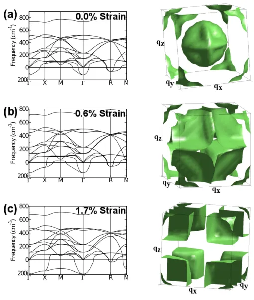
octahedra, and the unstable polar mode at Γ. An alternative way to visual-ize the distribution of lattice instabilities in reciprocal space is by plotting the
ω2 = 0 isosurface in the first Brillouin zone [175, 63], Fig. 2.2(b). The enclosed
volumes on the zone boundary correspond to the R-point octahedral rotation instability and the FE instability is associated with the volume in the zone cen-ter. We point out that this picture is similar to that obtained by Lasotaet al.,[97] who previously considered the coherence properties of theR-point rotation in-stability only. Fig. 2.2(a) shows that the branch stemming from theΓinstability becomes stable at wave vectors away fromΓin all the of high symmetry direc-tions – towards X, M or R – and is therefore localized in reciprocal space to a finite volume around the zone center.
From Fig. 2.2(b) it is seen that the volume of the FE instability has a strongly anisotropic structure: it consists of three perpendicular disks. Each disk en-closes wave vectors that have an instability involving ionic displacements in the direction perpendicular to the plane of the disk. The finite thickness of the disks, corresponding to a finite longitudinal coherence length,l|| ∼ 1/q||, has been pre-viously discussed in perovskite ferroelectrics such as BaTiO3 [63] and KNbO3
[175]. The finite radius of the unstable disks in the reciprocal space found in SrTiO3 suggests that the frequency of the unstable branch also depends on the
perpendicular component of the wavevector, corresponding to a finite perpen-dicular coherence length,l⊥∼1/q⊥(See Section 2.8.1). In contrast, in BaTiO3[63]
and KNbO3[175] the isosurfaces consist of three almost perfectly flat slabs that
are infinitely extended, indicating that the frequency of the unstable branch is the same regardless of the component of the wavevector that is perpendicular to the direction of the ionic displacements. This implies that the critical thickness for an infinite slab of BaTiO3is zero [59].
different perovskite blocks (we will shortly prove this is true), the non-vanishing critical thickness required for ferroelectricity in SrTiO3imposes a geometric
con-dition,ncrit, for RPs to display an in-plane ferroelectric instability;n< ncrit
mem-bers cannot have an energy lowering FE distortion simply because the number of perovskite blocks between the rocksalt layers do not satisfy the coherence condition. However, as n increases, the structures should get closer to the FE transition. This is exactly what we have shown in Fig. 2.1, where the soft mode frequencyωvanishes atncrit ∼ 7, agreeing with the lower bound from the
recip-rocal space picture of the instability of SrTiO3.
2.5
Tuning the Coherence Length
The effects of strain [43] and pressure [146] on ferroelectricity in perovskites are well known; they alter the balance between the short-range forces (which favor the centrosymmetric state) and long-range Coulomb forces (which favor the fer-roelectric state). But what are their effects on the coherence requirements? In Fig. 2.2 (b) and (c) we plot the phonon dispersion curves and the corresponding ω2 = 0isosurfaces of cubic SrTiO
3for isotropic tensile strains of 0.6% and 1.7%,
respectively. As shown, negative pressure not only softens theΓinstability (the well-known strain-induced ferroelectricity [8]) but also increases the volume of unstable q-vectors in reciprocal space. By 0.6% strain, the instability reaches the X point and at 1.7% strain the branch is unstable and relatively dispersionless in the entireΓ-X-M plane. In fact, theω2 = 0isosurface at this isotropic strain
value resembles that of BaTiO3 [63]. We presentω2 = 0 isosurfaces for SrTiO3
under tensile biaxial strain in Fig. 2.3. The tensile biaxial strain boundary con-dition results in two components of the polar mode soften whereas the third
Γ X M Γ R M 200i 0 200 400 600 800 Fr eq ue nc y (c m -1 ) Γ X M Γ R M 200i 0 200 400 600 800 Fr eq ue nc y (c m -1 ) Γ X M Γ R M 200i 0 200 400 600 800 Fr eq ue nc y (c m -1 ) qz qx
(a)
Figure 2.2: Phonon dispersions of SrTiO3 in its cubic (Pm¯3m) phase at
(a) experimental volume, and under (b) 0.6 % and (c) 1.7 % isotropic tensile strain with respect to the experimental lattice constant. The correspondingω2 = 0isosurfaces are shown next
(out-of-plane) component hardens. This results in two of the three disks in the reciprocal space getting larger, while the third one shrinks.
These results suggest that under increasing biaxial, in-plane tensile strain [147] the critical thickness for in-plane ferroelectricity in SrTiO3, and
hence ncrit in the RPs, should decrease and eventually vanish. This is clearly
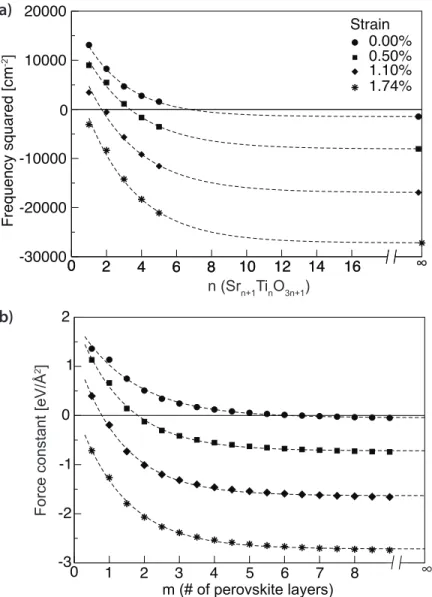
seen for the RPs in Fig. 2.4(a). Note that at a tensile strain value of 1.1% – a strain more than sufficient to drive SrTiO3ferroelectric – the perpendicular coherence
length (l⊥) in SrTiO3is still non-zero. This results in then=1RP remaining very
far from displaying a polar instability. It isn’t until a strain of∼1.4% thatl⊥ ≈ 0 and then=1structure develops a polar instability.
As further proof of a crossover from 2d to 3d ferroelectric behavior (and the direct strain control thereof), we parameterize from first-principles a finite thick, infinite perovskite slab force constant model for which we add additional layers of SrO and TiO2planes. (For details, see Section 2.8.2.) The softest force constant
eigenvalue is plotted in Fig. 2.4b for different strain values as the number of SrTiO3 layers, m, is increased. Notice that the in-plane polar force constant in
this 2d model slab (Fig. 2.4b) is evolving with both thickness and strain exactly like the in-plane polar instabilities in the structurally 3d RPs (Fig. 2.4a). This is clear evidence of the proposed coherence physics and the direct control of with strain. (A similar calculation for unstrained BaTiO3, which has al⊥ ≈ 0, shows that a single TiO2layer in bulk BaTiO3is unstable.)
qx q y qx q y qx q y qx qy
(a)
(b)
(c)
(d)
Figure 2.3: Theω2 = 0 isosurfaces for SrTiO
3 under (a) 0.0%, (b) 0.5%, (c)
1.1%, and (d) 1.7% biaxial strain. Right panels show the cuts of the isosurfaces onkz = 0 planes. For (c) and (d), the slight anisotropy on the surfaces of DyScO3 and GdScO3 substrates
are taken into account, however, this anisotropy gives barely visible results.
m (# of perovskite layers)
∞
Force constant [eV/Å
2] a) b) 0 10 12 14 16 -30000 -20000 -10000 0 10000 20000 Frequency squared [cm -2] 2 4 6 8 n (Srn+1TinO3n+1) 0.00% 0.50% 1.10% 1.74% Strain -2 -1 0 1 2 ∞ 0 2 4 6 8 10 12 14 16 ∞ 0 1 2 3 4 -3 5 6 7 8
Figure 2.4: (a) Ruddlesden-Popper, (SrTiO3)n(SrO): In-plane polar soft
mode frequency squared versus layering number n. (b) Per-ovskite Slab Model, (SrTiO3)m: Lowest in-plane polar
inter-planar force constant matrix eigenvalue versus thickness of SrTiO3. Strain values are given with respect to the lattice
con-stant of SrTiO3. The slab thickness in panel b, given in number
of SrTiO3layers, corresponds to half the number of atomic SrO
or TiO2 layers in the slab. Half integer values correspond to
an odd number of atomic layers that are terminated by TiO2
layers o both sides. Similar calculations for slabs terminated by SrO layers, not presented here, give qualitatively similar re-sults even though the force constants are higher for small thick-nesses. The lines are fits to exponentials.
2.6
The Effect of Rumpling
These results suggest that the rocksalt layer in Srn+1TinO3n+1 breaks the
coher-ence between perovskite blocks. Why and how? Note that rumpling of the SrO layers is permitted by symmetry in paraelectric RPs and that the distance along the[001]direction between the Sr and O ions within the rocksalt layer can be as large as 0.20 Å [51] and quickly gets smaller in the layers further away, Fig. 2.5(b). In RPs with n > ncrit, the in-plane polar displacements of Ti along
the infinite Ti-O-Ti chains get smaller the closer the chain is to the rocksalt layer. We propose that the rumpling at the double SrO layers breaks the coherence between perovskite slabs.
To test this hypothesis, we artificially zero the rumpling by moving the Sr and Ti atoms to exactly the same plane as the oxygens, and repeat the phonon calculations. We find that even then = 1 Sr2TiO4 under zero strain has an
in-plane polar instability and it is in fact almost equal in magnitude to that of SrTiO3, that is, the decay of the phonon frequency withndisappears1.
2.7
A Novel Polar State
What are the implications of our findings? We propose that strained RPs, which lack coherence across the rocksalt layers, can not be ferroelectric, but rather dis-play a novel polar state. In Fig. 2.5c we plot the energy versus mode amplitude in, e.g., Sr4Ti3O7 (n = 3) for both the ferroelectric mode and an antiferroelectric
distortion involving polar distortions of neighboring perovskite slabs
antipar-1Note that strain has little influence on the amount of rumpling; rumpling does not differ by
allel to each other (Fig. 2.5a shows a comparison of these modes). Notice that the energy surfaces for these distortions are degenerate up to the precision of this plot. In Fig. 2.5d we plot the results of a similar calculation except that the rumpling was artificially zeroed; without rumpling, the degeneracy of the AFE and FE modes is lifted. These calculations (we found similar results for n= 1, 2 and 3 at two different values of strain) prove that the RP fault indeed breaks the coherence between perovskite slabs, resulting not only in a suppression of polar distortions forn< ncrit, but also forn>ncritpolar distortions in neigboring
perovskite slabs do not interact with each other significantly even at higher than quadratic order. All of this suggests that there are an infinite number of degen-erate states involving uncorrelated atomic-scale polar regions. We surmise that the ground state may be a form of relaxor ferroelectricity without disorder, the consequences of which remain unclear.
2.8
Auxiliary Material
In this section, we provide some details of the arguments and calculations that are used in preceding sections. In Section 2.8.1, we explain how to obtain a crude estimate of the critical thickness from bulk phonon dispersions. In Section 2.8.2, we explain the details of the toy model that makes use of the Interplanar Force Constants. Finally, in Section 2.8.3, we calculate the energy gain with respect to the paraelectric state in the polar state and estimate the criticalnthat a polar distortion can experimentally be observed in.
Mode Amplitude (Arbitrary Units) -10
-5 0 5
Energy Gain (meV/f.u.)
AFE FE With Rumpling Antiferroelectric Ferroelectric a) }0.232 Å }0.041 Å }0.036 Å b)
Mode Amplitude (Arbitrary Units) -10
-20 20 10 0
Energy Gain (meV/f.u.)
AFE FE
Without Rumpling
c) d)
Figure 2.5: Sr4Ti3O10 ground state under 1.1%tensile strain. (a) Schematic
of ferroelectric (FE) and antiferroelectric (AFE) distortions. (b) Rumpling distortion (defined as the distance along [001] be-tween cations and oxygens on the same layer). (c) Energy gain due to FE and AFE distortions in structures with rumpling. (d) The same as (c) except the rumpling distortion has been artifi-cially set to zero.
2.8.1
Perpendicular Coherence Length
It is possible to obtain information about the perpendicular coherence proper-ties of a ferroelectric instability from the phonon dispersions of the high symme-try (paraelectric) structure. Let us consider a cubic structure withxˆ,yˆandˆzaxes aligned with the (100) directions, and focus on thezˆcomponent of polarization only. Fig. 2.6 includes the sketch of distortion patterns corresponding to
vari-ous wave vectors withqz = 0. The argument for BaTiO3 [1] or KNbO3 [2] is the
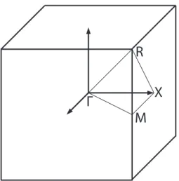
following: As the unstable branch is dispersionless in the wholeΓ- X - M plane, all of the distortion patterns in Fig. 2.6 are equally unstable. (See Fig. 2.7 for the labels of high symmetry points.) This indicates that whether a mode on the polar branch is unstable or not does not depend on the variation of displace-ment pattern in the direction perpendicular to the polarization, and so a one unit cell thick chain of atoms is unstable by itself – even if all the atoms in the rest of the crystal are fixed in their high symmetry positions. (One can imagine taking a superposition of phonon modes with different wave vectors to obtain a distortion pattern where only ions on such a thin chain are displaced.) Hence, the perpendicular coherence lengths for BaTiO3 and KNbO3 are zero. In other
words, in a BaTiO3 or KNbO3 crystal in its high symmetry paraelectric phase,
a coherent displacement of atoms that form a single unit cell thick chain can reduce energy.
The situation is different for (unstrained) SrTiO3. Referring to Fig. 2.2a,
while there is a Γ point instability with local polar atomic displacements as shown in Fig. 2.6(a), the branch stemming from this instability is stable at the X (Fig. 2.6(c)) and M (Fig. 2.6(e)) points. Therefore the polar instability is lo-calized around the Γ-point in the q-space, stiffening as one transverses about halfway alongΓ- X (Fig. 2.6(b)) and also alongΓ - M (Fig. 2.6(d)) points. This indicates that the frequency of the polar branch isnot independent of the per-pendicular component of the wave vector. A superposition of modes over this restricted volume of unstable phonon modes results in a finite thickness of the Ti-O-Ti chains. The minimum thickness of this unstable distortion is inversely proportional to the radius of the disks in figure 2a of main text (q⊥in Fig. 2.8), as this radius sets the number of unstable phonon modes that can be superposed