Modelling bonds and credit default swaps using a
structural model with contagion
Haworth, Helen; Reisinger, Christoph; Shaw, William
Postprint / Postprint
Zeitschriftenartikel / journal article
Zur Verfügung gestellt in Kooperation mit / provided in cooperation with:
www.peerproject.eu
Empfohlene Zitierung / Suggested Citation:
Haworth, H., Reisinger, C., & Shaw, W. (2008). Modelling bonds and credit default swaps using a structural model with contagion. Quantitative Finance, 8(7), 669-680. https://doi.org/10.1080/14697680701834614
Nutzungsbedingungen:
Dieser Text wird unter dem "PEER Licence Agreement zur Verfügung" gestellt. Nähere Auskünfte zum PEER-Projekt finden Sie hier: http://www.peerproject.eu Gewährt wird ein nicht exklusives, nicht übertragbares, persönliches und beschränktes Recht auf Nutzung dieses Dokuments. Dieses Dokument ist ausschließlich für den persönlichen, nicht-kommerziellen Gebrauch bestimmt. Auf sämtlichen Kopien dieses Dokuments müssen alle Urheberrechtshinweise und sonstigen Hinweise auf gesetzlichen Schutz beibehalten werden. Sie dürfen dieses Dokument nicht in irgendeiner Weise abändern, noch dürfen Sie dieses Dokument für öffentliche oder kommerzielle Zwecke vervielfältigen, öffentlich ausstellen, aufführen, vertreiben oder anderweitig nutzen.
Mit der Verwendung dieses Dokuments erkennen Sie die Nutzungsbedingungen an.
Terms of use:
This document is made available under the "PEER Licence Agreement ". For more Information regarding the PEER-project see: http://www.peerproject.eu This document is solely intended for your personal, non-commercial use.All of the copies of this documents must retain all copyright information and other information regarding legal protection. You are not allowed to alter this document in any way, to copy it for public or commercial purposes, to exhibit the document in public, to perform, distribute or otherwise use the document in public.
By using this particular document, you accept the above-stated conditions of use.
For Peer Review Only
Modelling Bonds & Credit Default Swaps using a Structural Model with Contagion
Journal: Quantitative Finance
Manuscript ID: RQUF-2006-0113.R1
Manuscript Category: Research Paper
Date Submitted by the
Author: 26-Jun-2007
Complete List of Authors: Haworth, Helen; University of Oxford, OCIAM Reisinger, Christoph; University of Oxford, OCIAM Shaw, William; King's College London, Mathematics
Keywords: Contagion, Correlation Modelling, Credit Models, Credit Default Swaps, Credit Risk, Defaultable Securities
JEL Code:
C0 - General < C - Mathematical and Quantitative Methods, G13 - Contingent Pricing|Futures Pricing < G1 - General Financial Markets < G - Financial Economics, G33 - Bankruptcy|Liquidation < G3 - Corporate Finance and Governance < G - Financial Economics
Note: The following files were submitted by the author for peer review, but cannot be converted to PDF. You must view these files (e.g. movies) online.
For Peer Review Only
Modelling Bonds & Credit Default Swaps using a Structural
Model with Contagion
Helen Haworth∗, Christoph Reisinger∗ and William Shaw†
Revised version, June 2007
Abstract
This paper develops a two-dimensional structural framework for valuing credit default swaps and corporate bonds in the presence of default contagion. Modelling the values of related firms as correlated geometric Brownian motions with exponential default barriers, analytical formulae are obtained for both credit default swap spreads and corporate bond yields. The credit dependence structure is influenced by both a longer-term correlation structure as well as by the possibility of default contagion. In this way, the model is able to generate a diverse range of shapes for the term structure of credit spreads using realistic values for input parameters.
1
Introduction
Firms do not operate in isolation and company defaults are not independent. In reality a whole network of links exists between companies in related businesses, industries and markets and the impact of individual credit events can ripple through the market as a form of contagion. It is thus of fundamental importance when modelling credit, not only to understand the drivers of credit risk at an individual company, but also the dependence structure between related companies. Whether accounting for counterparty risk in the price of a single-name credit derivative, or considering credit risk in a portfolio context, an understanding of credit dependence is essential to accurate risk evaluation and pricing.
Credit weakness, ratings downgrades and ultimately corporate default can occur in three main ways. Firstly, a company may be adversely affected for reasons specific to that company alone (e.g. poor financial management). Secondly, credit weakness may occur due to a factor or factors impacting multiple companies – whether in the form of a cyclical influence related to the economy, or a market-wide shock such as an earthquake or September 11th. Finally, ∗The Nomura Centre for Mathematical Finance, OCIAM Mathematical Institute, Oxford University, 24-29
St Giles, Oxford, OX1 3LB, England. email: [email protected]. This work is kindly supported by Nomura and the EPSRC. We are grateful to Sam Howison and Ben Hambly for helpful input and discussions.
†King’s College, The Strand, London, WC2R 2LS, England
5 6 7 8 9 10 11 12 13 14 15 16 17 18 19 20 21 22 23 24 25 26 27 28 29 30 31 32 33 34 35 36 37 38 39 40 41 42 43 44 45 46 47 48 49 50 51 52 53 54 55 56 57 58 59 60
For Peer Review Only
companies are related through ties, some of which are real (e.g. a trade-creditor agreement), others of which are purely a matter of perception – for example the fear of accounting fraud. Credit dependence then occurs primarily through two mechanisms – either as a direct conse-quence of a common driving factor, or due to inter-company ties. The latter can be thought of as a form of contagion.
The purpose of this paper is to examine the importance of considering a more complete de-pendence structure than is usually incorporated in credit models, one that better reflects reality, taking into account both a common driving influence and the possibility of idiosyn-cratic company links. To do so, whilst retaining some degree of analytical tractability, we consider a two-dimensional structural model with default as the first hitting time of an ex-ponential barrier. Firm values are modelled as correlated geometric Brownian motions and the default event is contagious. In this way, we are able to capture the two facets of the dependence structure. The correlation in firm values reflects a longer-term common driving influence on corporate strength whilst default contagion represents a direct link between the fortunes of both companies. As discussed in Section 3, this framework results in a model that is asymmetric with regard to default risk, a significant improvement on prior models.
Structural models, whilst far from straightforward mathematically, are far more grounded in economic fundamentals than many other models and thus form a good starting point for a realistic description of credit dynamics. Giesecke (2004), Sch¨onbucher (2003) and Lando (2004) provide a good introduction to structural models, their development since first intro-duced by Merton (1974), and their traditional place within credit modelling. Until recently, the vast majority of work on the structural model has focused on the case of a single firm. In-deed, two popular commercial packages, Moody’s KMV and CreditGradesT M, are motivated by the single-firm structural model1. Very little, however, has been published for multiple
companies, with the market mainly focused on copulas or conditionally independent factor models2 in the multivariate case. Two exceptions are the papers by Zhou (2001) and Hull and White (2001). Zhou (2001) calculates default correlations for two firms whose asset values are modelled as correlated Brownian motions. Hull and White (2001) extend this to framework to higher dimensions and proceed numerically in a discrete-time setting, proposing a method to calibrate piecewise constant default barriers to a term structure of default hazard rates. In contrast, we extend the framework used in Zhou (2001) to incorporate default contagion and derive analytical formulae for bond yields and CDS spreads.
Copula methods, which allow the dependence structure of a portfolio to be considered inde-pendently from individual default times, are easy to implement and have rapidly become the market standard for modelling portfolios of credits. However, as basically static models able only to model expected defaults over a given time period, they fail to allow for suitable credit spread dynamics and tend to exhibit time instabilities.3 Furthermore, the copula approach has no notion of default cause and effect as exists in a contagion mechanism.
As problems have arisen with the widespread market use of copulas, multidimensional
struc-1Further details of these approaches can be found at www.moodyskmv.com and in Finger et al. (2002),
respectively.
2For a good overview of the use of copulas in finance, see Cherubini et al. (2004); Sch¨onbucher (2003)
provides a useful summary and references for factor models.
3Mikosch (2006) provides a critical discussion of the widespread usage of copula methods; some countering
arguments are given by Genest and Remillard (2006). 6 7 8 9 10 11 12 13 14 15 16 17 18 19 20 21 22 23 24 25 26 27 28 29 30 31 32 33 34 35 36 37 38 39 40 41 42 43 44 45 46 47 48 49 50 51 52 53 54 55 56 57 58 59 60
For Peer Review Only
tural models are seeing renewed interest. Hull et al. (2005) price CDO tranches in a structural framework where assets are driven by a common factor. In this way, defaults are modelled in a dynamic setting, and firm value correlations can be time-dependent or stochastic, however the dependence structure stems purely from the correlated firm values and so is unable to account for any default causality or contagion. In another approach, Luciano and Schoutens (2005), Moosbrucker (2006) and Baxter (2006) assume that firm values are driven by Levy processes rather than geometric Brownian motions. By assuming that firm values are mod-elled as geometric Brownian motions time-changed by a common Gamma business time, firm values become Variance Gamma processes, allowing for a richer characterisation of spread dy-namics. Dependence is introduced through having a common stochastic time change, which may then be further broken down into systematic and idiosyncratic components, with a num-ber of different representations proposed by the various authors. The resultant dependence structure is more realistic and flexible but does not incorporate any form of default contagion. The paper is organised as follows. In Section 2 we outline the framework for the model, its assumptions and underlying results. We consider both the most general formulation and cases in which the formulae simplify. Formulae and results for corporate bond yields are provided in Section 3, whilst those for credit default swap spreads are in Section 4. We summarise and consider future extensions in Section 5. Mathematical details are in the appendix.
2
The Model
We consider two companies, firm values Vi, i = 1,2. Each company issues equity and a
single homogeneous class of debt, assumed to be a zero coupon bond,Ci(t, T), par value Ki,
maturityT. For simplicity we assume that both bonds have the same maturity date but the analysis is easily extendible to different maturity dates.
For each company, firm value is assumed to follow a geometric Brownian motion, with default as the first time that the value of the firm hits a lower default barrier bi(t). As in Merton
(1974) and Black and Cox (1976), we assume that a firm’s value can be constructed from tradable securities and so in the risk-neutral pricing measure, fori= 1,2,
dVi(t) = (rf −qi)Vidt+σiVidWi(t)
where the risk-free rate, rf, dividend yields,qi, and volatilities, σi, are constants, Wi(t) are
Brownian motions and cov(W1(t), W2(t)) =ρt for constant correlationρ.
We assume that each company has an exponential default barrier, reflecting the existence of debt covenants, and denote the default barrier for companyiby
bi(t) =Kie−γi(T−t).
Whilst similar to the barrier formulation in Black and Cox (1976)4, defining the barrier in this way provides us with additional flexibility, enabling us to change its slope. In particular, in the special case that the barrier growth rate is set equal to the drift in firm value, the model simplifies. As neither the barrier growth rate nor the drift in firm value is observable
4Black and Cox (1976) use a barrier of the formω
iKie−rf(T−t) where 0 ≤ωi ≤ 1. The similarities and
differences in this formulation compared to the one we use are discussed further in Section 3. 5 6 7 8 9 10 11 12 13 14 15 16 17 18 19 20 21 22 23 24 25 26 27 28 29 30 31 32 33 34 35 36 37 38 39 40 41 42 43 44 45 46 47 48 49 50 51 52 53 54 55 56 57 58 59 60
For Peer Review Only
in practice, this is an attractive simplification. It is by no means necessary for our analysis, however, and we provide results for the most general case.
Setting Xi(t) = ln Vi(t) Vi(0) e−γit
enables us to consider the simpler case of Brownian motion with drift and constant default barrierBi= ln bi(0) Vi(0) ≤0. Xi(0) = 0 and Xi(t) =αit+σiWi(t) whereαi =rf −qi−γi−12σ2i.
Defining the running minimum
Xi(t) = min
0≤s≤tXi(s),
and default time, τi, as the first hitting time of the default barrier, τi= inf{t:Xi(t) =Bi},
survival probability is then
P(τi > s) =P(Xi(s)≥Bi).
The key result we use to value credit spreads is the joint survival probability density function and the resultant joint survival probability,P(t),
P(t) = P(X1(t)≥B1, X2(t)≥B2) (1) = 2 βte a1B1+a2B2+bt ∞ X n=1 e−r20/2tsin nπθ0 β Z β 0 sin nπθ β gn(θ) dθ where gn(θ) = Z ∞ 0 re−r2/2teA(θ)rI(nπ β ) rr0 t dr a1 = α1σ2−ρα2σ1 (1−ρ2)σ2 1σ2 , a2= α2σ1−ρα1σ2 (1−ρ2)σ 1σ22 b = −α1a1−α2a2+ 1 2σ 2 1a21+ρσ1σ2a1a2+ 1 2σ 2 2a22 tanβ = − p 1−ρ2 ρ , β∈[0, π] r0 = 1 p 1−ρ2 B12 σ2 1 − 2ρB1B2 σ1σ2 +B 2 2 σ2 2 1/2 tanθ0 = σ1B2 p 1−ρ2 σ2B1−ρσ1B2 , θ0∈[0, β] A(θ) = a1σ1sin(β−θ) +a2σ2sinθ, 6 7 8 9 10 11 12 13 14 15 16 17 18 19 20 21 22 23 24 25 26 27 28 29 30 31 32 33 34 35 36 37 38 39 40 41 42 43 44 45 46 47 48 49 50 51 52 53 54 55 56 57 58 59 60
For Peer Review Only
and I(nπ β ) rr0 tis a modified Bessel’s function. P(t) represents the probability that neither company hits its default barrier by time t. Correlation between firm values is reflected by β, with β = π corresponding to perfect correlation, β =π/2 independence and β = 0 perfect negative correlation. When the drifts in firm value and the default barrier are equal,αi = 0,
leading to ai = 0 = b. The form of P(t) derives from the separation of variables in the
solution of the Fokker-Planck equation governing the evolution of the survival probability density function. Full details of the calculation methodology can be found in the paper by Hua et al. (1998) in which double lookbacks are valued using the joint distributions for the maxima and minima of two correlated Brownian motions. Zhou (2001) uses the same result to calculate default correlation for two companies with correlated assets. In particular, Zhou5 primarily considers the special case that the barrier growth rate and drift in firm value are equal,γi=rf −qi−12σ2i, and shows that
P(t) =√2r0 2πte −r2 0/4t X n=1,3,... 1 nsin nπθ0 β I12( nπ β +1) r20 4t +I1 2( nπ β −1) r20 4t . (2)
This simplification, implying constant leverage, makes the joint survival probability consid-erably faster to evaluate. Zhou (2001) found that the assumption had minimal impact on default correlations for shorter maturities. Supporting this finding we see very little difference in survival probabilities as the barrier growth rate, γi, is changed for maturities up to five
years. This is reflected in the fact that implied bond yields are not very sensitive to changes in the barrier growth rate, as illustrated in Figure 4.6
The joint survival probability calculation can also be simplified by selecting values of β for which the modified Bessel’s function simplifies – for example β = πk for integer k. Unfor-tunately, since ρ = −cosβ, the majority of these cases correspond to negative values of correlation and so are of only limited interest in our framework.
3
Bond Yield Calculation
The value of a corporate bond to a bondholder arises from two components – its value on maturity (should it mature) and its value in the event of default. We consider thet= 0 value of a zero coupon bond issued by company one, par valueK1, maturing at time T, denoted C1(0, T). The yield is then
y1(0, T) =− 1 T ln C1(0, T) K1 . (3)
We incorporate default contagion by assuming that company one defaults on its outstanding debt the first time that the value of either company reaches its default barrier. In this
5N.B. The definitions ofa
1anda2 in Zhou are the negative of the definitions in this paper. Our formula for
gn(θ) can be reconciled with Zhou’s using double angle formulae and the fact that cosβ=−ρ, sinβ= p
1−ρ2.
(His angleαis our angleβ.)
6An extensive analysis of survival probability sensitivity to input parameters is contained in Haworth (2006);
here we consider solely the impact of key parameter assumptions with regard to credit spreads, with results in Section 3. 5 6 7 8 9 10 11 12 13 14 15 16 17 18 19 20 21 22 23 24 25 26 27 28 29 30 31 32 33 34 35 36 37 38 39 40 41 42 43 44 45 46 47 48 49 50 51 52 53 54 55 56 57 58 59 60
For Peer Review Only
way, there are two components to the default mechanism. If the value of firm one declines sufficiently, the company is forced into bankruptcy – this is due to the direct performance of the company itself and is exactly the framework used in normal first-passage structural models. The second way in which company one can default is if company two goes bankrupt, modelled as the time when the value of company two reaches its default barrier – default contagion. This would be the situation if company two was essential to the continuing operation of company one. For example if company two was the only purchaser of company one’s products, as in the case of a small or regional auto-parts supplier to General Motors.
Our specification of the contagion mechanism implicitly assumes that the full extent of its existence is not known to the market beforehand,7 as is so often the case. Many links between companies are very opaque and certainly not fully disclosed. For example, the full nature of a bank’s loan portfolio is rarely apparent, and there are many instances when banks have ended up over-exposed to one company or industry. The situations at Parmalat and LTCM in recent years are cases in point. Another example is the networks of business links that exist, for example in Italy, when extensive corporate cross-holdings are common. Few of these are publicly known. Too frequently, the existence or full extent of a company’s relationships and the consequent investment risks only come to light when problems arise. The goal of our model is to take the first step in considering the spread implication of these types of links through the introduction of a contagion process that is simple enough to allow for analytical solutions. It is worth noting that company two need not default automatically if company one does. It can continue to operate regardless of the financial viability of company one with dependence solely through the asset correlation,ρ. As a result, the model is asymmetric with respect to default risk, in stark contrast with the majority of previous models incorporating a credit dependence structure.8
This framework is only really realistic for ρ≥0. It is highly unlikely that the bankruptcy of one company would lead to the immediate default of another, negatively correlated company. Whilst it is possible to contrive a theoretical example (e.g. a highly diversified company like General Electric might be key to one of its suppliers, but negatively correlated with it overall), economically it is rather improbable in practice and so we restrict ourselves to consideration of 0≤ρ≤1.
Similarly to Black and Cox (1976), we assume that
Payment at maturity = min(ω1V1(T), K1) provided τ1 > T, τ2> T
whereK1 is the par value of the bond, τi denotes the default time of companyi, and ω1 is a
constant write down factor. This factor is the same as used later in the specification of the payment on default. It represents the fact that in the event of default or a restructuring, a portion of the defaulting company’s value is lost to bondholders. This is commonly seen in practice, caused, for example, by restructuring costs or violation of the priority rule allocating claims in the event of default.
7We are grateful to one of our referees for highlighting this.
8The natural extension of this framework to larger portfolios of companies would be the type of situation
considered in Jarrow and Yu (2001) in which ‘primary’ companies impact ‘secondary’ companies but not vice versa. A ‘primary’ company is likely to be larger with a greater market impact than a ‘secondary’ company. For example Microsoft or General Motors compared to a small, local IT or auto component manufacturer. 6 7 8 9 10 11 12 13 14 15 16 17 18 19 20 21 22 23 24 25 26 27 28 29 30 31 32 33 34 35 36 37 38 39 40 41 42 43 44 45 46 47 48 49 50 51 52 53 54 55 56 57 58 59 60
For Peer Review Only
Black and Cox (1976) incorporate the write-down factor in the default barrier, but then the bondholders are always paid in full once the value of the firm at maturity is at least the face value of the bonds. This seems a little unrealistic since a company would be unable to pay out its entire value to bondholders. There would be liquidation costs and a company would not be able to raise its entire value in a refinancing. It therefore makes sense that the firm value at maturity must be equal to someK1/η1, whereω1 ≤ η1 ≤ 1, for bondholders to be
fully repaid. For simplicity, since fewer parameters are preferable, we assume that the firm repays bondholders in full for V1(T) ≥ K1/ω1. This would seem to be an improvement on
the case where full repayment occurs for firm value at maturity of par or more.
Changing toXi(t) coordinates, the discounted maturity payment, DMP, can be written
DMP = e−rfT Z ∞ B2 Z ∞ d K1p(x1, x2, T) dx1dx2 +e−rfT Z ∞ B2 Z d B1 ω1V1(0)ex1+γ1Tp(x1, x2, T) dx1dx2 where p(x1, x2, T) = ∂2 ∂x1∂x2P (X1(T)≤x1, X2(T)≤x2, X1(T)≥B1, X2(T)≥B2) (4)
is the joint survival probability density function at maturity and
d= ln K1
ω1V1(0)−
γ1T =B1−lnω1 ≥B1.
As outlined in Appendix A, integrating and making a change of variables, DMP = H1(T) ∞ X n=1 sin nπθ0 β Z β 0 sin nπθ β g+n(θ) dθ (5) +H2(T) ∞ X n=1 sin nπθ0 β Z β 0 sin nπθ β g∗n(θ) dθ where H1(T) = 2K1e−rfT βT e a1B1+a2B2+bTe−r20/2T H2(T) = 2ω1V1(0)e(γ1−rf)T βT e (a1+1)B1+a2B2+bTe−r02/2T gn+(θ) = Z ∞ d∗(θ) re−r2/2TeA(θ)rI(nπ β ) rr0 T dr gn∗(θ) = Z d∗(θ) 0 re−r2/2Te[A(θ)+σ1sin(β−θ)]rI (nπβ ) rr0 T dr d∗(θ) = d−B1 σ1 hp 1−ρ2cosθ+ρsinθi = lnω1 σ1sin(θ−β) ≥ 0. 5 6 7 8 9 10 11 12 13 14 15 16 17 18 19 20 21 22 23 24 25 26 27 28 29 30 31 32 33 34 35 36 37 38 39 40 41 42 43 44 45 46 47 48 49 50 51 52 53 54 55 56 57 58 59 60
For Peer Review Only
We assume that default occurs the first time that either company hits its default barrier and that in the event of default, the bondholder receives a percentage of discounted par value,ω1K1e−rf(T−τ). This is the same payoff as used by Black and Cox (1976) and is highly
attractive since the discounted default payment then becomes
ω1K1e−rfT(1−P(T)), (6)
where the joint survival probability P(T) =P(X1(T)≥B1, X2(T)≥B2) is defined in (1).
By construction, the default payment is worth less than discounted par, and so for consistency we just need to ensure that it is worth less than the value of the firm at default. Since company one must be worth at least as much as its default barrier, a sufficient condition is
ω1 ≤e(rf−γ1)(T−τ1).
Adding together (5) and (6), and using (1) forP(T), yields can then be calculated using (3). In order to evaluate (5) and (6) we use the integral form of the modified Bessel’s function,
I(nπ β ) rr 0 t = 1 π Z π 0 errt0cosφcos nπφ β dφ− 1 πsin nπ2 β Z ∞ 0 e− rr0 t coshs− nπs β ds.
The infinite sums in (5) and (6) converge rapidly to zero, and so this substitution enables us to approximate solutions by a finite sum of three-dimensional integrals which we evaluate by numerical quadrature using a sparse grid (for further information regarding sparse grid methods, see Gerstner and Griebel (1998)). Figures 1 - 6 illustrate results and parameter sensitivities. As a measure of company strength we consider initial firm value,Vi(0), divided
by the initial level of the barrier, bi(0). We denote this parameter by initial credit quality
and spread sensitivity to it is as would be expected – as initial credit quality declines, spreads widen significantly. An indicative scaled distance to default, σ1
ilog(
Vi(0)
bi(0)), for our parameter values ofσi = 0.2 and initial credit quality of 2 is then 3.5.
In all cases, we see that yields decline as correlation increases. Since default is less likely with increasing correlation,9 the bond is less risky, bond-holders are not rewarded with such high returns, increasing the price and reducing the yield.
Figures 1 and 2 illustrate the yield curve for two values of the write-down factor,ω1.
Compar-ing them, we see that asω1 decreases, the yield curve inverts. The extent to which payments
are written down clearly has a large impact on yields, particularly at the short-end of the yield curve. The thick black line, labelled ‘none’ in the figures is the bond yield for a firm with the same parameter values, but operating in isolation. In other words, a single firm’s yield when modelled in a first-passage framework, but with no exposure to another company through default contagion. As one would expect, yields are lower as such a firm’s bonds are less risky. It is immediately apparent that allowing for default contagion has a significant impact on yields, especially for longer-dated bonds.
Figure 3 shows the impact of varyingω1 on a five-year bond. Of note, the case when ω1 = 1
corresponds to no write-down on default and in effect the bond becomes risk-free, yielding,
9This is the case whether or not there is default contagion and can be seen from the fact that the probability
of at least one of the companies defaulting in a given time period decreases as they become more correlated. IfNidenotes default by companyi, fori= 1,2, thenP(N1∪N2) =P(N1) +P(N2)−P(N1∩N2) and the final
term increases withρ. 6 7 8 9 10 11 12 13 14 15 16 17 18 19 20 21 22 23 24 25 26 27 28 29 30 31 32 33 34 35 36 37 38 39 40 41 42 43 44 45 46 47 48 49 50 51 52 53 54 55 56 57 58 59 60
For Peer Review Only
Figure 1: Implied yield curve,ω1 = 0.7
1 2 3 4 5 6 7 8 9 10 5.2 5.4 5.6 5.8 6 6.2 6.4 6.6 6.8 7 Time ρ = 0 ρ = 0.4 ρ = 0.7 ρ = 0.9 None
Figure 2: Implied yield curve,ω1 = 0.5
1 2 3 4 5 6 7 8 9 10 6 7 8 9 10 11 12 13 Time ρ = 0 ρ = 0.4 ρ = 0.7 ρ = 0.9 None σ1=σ2= 0.2, K1= 100, rf = 0.05,
q1=q2= 0, γ1=γ2= 0.03, initial credit quality = 2
as we would expect, the risk-free rate of 5% regardless of correlation. ω1 acts in two ways –
it lowers the payment in the event of default and it increases the value the company must be worth at maturity for bondholders to be repaid in full.
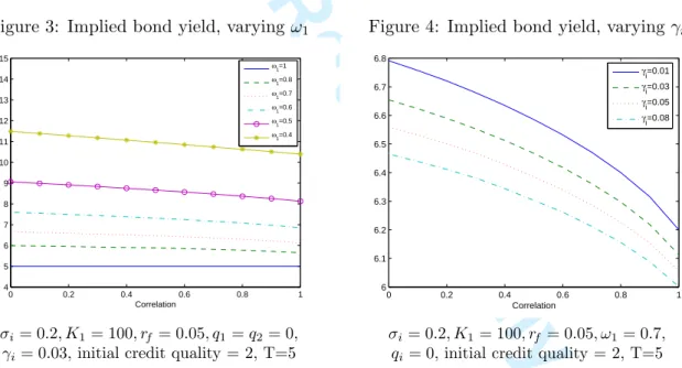
Figure 3: Implied bond yield, varyingω1
0 0.2 0.4 0.6 0.8 1 4 5 6 7 8 9 10 11 12 13 14 15 Correlation ω1=1 ω1=0.8 ω1=0.7 ω1=0.6 ω1=0.5 ω1=0.4 σi = 0.2, K1= 100, rf = 0.05, q1=q2= 0,
γi= 0.03, initial credit quality = 2, T=5
Figure 4: Implied bond yield, varyingγi
0 0.2 0.4 0.6 0.8 1 6 6.1 6.2 6.3 6.4 6.5 6.6 6.7 6.8 Correlation γi=0.01 γi=0.03 γi=0.05 γi=0.08 σi= 0.2, K1= 100, rf = 0.05, ω1= 0.7,
qi = 0, initial credit quality = 2, T=5
Figure 4 considers the sensitivity of yields to the shape of the default barrier for a 5-year bond with initial credit quality of two and ω1= 0.7. Changing the slope of the default barrier has
minimal impact on yields – as the slope increases, default is less likely and yields decrease, but the impact is fairly small, particularly when considering the dependence on other parameters.
γi has even less impact for shorter maturities, but becomes progressively more important as
time to maturity increases.
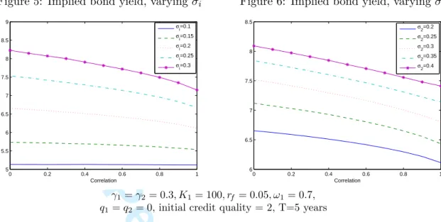
Finally, we consider the impact of varying the volatility of firm-value. Figure 5 shows how yields behave when the volatility of both firms is changed simultaneously. As expected, higher
5 6 7 8 9 10 11 12 13 14 15 16 17 18 19 20 21 22 23 24 25 26 27 28 29 30 31 32 33 34 35 36 37 38 39 40 41 42 43 44 45 46 47 48 49 50 51 52 53 54 55 56 57 58 59 60
For Peer Review Only
Figure 5: Implied bond yield, varyingσi
0 0.2 0.4 0.6 0.8 1 5 5.5 6 6.5 7 7.5 8 8.5 9 Correlation σi=0.1 σi=0.15 σi=0.2 σi=0.25 σi=0.3
Figure 6: Implied bond yield, varyingσ2
0 0.2 0.4 0.6 0.8 1 6 6.5 7 7.5 8 8.5 Correlation σ 2=0.2 σ2=0.25 σ2=0.3 σ2=0.35 σ 2=0.4 γ1=γ2= 0.3, K1= 100, rf = 0.05, ω1= 0.7,
q1=q2= 0, initial credit quality = 2, T=5 years
volatility leads to a higher likelihood of default and higher yields. In Figure 6 we assume that the volatility of firm one remains fixed at 0.2 yr−1/2 and we increase the volatility in firm
two. Since we are considering the yield on firm one’s bonds, the increasing riskiness of firm two impacts yields through the correlation between the two companies and the possibility of default contagion. As expected, the more volatile firm two is, the riskier firm one and the higher yielding its bonds.
4
CDS Spread Calculations
Using a similar approach to that in Section 3, we evaluate first and second-to-default credit default swap (CDS) spreads for a two-company basket.
4.1 First-to-default CDS Basket
We consider a basket of two related companies. The buyer of a first-to-default CDS on this underlying basket pays a premium, the CDS spread, for the life of the CDS – until maturity or the first default, whichever happens first. In the event of default by one of the underlying reference companies, the buyer receives a default payment and the contract terminates. Denoting the default time of company iby τi, we write τfirst for the time of the
first default,
τfirst= min{τ1, τ2}
where, using the same notation as before,
τi= inf{t:Xi(t) =Bi}.
If bond recovery on default isR, and the protection buyer makes continuous spread payments,
c, on a par value K, then the discounted spread payment (DSP) and discounted default
6 7 8 9 10 11 12 13 14 15 16 17 18 19 20 21 22 23 24 25 26 27 28 29 30 31 32 33 34 35 36 37 38 39 40 41 42 43 44 45 46 47 48 49 50 51 52 53 54 55 56 57 58 59 60
For Peer Review Only
payment (DDP) on the first-to-default basket are DSP = cK Z T 0 e−rfsP(τ first> s) ds DDP = (1−R)K Z T 0 e−rfsP(s≤τ first≤s+ds) ds (7) = (1−R)K Z T 0 − e−rfs ∂ ∂sP(τfirst> s) ds = (1−R)K 1−e−rfTP(τ first > T)−rf Z T 0 e−rfsP(τ first> s) ds .
With P(s) defined as in equation (1), the market spread,cfirst, is therefore
cfirst = (1−R) 1−e−rfTP(τ first> T)− RT 0 rfe−rfsP(τfirst > s) ds RT 0 e−rfsP(τfirst> s) ds (8) = (1−R) 1−e−rfTP(T)−RT 0 rfe−rfsP(s) ds RT 0 e−rfsP(s) ds since P(τfirst> s) =P(τ1> s, τ2> s) =P(X1(s)≥B1, X2(s)≥B2) =P(s). 4.2 Second-to-default CDS Basket
A second-to-default CDS spread is evaluated in the same way. The purchaser of the swap receives a payment in the event that both companies default during the life of the swap, at which point the contract terminates. Denoting τsecond as the time of the second default,
exactly as for (8), the market spread, csecond is
csecond= (1−R) 1−e−rfTP(τ second> T)−R0T rfe−rfsP(τsecond> s) ds RT 0 e−rfsP(τsecond> s) ds , (9) where P(τsecond> s) =P(τ1> s) +P(τ2 > s)−P(τ1> s, τ2> s). (10) 4.3 CDS Basket Results
In Figures 7 - 12, we consider the impact of correlation on first and second-to-default CDS spreads for different parameter values. Numerical evaluation is done by numerical quadrature on a sparse grid as before.
5 6 7 8 9 10 11 12 13 14 15 16 17 18 19 20 21 22 23 24 25 26 27 28 29 30 31 32 33 34 35 36 37 38 39 40 41 42 43 44 45 46 47 48 49 50 51 52 53 54 55 56 57 58 59 60
For Peer Review Only
Figure 7: First-to-default CDS, varying T
−1 −0.5 0 0.5 1 0 0.5 1 1.5 2 2.5 3 Correlation Spread 1 year 2 years 3 years 4 years 5 years
Figure 8: Second-to-default CDS, varying T
−1 −0.5 0 0.5 1 −0.2 0 0.2 0.4 0.6 0.8 1 1.2 Correlation Spread 1 year 2 years 3 years 4 years 5 years σ1=σ2= 0.2, K1= 100, rf = 0.05, q1=q2= 0,
γ1=γ2= 0.03, initial credit quality = 2,R= 0.5
In all cases, with increasing correlation between the two reference entities, first-to-default CDS spreads decrease, whilst second-to-default CDS spreads increase. This is because the proba-bility of at least one company defaulting in a given period is higher for negative correlations, whilst the probability of both defaulting is greater for positive correlations.
Figures 7 and 8 show spreads for first and second-to-default CDS baskets with maturities of up to 5 years. Initial credit quality is 2 (i.e, as before, firm value is initially twice the level of the barrier). Spreads are greater for longer-maturity swaps and, as we would expect, first-to-default spreads are everywhere greater than second-to-default spreads.
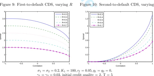
Figure 9: First-to-default CDS, varyingR
−1 −0.5 0 0.5 1 0.5 1 1.5 2 2.5 3 3.5 4 Correlation Spread R=0.3 R=0.4 R=0.5 R=0.6 R=0.7
Figure 10: Second-to-default CDS, varyingR
−1 −0.5 0 0.5 1 0 0.2 0.4 0.6 0.8 1 1.2 1.4 Correlation Spread R=0.3 R=0.4 R=0.5 R=0.6 R=0.7 σ1=σ2= 0.2, K1= 100, rf = 0.05, q1=q2= 0,
γ1=γ2= 0.03, initial credit quality = 2, T = 5
Figures 9 and 10 illustrate the extent to which CDS spreads depend on our recovery rate as-sumption. As would be expected, moving from a 30% recovery rate to a 70% recovery rate has a large impact. However, the overall form of spreads and their variation with changing cor-relation is the same. In general, taking R=50% is representative of the levels seen in practice
6 7 8 9 10 11 12 13 14 15 16 17 18 19 20 21 22 23 24 25 26 27 28 29 30 31 32 33 34 35 36 37 38 39 40 41 42 43 44 45 46 47 48 49 50 51 52 53 54 55 56 57 58 59 60
For Peer Review Only
(see, for example, Bakshi et al. (2006)) and is in line with that used in the CreditGradesT M approach to modelling credit as described in Finger et al. (2002). An easy extension would be to set the recovery rate of the reference entities equal to discounted par value.
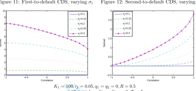
Figure 11: First-to-default CDS, varying σi
−1 −0.5 0 0.5 1 0 1 2 3 4 5 6 7 8 9 10 Correlation Spread σi=0.1 σi=0.15 σi=0.2 σi=0.25 σi=0.3
Figure 12: Second-to-default CDS, varyingσi
−1 −0.5 0 0.5 1 −0.5 0 0.5 1 1.5 2 2.5 3 Correlation Spread σi=0.1 σi=0.15 σi=0.2 σi=0.25 σi=0.3 K1= 100, rf = 0.05, q1=q2= 0, R= 0.5
γ1=γ2= 0.03, initial credit quality = 2, T = 5
Figures 11 and 12 show that firm volatility has a considerable impact on spreads. As the reference entities become more volatile, both credit default swaps become much more risky and spreads increase significantly. Of all the parameters, firm volatility has by far the largest impact on CDS spreads.
Through implementation of the analytical formula for the joint survival probability function, (1), we are therefore able to illustrate the sensitivity of first and second-to-default CDS spreads to input parameter assumptions straightforwardly. The importance of the degree of correlation between reference entities is clearly evident, with spreads significantly different when the basket is highly correlated than when it is well diversified.
Since by definition default contagion comes into play following the first default, its existence has no impact on first-to-default spreads. It is, however, important in the consideration of second-to-default spreads, and introducing the default contagion mechanism considered in Section 3 clearly has a dramatic impact on second-to-default spreads, in this case making them equal to first-to-default spreads. This situation is clearly extreme, as a CDS is highly unlikely to be constructed on such an undiversified basket (unless of course the existence of the link between firms was completely unknown prior to the first default), however it serves to highlight the importance of considering the dependence relationship between firms.
4.4 CDS with Counterparty Risk
Consider now a single-name CDS, face-value K, maturity T, on reference company one bought from a counterparty company two. The purchaser of the CDS makes spread payments for the life of the CDS – until either the reference company or the counterparty defaults. If the reference entity defaults during the life of the CDS and before the counterparty, the purchaser receives a default payment. If, however, the counterparty defaults first, they receive nothing,
5 6 7 8 9 10 11 12 13 14 15 16 17 18 19 20 21 22 23 24 25 26 27 28 29 30 31 32 33 34 35 36 37 38 39 40 41 42 43 44 45 46 47 48 49 50 51 52 53 54 55 56 57 58 59 60
For Peer Review Only
irrespective of whether or not the reference company later defaults. Denoting the default time of company i by τi, if bond recovery on default is R and the purchaser of protection
makes continuous spread payments, c, for the life of the CDS, then using the same notation as before, the protection buyer
• makes spread payments for t <min{τ1, τ2, T}, • receives a default payment if τ1 <min{τ2, T}, • receives nothing if τ2<min{τ1, T}.
In other words, discounted spread and default payments are
Spread = cK Z T 0 e−rfsP(τ 1 > s, τ2 > s) ds = cK Z T 0 e−rfsP(X 1(s)≥B1, X2(s)≥B2) ds Default = (1−R)K Z T 0 e−rfsP(s≤τ 1 ≤s+ds, τ2 > s) ds
Considering the default payment for a first-to-default CDS, equation (7),
DDP = (1−R)K Z T 0 e−rfsP(s≤τ first≤s+ds) ds (11) = (1−R)K Z T 0 e−rfs P(s≤τ1 ≤s+ds, τ2 > s) +P(τ1> s, s≤τ2 ≤s+ds) ds,
we see that the default payment for a CDS with counterparty, added to its image when the identity of the reference entity and the counterparty are swapped, gives the value of the first-to-default swap payment. A similar identity holds for the second-first-to-default swap payment. In the case of a homogeneous portfolio, when both reference entities have the same parameters, (11) can be used to calculate the value of a CDS spread with counterparty risk for all values of correlation,ρ. More generally, in the asymmetric case a more complicated evaluation must be done, details of which will be considered elsewhere.
5
Conclusion
Structural models are increasingly the focus of industry attention in the multi-firm setting, but there has been limited work on the general first passage framework, and little academic coverage. This paper makes a first and novel, albeit by necessity simplistic, contribution to this field through the introduction of a contagion mechanism in a two-dimensional first passage model. Working with a Black and Cox (1976) type structural framework, we have built on the work by Zhou (2001) to derive analytical formulae for both bond yields and CDS spreads. We have modified the default barrier to better reflect reality and have incorporated
6 7 8 9 10 11 12 13 14 15 16 17 18 19 20 21 22 23 24 25 26 27 28 29 30 31 32 33 34 35 36 37 38 39 40 41 42 43 44 45 46 47 48 49 50 51 52 53 54 55 56 57 58 59 60
For Peer Review Only
default contagion within the structural framework for the first time. The result is a credit model that is asymmetric with respect to default risk and which has a dependence structure based on both long-term asset correlation and default contagion.
Results illustrate that the sensitivity of yields to input parameters is as expected, and clearly demonstrate the importance of credit correlation. Our model enables us to generate corporate bond yields and CDS spreads across the full range of parameter values in a two-dimensional first passage framework in full generality. This has not been done before. Previous results using related analysis in Zhou (2001) (default correlations) and Hua et al. (1998) (double lookbacks) have concentrated on cases in which the framework simplifies and have been lim-ited to a few parameter values in these cases. For the first time, we are therefore able to fully consider spread sensitivity to model and parameter assumptions in the two-dimensional structural setting.
Our specification of default contagion is clearly not very realistic – default by one company very rarely leads to direct default by another, although it is possible. More likely, the im-pact of a corporate bankruptcy causes a ripple of credit weakness through the market as related companies are impacted.10 Nonetheless, the importance of taking into account credit interactions is, once again, clearly highlighted.
Dependence modelling is most critical in the analysis and pricing of large basket credit deriva-tives, such as kth-to-default credit default swap baskets and CDO tranches. These require the framework to be extended to considerably more than two dimensions. This is an area of current research interest and is not straightforward since analytical formulae are no longer possible and numerical solutions become highly problematic with increasing dimension. As intimated in Section 3, it would be attractive to incorporate a network of asymmetric depen-dences within a portfolio, enabling the impact of a credit event at one company to cause a ripple of contagion through other, related, parties.
A
Derivation of Maturity Payment
For ease of notation, we denote the joint survival probability transition density
p(x1, x2, t) = ∂2 ∂x1∂x2P
(X1(t)≤x1, X2(t)≤x2, X1(t)≥B1, X2(t)≥B2)
Proposition A.1 For general A and B,
Z ∞ B2 Z B A ex1p(x 1, x2, t) dx1dx2 = 2 βte (a1+)B1+a2B2+bt ∞ X n=1 e−r02/2tsin nπθ0 β Z β 0 sin nπθ β gn(θ) dθ
10We address this numerically in a subsequent paper, Haworth and Reisinger (2006), however analytical
solutions are no longer possible. 5 6 7 8 9 10 11 12 13 14 15 16 17 18 19 20 21 22 23 24 25 26 27 28 29 30 31 32 33 34 35 36 37 38 39 40 41 42 43 44 45 46 47 48 49 50 51 52 53 54 55 56 57 58 59 60
For Peer Review Only
where gn(θ) = Z dB dA re−r2/2t e[A(θ)+σ1sin(β−θ)]rI (nπ β ) rr0 t dr r0 = 1 p 1−ρ2 B21 σ12 − 2ρB1B2 σ1σ2 +B 2 2 σ22 1/2 tanθ0 = σ1B2 p 1−ρ2 σ2B1−ρσ1B2 , θ0∈[0, β] dA = A−B1 σ1 hp 1−ρ2cosθ+ρsinθi dB = B−B1 σ1 hp 1−ρ2cosθ+ρsinθi A(θ) = a1σ1sin(β−θ) +a2σ2sinθ, ProofUsing notation from Section 2, by Hua et al. (1998)
p(x1, x2, t) = 2ea1x1+a2x2+bt βtσ1σ2 p 1−ρ2 ∞ X n=1 e−(r2+r20)/2tsin nπθ0 β sin nπθ β I(nπ β ) rr0 t . Changing variables, x1 = B1+ p (1−ρ2)σ 1rcosθ+ρσ1rsinθ (12) x2 = B2+σ2rsinθ,
the Jacobian for the transformation isp(1−ρ2)rσ
1σ2, and Z ∞ B2 Z B A ex1p(x 1, x2, t) dx1dx2 = 2 βte (a1+)B1+a2B2+bt ∞ X n=1 e−r20/2tsin nπθ0 β Z θ sin nπθ β gn(θ) dθ where gn(θ) = Z r re−r2/2te[A(θ)+σ1sin(β−θ)]rI (nπ β ) rr 0 t dr, since
cosβ =−ρ & sinβ =p1−ρ2.
WritingX= x1−B1 σ1 and Y = x2−B2 σ2 then from (12), X = rhp(1−ρ2) cosθ+ρsinθi (13) Y = rsinθ 6 7 8 9 10 11 12 13 14 15 16 17 18 19 20 21 22 23 24 25 26 27 28 29 30 31 32 33 34 35 36 37 38 39 40 41 42 43 44 45 46 47 48 49 50 51 52 53 54 55 56 57 58 59 60
For Peer Review Only
Since 0≤ A−B1 σ1 ≤ X≤ B−B1 σ1 0 ≤ Y ≤ ∞ it follows that tanθ= p 1−ρ2 X/Y −ρ, ⇒ θ∈[0, β] and letting dA= A−B1 σ1 hp 1−ρ2cosθ+ρsinθi dB= B−B1 σ1 hp 1−ρ2cosθ+ρsinθi,we havedA≤r≤dB from (13). The result follows.
Derivation of Maturity Payment
From Section 3, the discounted maturity payment, DMP, is: DMP = e−rfT Z ∞ B2 Z ∞ d K1p(x1, x2, T) dx1dx2 (14) +e−rfT Z ∞ B2 Z d B1 ω1V1(0)ex1+γ1Tp(x1, x2, T) dx1dx2 (15)
Using Proposition (A.1) with= 0, A =d and B =∞ for line (14) and= 1,A =B1 and B=dfor line (15), the payment on maturity becomes:
DMP = H1(T) ∞ X n=1 sin nπθ0 β Z β 0 sin nπθ β g+n(θ) dθ +H2(T) ∞ X n=1 sin nπθ0 β Z β 0 sin nπθ β g∗n(θ) dθ 5 6 7 8 9 10 11 12 13 14 15 16 17 18 19 20 21 22 23 24 25 26 27 28 29 30 31 32 33 34 35 36 37 38 39 40 41 42 43 44 45 46 47 48 49 50 51 52 53 54 55 56 57 58 59 60
For Peer Review Only
where, H1(T) = 2K1e−rfT βT e a1B1+a2B2+bTe−r20/2T H2(T) = 2ω1V1(0)e(γ1−rf)T βT e (a1+1)B1+a2B2+bTe−r02/2T gn+(θ) = Z ∞ d∗(θ) re−r2/2TeA(θ)rI(nπ β ) rr0 T dr gn∗(θ) = Z d∗(θ) 0 re−r2/2Te[A(θ)+σ1sin(β−θ)]rI (nπ β ) rr0 T dr d∗(θ) = d−B1 σ1 hp 1−ρ2cosθ+ρsinθi = lnω1 σ1sin(θ−β) ≥ 0.References
G. Bakshi, D. Madan, and F. Zhang. Recovery risk in defaultable debt models: empirical comparisons and implied recovery rates. Working Paper, University of Maryland, 2006.
http://www.fdic.gov/bank/analytical/cfr/2006/apr/cfrss 2006 Bakshi.pdf.
M. Baxter. Dynamic modelling of single-name credits and CDO tranches. Nomura Fixed Income Quant Group, 2006.
http://www.nomura.com/resources/europe/pdfs/cdomodelling.pdf.
F. Black and J. Cox. Valuing corporate securities: Some effects of bond indenture provisions.
Journal of Finance, 31:351–367, 1976.
U. Cherubini, E. Luciano, and W. Vecchiato. Copula methods in finance. Wiley, 2004. C. Finger, V. Finkelstein, G. Pan, J. Lardy, T. Thomas, and J. Tierney. CreditgradesT M.
Technical Document, RiskMetrics Group, Inc., 2002.
http://www.creditgrades.com/resources/pdf/CGtechdoc.pdf.
M. Genest and B. Remillard. Discussion of ‘Copulas: Tales and Facts’, by Thomas Mikosch.
Extremes, 9:27–36, 2006.
T. Gerstner and M. Griebel. Numerical integration using sparse grids. Numerical Algorithms, 18:209–332, 1998.
K. Giesecke. Credit risk modeling and valuation: An introduction. Working Paper, Cornell University, 2004.
http://www.stanford.edu/dept/MSandE/people/faculty/giesecke/introduction.pdf. H. Haworth. Structural models of credit with default contagion. DPhil Thesis, 2006.
http://eprints.maths.ox.ac.uk/554/01/haworth.pdf.
H. Haworth and C. Reisinger. Modeling basket credit default swaps with default contagion.
6 7 8 9 10 11 12 13 14 15 16 17 18 19 20 21 22 23 24 25 26 27 28 29 30 31 32 33 34 35 36 37 38 39 40 41 42 43 44 45 46 47 48 49 50 51 52 53 54 55 56 57 58 59 60
For Peer Review Only
Working paper, Oxford University, 2006.
http://eprints.maths.ox.ac.uk/561/01/HaworthReisinger.pdf.
H. Hua, W.P. Keirstead, and J. Rebholz. Double lookbacks.Mathematical Finance, 8:201–228, July 1998.
J. Hull, M. Predescu, and A. White. The valuation of correlation-dependent credit derivatives using a structural model. Working Paper, University of Toronto, 2005.
http://www.rotman.utoronto.ca/~hull/DownloadablePublications/StructuralModel.pdf. J. Hull and A. White. Valuing credit default swaps II: Modeling default correlations. Journal
of Derivatives, 8 No. 3:12–22, 2001.
R. Jarrow and J. Yu. Counterparty risk and the pricing of defaultable securities.The Journal of Finance, LVI No. 5:1765–1800, 2001.
D. Lando. Credit Risk Modeling: Theory & Applications. Princeton University Press, 2004. E. Luciano and W. Schoutens. A multivariate jump-driven financial asset model. ICER
Working Paper, 2005.
http://perswww.kuleuven.be/~u0009713/multivg.pdf.
R. Merton. On the pricing of corporate debt: The risk structure of interest rates. Journal of Finance, 29:449–470, 1974.
T. Mikosch. Copulas: Tales and Facts. Extremes, 9:3–20, 2006.
T. Moosbrucker. Explaining the correlation smile using Variance Gamma distributions. The Journal of Fixed Income, 16:71–87, 2006.
P.J. Sch¨onbucher. Credit derivatives pricing models. Wiley, 2003.
C. Zhou. An analysis of default correlations and multiple defaults. The Review of Financial Studies, 14:555–576, 2001. 5 6 7 8 9 10 11 12 13 14 15 16 17 18 19 20 21 22 23 24 25 26 27 28 29 30 31 32 33 34 35 36 37 38 39 40 41 42 43 44 45 46 47 48 49 50 51 52 53 54 55 56 57 58 59 60