CEC Theses and Dissertations College of Engineering and Computing
2016
Evaluation of Supervised Machine Learning for
Classifying Video Traffic
Farrell R. Taylor
Nova Southeastern University,[email protected]
This document is a product of extensive research conducted at the Nova Southeastern UniversityCollege of Engineering and Computing. For more information on research and degree programs at the NSU College of Engineering and Computing, please clickhere.
Follow this and additional works at:http://nsuworks.nova.edu/gscis_etd
Part of theArtificial Intelligence and Robotics Commons
Share Feedback About This Item
This Dissertation is brought to you by the College of Engineering and Computing at NSUWorks. It has been accepted for inclusion in CEC Theses and Dissertations by an authorized administrator of NSUWorks. For more information, please [email protected].
NSUWorks Citation
Farrell R. Taylor. 2016.Evaluation of Supervised Machine Learning for Classifying Video Traffic.Doctoral dissertation. Nova Southeastern University. Retrieved from NSUWorks, College of Engineering and Computing. (972)
Evaluation of Supervised Machine Learning for Classifying Video
Traffic
by Farrell Taylor
A dissertation submitted in partial fulfillment of the requirements for the degree of Doctor of Philosophy
in
Information Systems
Graduate School of Computer and Information Sciences Nova Southeastern University
We hereby certify that this dissertation, submitted by Farrell Taylor, conforms to acceptable standards and is fully adequate in scope and quality to fulfill the dissertation requirements for the degree of Doctor of Philosophy.
_____________________________________________ ________________ Sumitra Mukherjee , Ph.D. Date
Chairperson of Dissertation Committee
_____________________________________________ ___________ _____ Michael J. Laszlo, Ph. D . D ate
Dissertation Committee Member
_____________________________________________ ________________ Gregory E. Simco , Ph.D. Date
Dissertation Committee Member
Approved:
_____________________________________________ __ ______________ Ronald J. Chenail, Ph.D. Date
An Abstract of a Dissertation Submitted to Nova Southeastern University in Partial Fulfillment of the Requirements for the Degree of Doctor of Philosophy
Evaluation of Supervised Machine Learning for Classifying Video
Traffic
by Farrell Taylor
May 2016
Operational deployment of machine learning based classifiers in real-world networks has become an important area of research to support automated real-time quality of service decisions by Internet service providers (ISPs) and more generally, network
administrators. As the Internet has evolved, multimedia applications, such as voice over Internet protocol (VoIP), gaming, and video streaming, have become commonplace. These traffic types are sensitive to network perturbations, e.g. jitter and delay. Automated quality of service (QoS) capabilities offer a degree of relief by prioritizing network traffic without human intervention; however, they rely on the integration of real-time traffic classification to identify applications. Accordingly, researchers have begun to explore various techniques to incorporate into real-world networks. One method that shows promise is the use of machine learning techniques trained on sub-flows – a small number of consecutive packets selected from different phases of the full application flow.
Generally, research on machine learning classifiers was based on statistics derived from full traffic flows, which can limit their effectiveness (recall and precision) if partial data captures are encountered by the classifier. In real-world networks, partial data captures can be caused by unscheduled restarts/reboots of the classifier or data capture
capabilities, network interruptions, or application errors. Research on the use of machine learning algorithms trained on sub-flows to classify VoIP and gaming traffic has shown promise, even when partial data captures are encountered. This research extends that work by applying machine learning algorithms trained on multiple sub-flows to classification of video streaming traffic.
Results from this research indicate that sub-flow classifiers have much higher and more consistent recall and precision than full flow classifiers when applied to video traffic. Moreover, the application of ensemble methods, specifically Bagging and adaptive boosting (AdaBoost) further improves recall and precision for sub-flow classifiers. Findings indicate sub-flow classifiers based on AdaBoost in combination with the C4.5 algorithm exhibited the best performance with the most consistent results for
Acknowledgements
It has been a long journey to this point, filled with numerous challenges; however, looking back, the endeavor was well worth the effort. When I first entered the program, I was told that a PhD is a personal journey that should not be undertaken for career, financial gain, nor ego. This was sage advice.
Several friends have been supportive of my efforts to attain a PhD. Dr. Dennis Bauer, a dear friend and colleague who provided an emotional push to move me from the point of indecision to commitment. Also, Dr. Dolly Mastrangelo, who provided encouragement at a key point in this journey when I strongly considered stopping my pursuit of a PhD. I owe Dr. Mastrangelo a great deal of thanks. To Zachary Parker, who spent his time discussing and providing reviews on a subject that had very little interest to him, and simply being there when needed, thank you. I would like to thank Dr. Stephen Dinkle for his advice and mentorship from the beginning of my PhD program until its completion. Dr. Dinkel’s reviews and advise throughout this process was instrumental to my success. To my dissertation committee, Dr. Sumitra Mukherjee, Dr. Michael Laszlo and Dr.
Gregory Simco, I would like to extend appreciation and gratitude for their guidance and support. A very special thanks to Dr. Sumitra Mukherjee. Dr. Mukherjee was and still is a motivating force for me undertaking and completing my dissertation. Dr. Mukherjee is simply one of the best professors, more importantly, “teachers”, I have ever had, and as he’s done for me, will continue to inspire other students to achieve.
Finally, I would like to thank my wife, Toni, who has supported me throughout this process. Many nights, weekends and in some cases mini-vacations where sacrificed for this work. I owe her a sincere debt of gratitude. And to my children; the greatest achievement I have ever made is being a father. Thank you Mackenzie, Elyse and Samantha for calling me “Dad”.
iii Table of Contents Abstract ii Acknowledgements iii List of Tables v List of Figures vi Chapters 1. Introduction 1 Background 1 Problem Statement 4 Dissertation Goal 4 Research Questions 5 Relevance and Significance 6 Barriers and Issues 8
Definition of Terms 9 Summary 11
2. Review of the literature 12
Introduction 12
Initial Approaches to IP Traffic Classification 12 IP Classification using Unsupervised ML 13 IP Classification using Supervised ML 15
IP Classification using Semi-Supervised (Hybrid) ML 17 Operationalizing ML Classifiers 17
ML Techniques Applied in this Research 19 Support Vector Machine 22
Naïve Bayes 27 C4.5 31
Ensemble Techniques used to Improve ML Performance 38 Summary 41
3. Methodology 42
Introduction 42
Step 1 – Data Collection 43 Step 1a – Capturing Live Traffic 44
Step 1b – Generating Full Flow and Sub-flow Feature Sets 45 Step 1c – Creating Training and Test Sets 48
Step 2 – Classification Based on Full Flows 49 Step 3 – Classification Based on Sub-flows 50
Evaluating Ensemble Techniques: Bagging and Boosting 51 Format for Results 52
Resource Requirements 53 Summary 53
iv
4. Results 55
Data Preprocessing 55
Addressing Class Imbalance 57
Full Flow Trained Classifier Applied to Partial Flows with Missing Packets 58 J48 C4.5 Full Flow Classifier Performance 59
Naïve Bayes Full Flow Classifier Performance 63 SVM Full Flow Classifier Performance 67 Summary 71
Sub-flow Trained Classifiers Applied to Partial Flows with Missing Packets 72 Sub-flow “m0,n25,s10” Model Evaluation 73
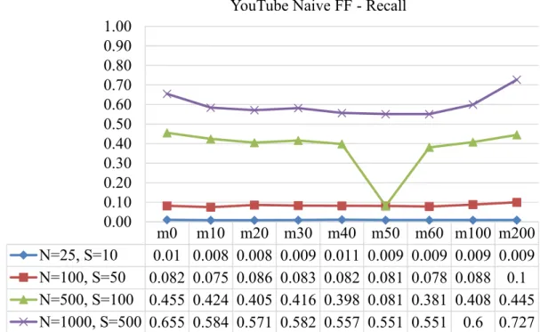
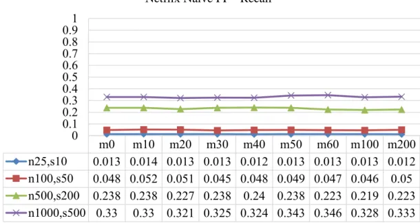
Sub-flow “m0,n100,s50” Model Evaluation 77 Sub-flow “m0,n500,s200” Model Evaluation 82 Sub-flow “m0,n1000,s500” Model Evaluation 86 Summary 90
Evaluation of Ensemble Algorithms Applied to Sub-flow Classifiers 91 YouTube Sub-flow Bagging Classifiers 91
YouTube Sub-flow ADA Classifiers 95 Netflix Sub-flow Bagging Models 98 Netflix Sub-flow AdaBoost Classifiers 101 Summary 105
5. Conclusions, Implications, Recommendations, and Summary 106
Conclusion 106 Implications 109 Recommendations 109 Summary 110
v
List of Tables Tables
1. Table 1 Definition of Terms 9
2. Table 2 Full Flow and Sub-flow Statistics 46
3. Table 3 Required Resources 53
4. Table 4 YouTube Dataset 56
5. Table 5 Netflix Dataset 56
6. Table 6 Full Flow Training Stats 59
7. Table 7 YouTube m0,n25,s10 Model Results 74
8. Table 8 Netflix m0,n25,s10 Model Results 75
9. Table 9 YouTube m0,n100,s50 Model Results 78
10. Table 10 Netflix m0,n100,s50 Model Results 80
11. Table 11 YouTube m0,n500,s200 Model Results 82
12. Table 12 Netflix m0,n500,s200 Model Results 84
13. Table 13 YouTube m0,n1000,s500 Model Results 86
14. Table 14 Netflix m0,n1000,s500 Model Results 88
15. Table 15 YouTube Bagging-J48 Results 92
16. Table 16 YouTube Bagging-Naive Results 93
17. Table 17 YouTube Bagging-SMO Results 94
18. Table 18 YouTube ADA-J48 Results 95
19. Table 19 YouTube ADA-Naive Results 97
20. Table 20 YouTube ADA-SMO Results 98
21. Table 21 Netflix Bag-J48 Results 99
22. Table 22 Netflix Bag-Naive Results 100
23. Table 23 Netflix Bag-SMO Results 101
24. Table 24 Netflix ADA-J48 Results 102
25. Table 25 Netflix ADA-Naive Results 103
vi
List of Figures Figures
1. Figure 1 Generalized Depiction of Machine Learning 20
2. Figure 2 Linear Support Vector Machine 24
3. Figure 3 Overview of Research Methodology 43
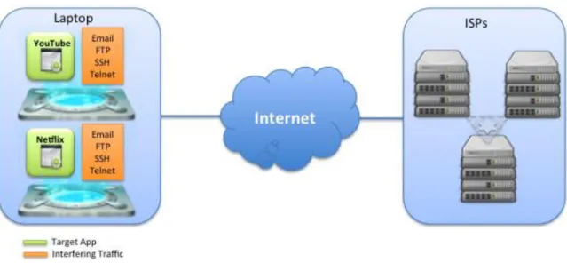
4. Figure 4 Environment used to Capture Traffic 44
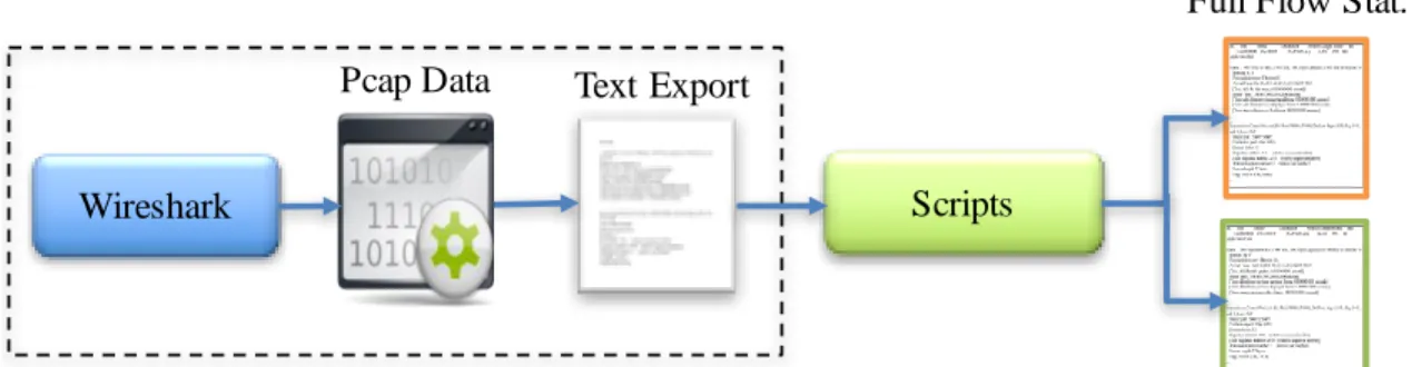
5. Figure 5 Generating Full and Sub-flow Statistics 46
6. Figure 6 Sample Wireshark Text Export 48
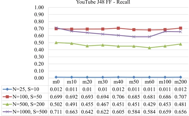
7. Figure 7 Recall for YouTube J48 Full-flow Classifier Tested with Partial Flows 60
8. Figure 8 Recall for Netflix J48 Full-flow Classifier Tested with Partial Flows 60
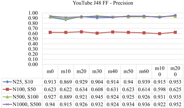
9. Figure 9 Precision for YouTube J48 Full-flow Classifier Tested with Partial Flows 62
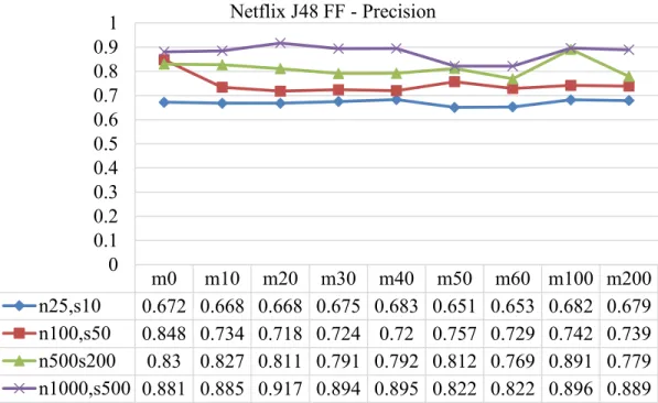
10. Figure 10 Precision for Netflix J48 Full-flow Classifier Tested with Partial Flows 63
11. Figure 11 Recall for YouTube Naïve Bayes Full-flow Classifier Tested with Partial Flows 64
12. Figure 12 Recall for Netflix Naïve Bayes Full-flow Classifier Tested with Partial Flows 65
13. Figure 13 Precision for YouTube Naïve Bayes Full-flow Classifier Tested with Partial Flows 66
14. Figure 14 Precision for Netflix Naïve Bayes Full-flow Classifier Tested with Partial Flows 67
15. Figure 15 Recall for YouTube SVM Full-flow Classifier Tested with Partial Flows 69
16. Figure 16 Recall for Netflix SVM Full-flow Classifier Tested with Partial Flows 69
17. Figure 17 Precision for YouTube SVM Full-flow Classifier Tested with Partial Flows 70
18. Figure 18 Precision for Netflix SVM Full-flow Classifier Tested with Partial Flows 71
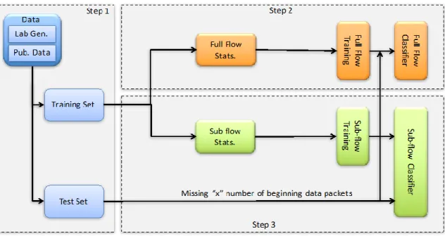
19. Figure 19 Process for Evaluating Sub-flow Models 72
20. Figure 20 YouTube J48 m0,n25,s10 Model 74
21. Figure 21 YouTube Naive m0,n25,s10 Model 75
22. Figure 22 YouTube SMO m0,n25,s10 Model 75
23. Figure 23 Netflix J48 m0,n25,s10 Results 76
24. Figure 24 Netflix Naive m0,n25,s10 Results 77
25. Figure 25 Netflix SMO m0,n25,s10 Results 77
26. Figure 26 YouTube J48 m0,n100,s50 Results 79
27. Figure 27 YouTube Naive m0,n100,s50 Results 79
28. Figure 28 YouTube SMO m0,n100,s50 Results 80
29. Figure 29 Netflix J48 m0,n100,s50 Model 81
30. Figure 30 Netflix Naïve m0,n100,s50 Model 81
31. Figure 31 Netflix m0,n100,s50 Model 82
32. Figure 32 J48 m0,n500,s200 Model 83
33. Figure 33 Netflix Naïve m0,n500,s200 Model 83
34. Figure 34 Netflix SMO m0,n500,s200 Model 84
35. Figure 35 Netflix J48 m0,n500,s200 Model 85
vii 37. Figure 37 Netflix SMO m0,n500,s200 Model 86
38. Figure 38 YouTube J48 m0,n1000,s500 Model 87
39. Figure 39 YouTube Naive m0,n1000,s500 Model 87
40. Figure 40 YouTube SMO m0,n1000,s500 Model 88
41. Figure 41 Netflix J48 m0,n1000,s500 Model 89
42. Figure 42 Netflix Naive m0,n1000,s500 Model 90
43. Figure 43 Netflix SMO m0,n1000,s500 Model 90
44. Figure 44 YouTube Bagging-J48 F-Measure 93
45. Figure 45 YouTube Bagging-Naive F-Measure 94
46. Figure 46 YouTube Bagging-Naive F-Measure 95
47. Figure 47 YouTube ADA-J48 F-Measure 96
48. Figure 48 YouTube ADA-Naive F-Measure 97
49. Figure 49 YouTube ADA-SMO F-Measure 98
50. Figure 50 Netflix Bag-J48 F-Measure 99
51. Figure 51 Netflix Bag-Naive F-Measure 100
52. Figure 52 Netflix Bag-SMO F-Measure 101
53. Figure 53 Netflix ADA-J48 F-Measure 103
54. Figure 54 Netflix ADA-Naive F-Measure 104
Chapter 1
Introduction
Background
Internet Protocol (IP) network traffic classification is a key objective of internet service providers (ISPs) and network administrators supporting decisions related to quality of service (QoS), security, traffic shaping and overall network management (Dainotti, Pescape, & Claffy, 2012; Nguyen & Armitage, 2008). Traffic classification is the practice of correlating network flows to the applications that generated them (Mu & Wu, 2011). Initially, IP traffic classification was accomplished through the examination of common characteristics of network packets such as IP address, well-known ports and payload inspection (Karagiannis, Papagiannaki, & Faloutsos, 2005). Well-known ports were the preeminent means of identifying traffic (i.e. traffic classification) based on the Internet Assigned Numbers Authority (IANA) application port registration and were integrated into network monitoring tools such as NetFlow and sflow (Zander, Nguyen, & Armitage, 2005). Payload inspection, also referred to as deep-packet inspection, was a complementary technique, based on content analysis of the data portion of an IP packet (Bernaille, Teixeira, Akodkenou, Soule, & Salamatian, 2006). Both methodologies produced early success in classifying network flows to the applications that originated the traffic (Bernaille et al., 2006; Moore & Papagiannaki, 2005).
Although techniques based on well-known ports and payload inspection realized a level of success, today’s network applications, especially peer to peer (P2P), have become more sophisticated and the reliance on these characteristics to identify specific application protocols is suspect (Soysal & Schmidt, 2010; Yuan, Li, Guan, & Xu, 2010).
P2P applications (e.g. gaming, video streaming, voice over IP (VoIP)) may use a variety of ports to communicate between end user devices and servers, and payload inspection can be computationally expensive, infringe on privacy laws by revealing user content and could be rendered ineffective if encryption is used (Karagiannis, Broido, Faloutsos, & claffy, 2004; Yibo, Dawei, & Luoshi, 2013). Moreover, users have begun to purposely evade detection using encryption, tunnels, and ephemeral ports (Karagiannis et al., 2004).
To address deficiencies associated with using port and payload inspection for traffic identification researchers have applied machine learning techniques – based on network flow statistics – to support classification of IP traffic (Callado et al., 2009; Zander et al., 2005). Generally, a flow is defined by a sequence of five-tuples: source IP, destination IP, source port, destination port, and protocol (Dainotti et al., 2012; Hu, Chiu, & Lui, 2009). Overall results have been promising; however, several research worthy areas remain; in particular, research on the operational deployment of classifiers in real-world networks to identify P2P interactive traffic (Li, Springer, Bebis, & Hadi Gunes, 2013; Nguyen & Armitage, 2008). Deploying classifiers into real-world networks is a key aspect of
automating QoS decisions to enable immediate, without the need for human intervention, reprioritization of network traffic to support real-time Internet applications (McGregor, Hall, Lorier, & Brunskill, 2004).
Operational deployment of machine learning (ML) based classifiers have several challenges: timely and continuous classification, directional neutrality, efficient use of memory, portability and robustness (Nguyen & Armitage, 2008). Nguyen, Armitage, Branch, and Zander (2012) developed a means to address a key challenge associated with real-time classifiers, specifically, the challenges associated with timeliness and
continuous classification of traffic flows. Nguyen et al. (2012) methodology uses sub-flows – fragments of full traffic sub-flows containing some number of contiguous packets – for identification of IP flows that addressed timeliness and continuous classification challenges. Prior to this work, the majority of the research on IP traffic classification used statistics derived from the entire traffic flow (Nguyen & Armitage, 2006). However, real-time classifiers may encounter partial, incomplete, traffic flows for a number of reasons: unscheduled shutdown/reboots of packet capture capabilities, network interruptions, or application errors (Nguyen & Armitage, 2006). Nguyen et al. (2012) found that
classifiers trained on statistics from full flows, and used to identify flows from partial, incomplete network traffic captures where initial packets are missing, exhibited degraded performance in terms of recall and precision. Conversely, classifiers trained on multiple sub-flows across the entire life of the application performed well -- better than 95% for both recall and precision – even if the data being analyzed did not represent complete captures of the entire application session. Additionally, sub-flows represent a small portion of the entire flow of traffic, consequently less processing is needed to generate flow statistics, train, and perform classification of the target network traffic. Although Nguyen et al. (2012) were successful in applying this methodology, their work focused on the identification of two specific applications: Wolfenstein: Enemy Territory and VoIP. This research extends (Nguyen et al., 2012) work by evaluating the performance, in terms of recall and precision, of supervised machine learning algorithms trained on sub-flows in identifying video streaming traffic (i.e. YouTube and Netflix).
Problem Statement
Deployment of traffic classifiers in real-world networks has several challenges: timely and continuous classification, directional neutrality, efficient use of memory, and portability and robustness (Nguyen & Armitage, 2008). Of particular interest to this research is the challenge associated with timely and continuous classification of IP traffic. “A timely classifier should reach its decision using as few packets as possible from each flow (rather than waiting until each flow completes before reaching a decision)” (Nguyen & Armitage, 2008, p. 63). Additionally, it is not adequate to require the beginning
packets of a traffic flow to produce high recall and precision– good classifier performance. In reality, network flows captured from real-world networks may be incomplete, due to unscheduled restarts of monitoring capabilities, network interruption, or application errors (Nguyen & Armitage, 2006; Nguyen et al., 2012; Zander, Nguyen, & Armitage, 2012). Moreover, packet statistics may change over the lifetime of an application’s flow, e.g. initial client server negotiation vice established connection between client and server. Accordingly, classifiers must be able to continuously classify
traffic throughout the lifetime of the application’s flow (Nguyen & Armitage, 2008). The problem studied for this research effort is the timely and continuous
classification of video streaming traffic using ML based classifiers trained on multiple sub-flows, when partial, incomplete data sets are encountered.
Dissertation Goal
The goal of this research is to evaluate the effectiveness, specifically recall and precision, of ML techniques trained on sub-flows to classify video streaming traffic. Three ML algorithms are used – C4.5, Naïve Bayes, and Support Vector Machine (SVM)
– to address this goal. C4.5 and Naïve Bayes were used as part of the original work by Nguyen et al. (2012) and Nguyen and Armitage (2006) with good results; thusly, these methods are expected to be well suited to support this research effort. SVM has also been applied successfully in previous work for classification of network traffic (Este, Gringoli, & Salgarelli, 2009; Yuan et al., 2010). Additionally, ensemble techniques were considered, combining the outputs of each ML algorithm in order to enhance the
performance of any single classifier (Dong & Han, 2005; Jianli & Yuncai, 2012). This research effort expands knowledge on using ML techniques to classify IP network traffic toward enabling the timely and continuous classification in real-world network
environments.
Research Questions
This research answers the following questions:
1) What recall and precision can be attained using ML algorithms trained on multiple sub-flows in classifying video streaming traffic?
2) What sub-flow sized is needed to train, test and classify video traffic to attain high recall and precision?
3) What features, sub-flow attributes, are required to enable classification of video traffic?
4) What is the effect of different sub-flow sizes, number of packets per sub-flow, on ML recall and precision?
5) How effective are ML algorithms trained on multiple sub-flows in classifying video streaming traffic from disparate data sets containing packets captured from different network environments?
Relevance and Significance
In the early days of the Internet, data was transmitted on the basis of best effort (Xipeng & Ni, 1999). Nowadays, the Internet has become a platform for provisioning complex multimedia application services such as online gaming, e-commerce, video (streaming and interactive), VoIP, Internet radio, and large-scale file sharing (Roughan, Sen, Spatscheck, & Duffield, 2004). Additionally, with the advent of mobile devices, which ushered in the era of ubiquitous network access, the Internet has seen exponential growth (Roughan et al., 2004). “At the current pace of growth, Internet traffic is doubling approximately every two years, leading to a factor of 1000 growth in the next two
decades” (Saleh & Simmons, 2011, p. 132).
As demand for Internet services has steadily increased, so has ISPs desire for detailed understanding of the various applications traversing their networks to support real-time network management (Jin et al., 2012). Content providers, understanding the importance of provisioning high-quality application services, are keenly interested in assured services to support a competitive advantage in their respective markets (Meddeb, 2010). The confluence of these challenges has provided ISPs with a new business
opportunity where differentiated services, in the form of QoS guarantees, can be offered individualistically at varying price-points leading to new sources of revenue (Meddeb, 2010). Moreover, given the open nature of the Internet, a variety of legitimate and malicious users exist. ISPs and content providers are examining various technologies to support both QoS requirements and security (Saleh & Simmons, 2011). “In order to prioritize, protect, or prevent certain traffic, providers need to implement technology for traffic classification: associating traffic flows with the applications — or application
types — that generated them” (Dainotti et al., 2012, p. 35). As such, research on traffic classification methodologies has steadily grown over the past decade (Li et al., 2013). Both offline forensic analysis, and more recently, online, real-time capabilities have been explored to support QoS and security.
Although offline traffic classification has shown good results, the need for real-time traffic classification for deployment in real-world networks is critical to make timely decisions regarding network management, particularly as it relates to automated QoS capabilities that prioritize IP traffic (Li et al., 2013; Roughan et al., 2004). Network administrators need to make decisions on QoS well before the flow of traffic has
completed (Nguyen & Armitage, 2006, 2008; Nguyen et al., 2012). This is especially true for applications that are sensitive to jitter and delay such as VoIP and video (Dehghani, Movahhedinia, Khayyambashi, & Kianian, 2010).
Security also motivates the need for deployment of traffic classification in
operational networks. In terms of security, IP classification can be used to support lawful intercept based on malicious traffic that is linked to systems and users (Baker, Foster, & Sharp, 2004). Anomaly detection and Botnet detection are other areas where IP
classification can be used to identify inconsistencies in traffic patterns that may be indicative of malware on end user systems (Feily, Shahrestani, & Ramadass, 2009). Security administrators can also use these techniques to profile traffic between clients and servers on the network in order to make decisions on bandwidth allocation and to block illicit traffic (Hu et al., 2009; Zhao et al., 2013).
Based on these drivers, operational deployment of machine learning base IP network classifiers has become a meaningful area of research.
Barriers and Issues
Several barriers and issues affected this research effort. First, the acquisition of the appropriate data was required for this research; second, selections of the right number of sub-flows and associated features was challenging; third, selection of a suitable ensemble techniques toward enhancing recall and precision of individual classifiers was not straight forward; and finally, the robustness of the classifier as it relates to disparate data sets was a challenge that needed to be addressed.
Acquiring the Right Data – Although there are publicly accessible data sets, it was difficult to acquire traces of the right applications, such as Netflix or YouTube traces, to support this work. Additionally, lab generated traffic may not be as realistic since the traffic may be so well contained within a segment of the network that classifiers trained on this type of data set may not be generalizable to traffic from an entirely different network. Some congruence between benchmark and lab generated data must exist to support the
generalizability of the ML based classifiers. Additionally, it was important that the labeled training data sets represent ground truth, i.e. the label on the traffic flows are truly correct.
Sub-flow and Feature Selection – Selecting the optimum sub-flows and associated features was challenging. Video traffic data did not exhibit sufficient differences across entire network flows to generate clusters of sub-flows and features to alleviate the need for manually inspection of the data set. Accordingly, examination of training and test datasets manually as well as
repetitive preliminary experimentation was needed to select features used to train and test classifiers for experimentation.
Applying Ensemble Techniques – Based on this research, selection of an ensemble technique that is most suitable for enhancing the ML classifiers used in this research will be a key goal (Fern & Givan, 2003). Although, ensemble techniques may not be appropriate to support optimizing the classifiers used in this work.
Robustness of the ML Classifiers – Robustness within the context of this research refers to the generalizability of the classifier. Although the use of lab captured data from different networks was be used, this may not fully validate classifiers robustness across all network environments. In all cases, data used in this research was captured from real networks and was not artificially generated.
Definition of Terms
Table 1 Definition of Terms
Term Definition
Machine Learning A discipline within the field of artificial intelligence concerned with the use of algorithms that allow computers to learn (improve their performance) based on previous experience, in the form of data, to address a specified task (Abu-Mostafa, Magdon-Ismail, & Lin, 2012; Flach, 2012; Mitchell, 1997).
Instance/Observation Instance or Observation, within the context of this paper, is synonymous and refers to a tuple of attributes for an individual data point within a given input dataset. Attribute/Feature For this research, attribute and feature are synonymous
and refer to one or more measured characteristics of an instance of the input dataset.
Traffic Classification Describes the process of correlating network traffic to its associated protocol or application (Mu & Wu, 2011). Flows Refers to a five-tuples: source IP, destination IP, source
port, destination port, and protocol of network traffic (Dainotti et al., 2012).
Sub-flow A fragment of “n” contiguous packets of a particular traffic flow (Nguyen & Armitage, 2006).
Quality of Service (QoS) Relates to the prioritization of specific network traffic types.
Discriminative Learning Discriminative algorithms estimate the direct posterior probability between the input vector X, and a target class
Y, 𝑃(𝑌|𝑋), without any understanding of any of the underlying probability distributions that may exist (Ng & Jordan, 2002).
Generative Learning Generative algorithms model the joint conditional
probability distribution between the target class Y and the input vector X, succinctly 𝑃(𝑋, 𝑌), accounting for the underlying probabilities, likelihood and prior probability of the target class (Ng & Jordan, 2002)
Information Gain Information gain measures the relative importance of an individual attribute for classification of an instance (Quinlan, 1986).
Entropy Entropy, within the context of information theory, is a measure of impurity or uncertainty of a given dataset (Mitchell, 1997).
Summary
As the Internet expands to support growing demands for P2P traffic, social media, online commerce, and gaming, the need to control, secure, and proactively manage network traffic, will increase accordingly. Consequently, traffic classification based on machine learning has become an important area of research with an emphasis on real world application of these techniques. This research is focused on supporting these goals by addressing gaps associated with timeliness and continuous classification of video traffic. In the following section, literature related to this effort and a description of machine learning algorithms used to pursue the objectives of this research is provided.
Chapter 2
Review of the literature
Introduction
There are two main themes of this chapter: a discussion of related research literature on the use of ML techniques for classifying IP traffic and a discussion of the specific supervised ML algorithms used for this research effort. Although not exhaustive, the review of literature related to IP classification is focused on the use of both supervised and unsupervised methods; albeit, the emphasis was on supervised efforts, which is the predominant type of ML algorithm used and the primary focus of this research. The ML algorithms that are discussed in the latter segment of this chapter include C4.5, Naïve Bayes and Support Vector Machines. Finally, ensemble techniques, specifically bagging and boosting, are also be detailed.
Initial Approaches to IP Traffic Classification
Early incarnations of application classification were based on well-known port and payload inspection. One of the initial works detailing the use of port numbers for
application classification was performed by Schneider (1996). Schneider (1996) proposed the use of well-known port numbers registered in IANA. Ports below 1024 are
documented in the registry in terms of the applications that use them; although, not required, the Request for Comment (RFC) 4632 also lists the use of ports beyond 1024 for convenience (Reynolds, Postel, & Group, 1994; Schneider, 1996). While Schneider (1996) stated the benefits of using well-known ports, the paper also recommended the use
of additional traffic characteristics, especially in the case of ports above 1024, where port registration was not required by the RFC.
Another means of classifying network traffic was based on packet inspection. Sen, Spatscheck, and Wang (2004) evaluated the use of deep packet inspection to determine application signatures for reliable and accurate identification of applications traffic flows. Sen et al. (2004) work proved that packet inspection had advantages over port based classification with false positive and negative rates below 5%; however, with the advent of encryption and the increased density and diversity of traffic across the Internet, the benefits of deep packet inspection became computationally costly when compared to the use of flow statistics (Li et al., 2013; Raineri & Verticale, 2009).
IP Classification using Unsupervised ML
Nearly two decades ago Cisco patented NetFlow – a capability to derive statistical information on network traffic flows (Li et al., 2013). Since that time, research has evolved to leverage network flow statistics for a variety of activities such as application identification, host/user profiling, anomaly detection, and intrusion detection (Li et al., 2013). McGregor et al. (2004) were early adopters of flow statistics to support IP
classification. McGregor et al. (2004) used unsupervised machine learning techniques, in particular expectation maximization (EM), for coarse grain clustering of traffic flows. Although McGregor et al. (2004) work was effective, specific identification of traffic was not possible; nevertheless, McGregor et al. (2004) research gave insight into the use of flow statistics for probability clustering. Another unsupervised approach, termed Autoclass, used a Bayesian classifier pioneered by Zander et al. (2005) for traffic classification. Using Autoclass, better results were realized in terms of clustering
applications; although the authors stated that some clusters contained multiple application flows, which could not be discerned by this method. As a follow-on to Zander et al. (2005), Erman, Arlitt, and Mahanti (2006) compared the performance of Autoclass to two other clustering algorithms, K-Means and density-based spatial clustering of applications with noise (DBSCAN). Results indicated that both K-Means and DBSCAN had
significantly lower classifier build time than Autoclass, while Autoclass had the best overall accuracy. The small difference in accuracy of Autoclass over DBSCAN and K-Means was offset by the latter two algorithms’ ability to generate small, tight clusters, indicating the overall classification power for identifying unlabeled instances. K-Means was also used by Grimaudo, Mellia, Baralis, and Keralapura (2014) to develop a self-learning unsupervised classifier named SeLeCT. SeLeCT used an iterative approach to increase the fidelity of clustering ML techniques, specifically, pure clusters. Results from Grimaudo et al. (2014) indicated that SeLeCT could semi-automatically classify traffic, with the use of seed data derived from filtering previously identified traffic flows. Moreover, in combination with supervised methods, SeLeCT’s iterative and adaptive process generated homogenous cluster that predominantly contain only a single traffic flow. Although clustering techniques show promise, sole use of these techniques to support on-line traffic classification still presents challenges given the requirement to positively identify traffic in real-world networks for decision-making purposes.
Clustering, or unsupervised techniques, are key foundational elements to support IP classification (Erman, Mahanti, Arlitt, Cohen, & Williamson, 2007; Marnerides,
Schaeffer-Filho, & Mauthe, 2014). Initially, clustering was focused on crude groupings of similar traffic as a precursor for processing unlabeled data instances, however,
clustering techniques has served as the basis for more sophisticated approaches to traffic classification that combine both supervised and unsupervised hybrid methods (Dainotti et al., 2012).
IP Classification using Supervised ML
Supervised methods have shown a great deal of promise and have become the predominant approach used for traffic classification (Nguyen & Armitage, 2008). Moore and Zuev (2005) used Naïve Bayes techniques to categorize network traffic. Unlike unsupervised methods, Moore and Zuev (2005) required training on traffic that was in some way, manually or otherwise, labeled with the correct application classification for each flow. In their work on classification of IP traffic using Naïve Bayes, Moore and Zuev (2005) showed that classification accuracy could be improved significantly (65 – 95% accuracy) by employing kernel density estimation to calculate required probability distributions and enhancing the quality of discriminators for the input data. Although their work did not address real-time classification, it provided insights on the use of Naïve Bayes in terms of its efficiency and accuracy for classifying IP flows. Este et al. (2009) adapted a SVM based algorithm to perform multi-class traffic categorization. In this work, Este et al. (2009) demonstrated both the usefulness of SVM as a multi-class traffic classification technique and its application to real-time traffic identification by only leveraging a small number of the first few packets of the application flow.
Soysal and Schmidt (2010) evaluated three ML algorithms, Bayesian Networks, decision trees, and multilayer perceptron, ability to classify six different types of P2P traffic. The key objective of this work was determining if ML based classifiers are affected by the amount and breadth of training data used. Furthermore, Soysal and
Schmidt (2010) evaluated the impact of incorrectly labeled training data on classifier performance. Soysal and Schmidt (2010) concluded that the amount of data processed by ML classifiers – in their case over one million flows – can have impact on accuracy of classification. Moreover, their results also strongly encouraged the use of correctly labeled instances to reduce error rates. An important aspect of Soysal and Schmidt (2010) work are the insights into real-world application of classifiers, in relationship to the amount of data used to train ML based classifiers. Another comparative analysis by Singh and Agrawal (2011) used five of ML algorithms, multilayer perceptron, radial basis function, C4.5 decision tree, Bayesian network, and Naïve Bayes. Each algorithm was exposed to approximately two minutes of Internet data, which constitutes a large and diverse sample set. Additionally, the feature set used was incrementally reduced to determine the effects on classifier performance. Results indicate that C4.5 and Bayesian network performed best. More importantly, the study called for further research to reduce the sample and feature size to make the ML algorithms more compatible with real-time classification problems.
In concert with the findings of Singh and Agrawal (2011), Singh, Agrawal, and Sohi (2013) researched the application of the same five ML algorithms to real-time IP traffic classification. In particular, their work refined the approach in described in Singh and Agrawal (2011) by capturing only two sec intervals of Internet traffic packets and deeply examining the elimination of attributes using feature selection algorithms. Results
indicate that this approach effectively reduce training and classification time. Moreover, there was a strong dependency between the reduction of sample data and feature space in relation to classifier suitability to near real-time implementation of classifiers (Singh et
al., 2013). As to the efficacy of the various ML algorithms, Bayesian network proved to be most effective within the context of the research methodology used.
IP Classification using Semi-Supervised (Hybrid) ML
Hybrid solutions have also shown some promise in terms IP classification, where both unsupervised and supervised methods are combined. Erman et al. (2007) used labeled training data to perform classification and clustering to aggregate traffic that was unknown (not labeled). This combination allowed for a more robust capability that could react to both known and unknown application traffic. Shrivastav and Tiwari (2010) research used a similar thesis; however, clustering was used first on traffic data, then the traffic was labeled, and finally the labeled data was used to train supervised classification algorithms. Callado, Kelner, Sadok, Alberto Kamienski, and Fernandes (2010) combined the output of multiple supervised machine learning techniques, e.g. Naïve Bayes, J48, SVM and others, in different ways as an approach to improve classification of IP traffic. Multiple algorithms were applied to the output of the classifiers, such as random selection of classifier’s outputs, maximum likelihood, Dempster-Shafer theory, and an enhanced version of Dempster-Shafer (Callado et al., 2010). Follow-on work was recommended to understand the optimal combination of machine learning techniques along with other combinatorial methods for aggregating the output of multiple algorithms to improve classification recall and precision.
Operationalizing ML Classifiers
While the offline research on unsupervised and supervised ML classifiers has shown significant progress, the need to operationally deploy classifiers in real world networks has grown (de A Ribeiro, Filho, & Maia, 2011; Nguyen et al., 2012). As the Internet
evolves, the growth in online multimedia traffic, gaming, interactive P2Ps, and video has driven the need for automated traffic management to ensure the quality of these services (Nguyen et al., 2012). Consequently, research on real-time deployment of ML classifiers has become an area of increased focus within the field of IP traffic classification
(Dehghani et al., 2010; Nguyen & Armitage, 2008). One of the earlier efforts to address the challenges of real-time classification was undertaken by (Bernaille et al., 2006). The methodology proposed by Bernaille et al. (2006) relies on capturing the first few packets of network traffic and applying ML algorithms for classification. Though this method produced some level of success, the requirement to always capture the initial packets for target flows may not be reasonable in real-world environments. Haffner, Sen, Spatscheck, and Wang (2005) provided another approach to real-time traffic identification based on the use of ML classifiers to automatically recognize a target application by its payload signature. As is the case with Bernaille et al. (2006), Haffner et al. (2005) relies on capturing the initial packets of traffic flows.
Of particular interest to this work is Nguyen and Armitage (2006) research that devised a method using sub-flows to train ML algorithms and classify traffic. A sub-flow is a traffic flow fragment of some number of contiguous packets taken from an
application’s full flow (Nguyen & Armitage, 2008; Nguyen et al., 2012). Statistics from multiple sub-flows selected from various phases of the application’s flow can be used to train the classifier (Nguyen et al., 2012). Once trained, the classifier can be used to examine traffic at any point in the traffic flow, irrespective of incomplete data captures.
Generally, the predominance of the work discussed in this section that uses unsupervised, supervised or hybrid methods relies on statistics from full traffic flows.
This presupposes that full flows can always be obtained, which may not always be the case (Nguyen et al., 2012). This research effort extended Nguyen et al. (2012) work by applying their methodology to classifying video streaming traffic. As such, the following sub-section provides a more in-depth discussion of the ML algorithms that were be used to pursue this research goal.
ML Techniques Applied in this Research
Machine Learning is a discipline within the field of artificial intelligence concerned with the use of algorithms that allow computers to learn based on previous experience, in the form of data, to perform a specified task (Abu-Mostafa et al., 2012; Flach, 2012). In general, there are three fundamental forms of machine learning: supervised,
unsupervised, and reinforcement. Supervised learning entails learning from data that is labeled, i.e. a priori knowledge of the actual classification of the input data is known (Mitchell, 1997). Conversely, for unsupervised learning, no a priori knowledge of the class of the input data is provided; thus, the data is unlabeled and the ML algorithm must deduce natural groupings, clusters, without any insight of underlying patterns within the dataset (Mitchell, 1997). Reinforcement learning takes a different tack, whereby
automated computational decision-making is performed through application of a reward system based on feedback from trial-and-error (Sutton & Barto, 1998). Since the primary focus of this work is supervised learning, the discussion that follows is scoped
accordingly.
Data is the key element needed to apply ML algorithms to any given task (Abu-Mostafa et al., 2012). The learning process is based on previously gathered data, whether unlabeled or labeled, to support prediction of future outcomes, modeling of patterns in
the form of natural clusters, or classification of new instances. Depending on the problem space, the input data may undergo some degree of preprocessing such as feature
selection, generation of statistics, and formatting in order to use a particular ML
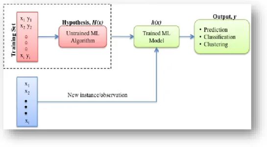
algorithm (Abu-Mostafa et al., 2012). Furthermore, the input data may be separated into a training and validation set. Figure 1 provides a generalized depiction of machine learning along with some of the terms that are commonly used in this section.
Figure 1 Generalized Depiction of Machine Learning
As the name implies, the training set is use to select the optimum hypothesis h(x), from the space of hypothesis, H(x). Succinctly, training data is used to build a model that can used to predict, cluster, or classify new instances. The hypothesis is in fact a function that maps the input vector X to an output Y; written formally, 𝐹: 𝑋 → 𝑌. The function,
h(x), is representative of the particular ML algorithm used. In Figure 1 the input data has a single feature, x; however, in practice the input feature space may be very large, as in the case of classifying photos of common objects where a single picture may have 256x256 pixels. Selection of a particular ML algorithm, e.g. linear regression, logistic
regression, perceptron, etc. is a function of the data, task, and the preference of the analyst.
Finally, the validation data set is use to evaluate the trained ML algorithm, h(x). A well accepted method for evaluating the quality of a ML model is to measure recall and precision. Recall and precision are defined as follows:
Recall represents the proportion of all the instances of a particular class that are correctly classified as that class (Blair & Maron, 1985; Flach, 2012; Hand, 2009). Concisely, did the classifier correctly classify all the instances of a particular class. To calculate recall the following expression is used:
𝑅𝑒𝑐𝑎𝑙𝑙 = 𝑇𝑟𝑢𝑒 𝑃𝑜𝑠𝑖𝑡𝑖𝑣𝑒𝑠
𝑇𝑟𝑢𝑒 𝑃𝑜𝑠𝑖𝑡𝑖𝑣𝑒𝑠 + 𝐹𝑎𝑙𝑠𝑒 𝑁𝑒𝑔𝑎𝑡𝑖𝑣𝑒𝑠
Precision represents the proportion of instances that were classified as a particular class that are actually classified correctly (Blair & Maron, 1985; Flach, 2012; Hand, 2009). In short, out of the instances classified, what percentage of them are correct. Precision is calculated using the following expression:
𝑃𝑟𝑒𝑐𝑖𝑠𝑖𝑜𝑛 = 𝑇𝑟𝑢𝑒 𝑃𝑜𝑠𝑖𝑡𝑖𝑣𝑒𝑠
𝑇𝑟𝑢𝑒 𝑃𝑜𝑠𝑖𝑡𝑖𝑣𝑒𝑠 + 𝐹𝑎𝑙𝑠𝑒 𝑃𝑜𝑠𝑖𝑡𝑖𝑣𝑒𝑠
Both recall and precision are important for assessing classifier performance. If a classifier has high precision – indicating that the majority of observations classified were classified correctly – and the classifier failed to classify many of the target instances (i.e., poor recall), then the overall performance cannot be considered good. The converse is also true, where recall is high and precision is low. In the following section the three ML
algorithms used in this research, SVM, Naïve Bayes, and C4.5, is described in more detail.
Support Vector Machine
Support Vector Machine (SVM) has become one of the most popular supervised ML algorithms and is applied to a wide range of tasks within the field of genetics, medical science, security, and network analysis (Burges, 1998). Although SVM is based on a linear classification model, its ability to be extended to tasks with high dimensional features, with a relatively small training set, has only widened its use across a variety of problem sets (Burges, 1998; Yuan et al., 2010). Moreover, SVM can be applied to binary, multi-class, and non-linear classification problems, while still maintaining a high degree of efficiency (Chang & Lin, 2011; Chih-Wei & Chih-Jen, 2002).
SVM is considered a large margin classifier since it constructs a hyperplane (decision boundary) that offers the greatest separation between the different classes of data under analysis (Muller, Mika, Ratsch, Tsuda, & Scholkopf, 2001; Tsochantaridis, Joachims, Hofmann, Altun, & Singer, 2005). Since the hyperplane has a large margin between positive and negative classes, SVM mitigates issues associated with
misclassification of new unlabeled data instances; succinctly, the trained classifier is more generalizable to new instances of the data than a basic linear classification model (Smola & Schölkopf, 2004). In the following sub-section, a discussion of SVM, along with an overview of its mathematical underpinnings, is detailed initially from the
perspective of a generic linear classification task, followed by an overview of a nonlinear case.
Linear SVM (LSVM)
LSVM is the most basic SVM model that supports binary classification of data into negative and positive classes, assuming the input data is linearly separable. For example, given a data set D defined by the following
𝐷 = {(𝑥𝑖, 𝑦𝑖) | 𝒙 ∈ ℝ𝑑, 𝑦 ∈ {1, −1}}, 𝑖 = 1 … 𝓃, (1)
where the vector 𝒙 represents a set of scalar data points 𝑥1… 𝑥𝑛 that can be used to train and test a function that maps the input data to the output 𝑦. The dependent variable 𝑦 will be either 1 or -1 for positive and negative classes, respectively. Since SVM is a
supervised learning algorithm, all training data instances were labeled with either a 1 or -1 when training the classifier. Furthermore, given this is a linear classification task, the SVM function to be trained with dataset D can be described by the following expression
𝑦 = ℎ(𝑥) = 𝒘 ⋅ 𝒙 + 𝑏; 𝑦 ∈ {1, −1} (2) where 𝒘 is the normal vector to the decision plane, 𝒙 is the input vector, and b is the bias
or offset. Additionally, equation 2 specifies the dot product of vector 𝒘 and 𝒙 which is defined as
𝒘 ⋅ 𝒙 = ∑ 𝑤𝑖
𝑛
𝑖=1
𝑥𝑖 (3)
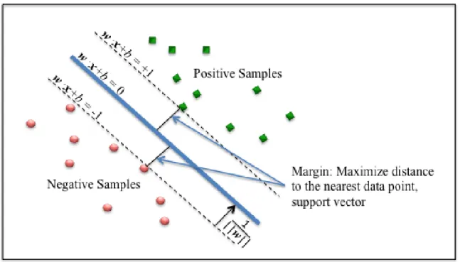
To gain better intuition of the details regarding SVM, Figure 2, based on Flach (2012), is used as a reference for a generalized LSVM and the discussion that follows.
Figure 2 Linear Support Vector Machine
As depicted in Figure 2, the decision boundary hyperplane, is specified by
𝒘 ⋅ 𝒙 + 𝑏 = 0 (4) and the maximum margin hyperplanes are defined by
𝒘 ⋅ 𝒙 + b = 1 𝒂𝒏𝒅 𝒘 ⋅ 𝒙 + 𝑏 = −1 (5)
separating positive and negative values, respectively. Constructing the maximum margin hyperplanes (dashed lines) for both positive and negative classes is based on the data instances nearest to the decision boundary hyperplane, which are referred to as support vectors. The Euclidean distance from the maximum margin hyperplanes defined by equation (5) to the decision boundary hyperplane, equation (4), can be determined using the following 1/|(|𝒘|)|, where ||w|| is the norm of the vector 𝒘. Intuitively, minimizing
||w|| will maximize the distance between the nearest positive or negative sample to the
decision boundary hyperplanes, which implies the following constraint optimization problem.
min 1
2∥ 𝑤 ∥
2 subject to 𝑦
𝑖(𝒘 ⋅ 𝒙 + 𝑏) ≥ 1, ∀ 𝑖, 𝑖 ∈ {1 … 𝑛} (6)
Extending LSVM
Two key limitations arise from the constraint optimization problem expressed in (6), its ability to deal with input data that is not linearly separable (non-linear feature space), as well as a high dimensional input vector space (Flach, 2012). In order to addresses these issues, the introduction of a soft margin constraint, Lagrange multiplier, and a Kernel function will be explored (Flach, 2012).
First, the addition of slack variables to the objective function and constraint in equation (6) will relax the constraint and introduce the concept of a soft margin (Tsochantaridis et al., 2005). The addition of slack variables allows some degree of misclassification, which assumes that the data may not perfectly satisfy the linear constraint that was imposed in equation (6). Concretely, if the input data is noisy or not linearly separable, then the constraint 𝑦𝑖(𝒘 ⋅ 𝒙 + 𝑏) ≥ 1 will not be met. By applying a slack variable 𝜉 to the constraint, some degree of margin violation is allowed, which begins the process of addressing non-linearly separable data (Tsochantaridis et al., 2005). Accordingly, slack variables are added to both the objective function and the constraint for the SVM. Moreover, a penalization parameter 𝐶 is introduced to balance the effects of slack variables on the objective function. Therefore, equation (6) takes the form
min 1 2∥ 𝒘 ∥ 2 + 𝐶 ∑ 𝜉 𝑖 𝑛 𝑖=1 subject to 𝑦𝑖(𝒘 ⋅ 𝒙 + 𝑏) ≥ 1 − 𝜉𝑖 𝑎𝑛𝑑 𝜉𝑖 ≥ 0 ∀ 𝑖, 𝑖 ∈ {1 … 𝑛} (7) where the parameter C is used to minimize the effects of the sum of the slack variable 𝜉 on the objective function.
By convention, a linear optimization problem of the form specified in (7) can be approached using Lagrange multiplier 𝛼 to find the extrema of the objective function under the specified constraint (Cortes & Vapnik, 1995). Furthermore, by devising the dual form of the Lagrange function the SVM optimization problem, equation (7) can be expressed as follows, max ∑ 𝛼𝑖 𝑛 𝑖=1 − 1 2∑ ∑ 𝛼𝑖𝛼𝑗𝑦𝑖𝑦𝑗 𝑛 𝑗=1 𝑛 𝑖=1 (𝒙𝒊⋅ 𝒙𝒋) subject to ∑𝑛𝑖=1𝛼𝑖𝑦𝑖 and 0 ≤ 𝛼𝑖 ≤ 𝐶, 𝑖 ∈ {1 … 𝑛} (8)
Completing the process of making SVM applicable to non-linear problem sets requires the addition of Kernel methods to equation (8). Kernel methods are functions that can be applied to various ML algorithms to address non-linearity of input data and has proven to be well suited for SVM (Burges, 1998; Cortes & Vapnik, 1995; Howley & Madden, 2005). By replacing the dot product in the optimization in (8) with a Kernel function, the equation takes the form
max ∑ 𝛼𝑖 𝑛 𝑖=1 − 1 2∑ ∑ 𝛼𝑖𝛼𝑗𝑦𝑖𝑦𝑗 𝑛 𝑗=1 𝑛 𝑖=1 𝐾(𝒙𝒊⋅ 𝒙𝒋) subject to ∑𝑛𝑖=1𝛼𝑖𝑦𝑖 and 0 ≤ 𝛼𝑖 ≤ 𝐶, 𝑖 ∈ {1 … 𝑛} (9) where 𝐾(𝒙𝒊⋅ 𝒙𝒋) represents the application of a Kernel function to the SVM (Flach, 2012). This approach allows the algorithm to fit a non-linear input data set to a large margin hyperplane decision boundary in a high dimensional feature space. There are several Kernel functions that can be used to support this transformation; although, Gaussian Kernel is one of the more common methods used across a large spectrum of problem sets (Chang & Lin, 2011; Keerthi & Lin, 2003).
Finally, as stated previously, SVM can be applied to multi-class problem sets. For multi-class systems, the most rudimentary method used is the principle of one-against-all, whereby multiple SVM algorithms are independently trained to identify a particular class of the data, say red, blue or green, and then applied against new instances (Weston & Watkins, 1998). As expected, each classifier identifies the input data it was trained on for a given instance, providing the effect of a multi-class classifier system.
Naïve Bayes
In general, probabilistic ML algorithms can be characterized as either discriminative or generative. Discriminative algorithms estimate the direct posterior probability between the input vector X, and a target class Y, 𝑃(𝑌|𝑋), without any understanding of the
underlying probability distributions that may exist (Ng & Jordan, 2002). Generative algorithms model the joint conditional probability distribution between the target class Y
and the input vector X, succinctly 𝑃(𝑋, 𝑌), accounting for the underlying probabilities, likelihood, and prior probability of the target class (Ng & Jordan, 2002). Although Naïve Bayes ML algorithms are comparatively less complex than other supervised learning models, it has been empirically proven to be effective across a variety of problem sets (Soria, Garibaldi, Ambrogi, Biganzoli, & Ellis, 2011).
From Bayes Rule to Naïve Bayes
Fundamentally, Naïve Bayes is simplified form of Bayes rule, with the inclusion of a key assumption that allows its practical application to ML tasks. Any discussion of Naïve Bayes, must begin with Bayes Rule, which is defined as
𝑃(𝑌|𝑋) =𝑃(𝑋|𝑌) 𝑃(𝑌)
where 𝑃(𝑌|𝑋) is the posterior joint conditional probability of class Y given the input X
and is computed using the product of 𝑃(𝑋|𝑌), termed the likelihood, and the prior probability for the class Y, 𝑃(𝑌) (Friedman, Geiger, & Goldszmidt, 1997; Lewis, 1998). The denominator, 𝑃(𝑋), is used to normalize the resulting posterior probability to a value less than or equal to 1.
To begin extending Bayes Rule to the Naïve Bayes algorithm, the focus is on maximizing 𝑃(𝑌|𝑋), as expressed by
𝐶𝑙𝑎𝑠𝑠 𝑜𝑓 𝑋 = 𝑚𝑎𝑥 𝑃(𝑌|𝑋) (11) or stated more explicitly,
Class of 𝑋 = max 𝑃(𝑋|𝑌) 𝑃(𝑌)
𝑃(𝑋) (12)
which indicates that the classification of X for a target class is a function of the largest joint posterior probability (Mitchell, 1997; Seeger, 2011). Understanding that X is a vector that is comprised of a set of features, 𝑥1… 𝑥𝑖, a key assumption can be introduced to simplify this formulation to reduce the complexity of calculating the likelihood when using data with a high dimensional feature space and a large number of samples.
Specifically, it can be proposed that the likelihood value 𝑃(𝑋|𝑌) can be expressed as the combination of individual and independent probabilities of each input feature with respect to a given class, i.e. 𝑃(𝑥1… 𝑥𝑖|𝑦𝑗=𝑡𝑎𝑟𝑔𝑒𝑡 𝑐𝑙𝑎𝑠𝑠). This postulation constitutes the “Naïve” assumption for Bayes Rule and is referred to as conditional independence (Koc, Mazzuchi, & Sarkani, 2012). Written generically,
𝑃(𝑥1… 𝑥𝑖|𝑦𝑗) = 𝑃(𝑥1|𝑦𝑗) ⋅ 𝑃(𝑥2|𝑦𝑗) … ⋅ 𝑃(𝑥𝑖|𝑦𝑗) (13)
represents the product of the independent conditional probabilities of x given a class y. This significantly simplifies the calculation of P(X|Y). Furthermore, the denominator for
the Bayes Rule, 𝑃(𝑋), can be dropped since its value is constant for the entire input dataset (Mitchell, 1997). Consequently, P(X) does not affect the resultant joint posterior probability and is in accord with the assumption that each feature is conditionally independent across the entire feature set and sample space. Thus, the final form of the equation for Naïve Bayes can be expressed as follows
𝐶𝑙𝑎𝑠𝑠 𝑜𝑓 𝑋 = max 𝑃(𝑌|𝑋) = 𝑃(𝑦𝑗) ∏ 𝑃(𝑥𝑖|𝑦𝑗) (14)
𝑛
𝑖=1
where the class of a new observation is the product of independent likelihoods, multiplied by the prior probability 𝑃(𝑦𝑗) for a specified class.
Estimating Probability Distributions for Naïve Bayes
Generating the required probability distributions for the Naïve Bayes classifier can be performed using maximum likelihood estimates (McCallum & Nigam, 1998). Concretely, the training set is used to estimate 𝑃(𝑋|𝑌) and 𝑃(𝑌) by examining relative frequencies for each class and attribute in the dataset. First, the probability of a class, 𝑦𝑗, within a given dataset can be estimated by the following
𝑃(𝑦𝑗) =|𝑦𝑗|
|𝐷| (15)
where |𝑦𝑗| is the number of occurrences of a specific class normalized against the total number of instances, |𝐷|; and to determine likelihood, the following formulation can be used
𝑃(𝑥𝑖|𝑦𝑗) = #𝑥𝑖 𝑓𝑜𝑟 𝑐𝑙𝑎𝑠𝑠 𝑦𝑗
where the numerator represents the frequency that the attribute 𝑥𝑖 occurs for the specified class, 𝑦𝑗, normalized by the count of all of attributes within the training set that have the class 𝑦𝑗 (McCallum & Nigam, 1998).
Since maximum likelihood is used to determine component probability distributions for Naïve Bayes, in real-world problems certain distributions of an instance’s feature may be equal to zero for a given class. Simply stated, the training set may not have an
occurrence of a particular attribute-class pair, while a new observation may in fact
represent such an attribute-class relationship. Based on equation (14), which specifies the class of a new instance is a product of independent probability distributions, a zero probability can in effect lead to an unknown classification – zero for P(Y|X). In order to address this issue, Laplace smoothing can be used (F. Peng, Schuurmans, & Wang, 2004). In its most basic form, Laplace smoothing can be implemented by adding one (add-one-smoothing) to both counts in equation (16) as follows:
𝑃(𝑥𝑖|𝑦𝑗) = #𝑥𝑖 𝑓𝑜𝑟 𝑐𝑙𝑎𝑠𝑠 𝑦𝑗+ 1
∑∀ 𝑣#𝑥 𝑓𝑜𝑟 𝑐𝑙𝑎𝑠𝑠 𝑦𝑗+ |𝐷| (17)
where the value |𝐷| is a more compact form for adding one to each occurrence of an attribute of class 𝑦𝑗. The result of add-one-smoothing is to ensure that missing attribute-class pairs in the training set do not impair the ability for the algorithm to attribute-classify new, unknown instances.
While the formulation of Naïve Bayes is based on a simplifying premise, it has exhibited excellent performance in terms of computation time and classification results despite the assumption of conditional independence (Rish, 2001; Yuguang & Lei, 2011). In fact, Naïve Bayes has become the de facto standard for text classification and
sentiment analysis where it is used in conjunction with ensemble techniques (Rennie, 2001).
C4.5
One of the more practical inductive machine learning methods are decision trees (Safavian & Landgrebe, 1991). A decision tree represents a classification task as a structure containing a root, branches, and leafs. The root of the tree, which itself is an attribute (feature), is the starting point of the structure, with each associated branch representing a decision point based on testing the value of an attribute, and each leaf equating to a specific classification of the input data under analysis. Decision tress can also be represented as a series on conditional statements (if-then), a sequence of rules that illustrates the testing of an attribute value to determine the final classification of an instance. Objectively, it is important to select the most appropriate root attribute and subsequent branch attributes to reduce decision tree complexity, computation time and overfitting (Quinlan, 1986). Quinlan (1986) and Quinlan (1993) developed two methods, ID3 (Iterative Dichotomiser 3) and C4.5, respectively, to optimize the building of a decision tree classifier.
ID3
Simplistically, a decision tree can be created based on randomly and continuously generating individual trees from sample data, with the hope of building an optimal
classifier that can be generalized to new instances. However, depending on the size of the training data in terms of the various classes and attributes, this approach can be time consuming to generate a viable decision tree. Moreover, the selected decision tree may in fact be one that is overly complex, as well as computationally expensive when used to classify new instances. ID3 is a top-down, greedy methodology for inducing an optimal decision tree with less computational overhead for both the generation of the tree and the classification of new observations. Considering ID3’s top-down approach, it is critical for the algorithm to select an attribute for the root of the tree that ultimately minimizes complexity (number of nodes and branches), yet is efficient at performing classifications of new observations. One means for determining the root and subsequent descendant branch nodes is to use a statistical based methodology referred to as information gain that measures the relative importance of an individual attribute for classification of an
instance (Mitchell, 1997; Quinlan, 1986). In order to calculate information gain, two values are needed: the entropy of the entire dataset and the normalized entropy after the dataset has been split using an attribute (Quinlan, 1993). Entropy, within the context of information theory, is a measure of the impurity or uncertainty of a given dataset (Mitchell, 1997). An examination of how the entropy of a data set is calculated is first described, followed by a discussion of the normalized entropy after segmenting the input data using a selected attribute.
Given a training data set, D, which has two distinct classes (positive and negative, denoted by P and N, respectively), the probability of positive and negative instances is calculated by the following
𝑝⊕= 𝑝̂
𝑝 + 𝑛 𝑎𝑛𝑑 𝑝⊝= 𝑛̂
𝑝 + 𝑛 (18)
where 𝑝 ̂ and 𝑛̂ represent the number of positive and negative instances within the dataset normalized over all instances in the dataset (Quinlan, 1986). Since a decision tree returns a single class for any instance evaluated, it can be considered as a message source for each class, P or N, contained in the dataset (Quinlan, 1986). Accordingly, principles related to information theory can be applied to determine the information needed to generate a message for P or N. Based on this precept, the probability equations in (18) can be used to evaluate the entropy of the system and is specified by the formula
𝐸𝑛𝑡𝑟𝑜𝑝𝑦(𝐷) = −𝑝⊕ log2𝑝⊕− 𝑝⊝log2𝑝⊝ (19)
where 𝑝⊕ and 𝑝⊝are the proportion of positive and negative instances of the dataset (Fayyad & Irani, 1992). Note that if the input space D only contains a single class, then equation (19) for the entropy of the system evaluates to 0. Units for the output of equation (19) are in bits and range from 0 to 1, indicating the amount of information required to generated a message related to the class of an instance. The restriction of the dataset to a boolean classification is done for simplicity, and is not indicative of a limitation for ID3 or C4.5. Input datasets may contain significantly more classes than two. As such, equation (19) can generalized to the following
𝐸𝑛𝑡𝑟𝑜𝑝𝑦(𝐷) = ∑ −𝑝𝑖log2𝑝𝑖
𝑐
𝑖=1
where c is the total number of distinct classes and 𝑝𝑖 represents the proportion of each class within the input space D.
Determining the entropy after splitting on an attribute follows a similar approach as the entropy for the entire dataset prior to dividing. However, the scope of the evaluation pertains to a single attribute and includes a normalization factor. More explicitly, if an attribute A with values {𝑎1… 𝑎𝑣} is used as the root of tree, it partitions the input space D
into a subset of branches and associated classes, using each attribute value. That is, for each attribute A, and its associated values 𝑎𝑣, a subset of the objective decision tree can be formed by testing the different values for A. Accordingly, the entropy for the sub-tree generated from this activity can be evaluated with respect to the particular attribute under test. Written formally,
𝐸𝑛𝑡𝑟𝑜𝑝𝑦(𝐴) = ∑𝑝̂𝑖 + 𝑛̂𝑖 𝑝 + 𝑛
𝑣
𝑖=1
𝐸𝑛𝑡𝑟𝑜𝑝𝑦(𝐷) (21)
where 𝑝̂𝑖 𝑎𝑛𝑑 𝑛̂𝑖 represent the number of positive and negative classes related to the attribute 𝐴𝑖 being evaluated, normalized by the total number of positive and negative instances for the entire input data space D.
Now that both the entropy for the entire input data set D and the normalized entropy for each attribute can be determined, information gain can be used as a measure of the effectiveness of an individual attribute for classifying data. Stated differently, information gain for an attribute is a measure of the reduction of entropy for classifying the dataset when a particular attribute is used to partition the data (De Mántaras, 1991; Mitchell, 1997). Written formally