WORKING PAPERS
Debt and International Finance Ifnternational Economics DepartmentThe World Bank May 1990 WPS 408
Methodological Issues
in Evaluating
Debt-Reducing Deals
Stijn Claessens
and
Ishac Diwan
I lere is a
sinmpie
method bor identifying the best debt deals aCoLIntry can haruain tor
\
ith its creditors \hen debt reductionatnld new nimney are thei only (optionis availalhi. .4
"a.
I P!:e 1 , R. a7.' I V!. , I:(- :i'.' k I a Pi i-e' ;o- .d: t l: C c Endings of aork in prngncss
a ' d .' 2'' . ' .a¢s.'i .' . H. '
- .'.'n'.'
.a-,o:.. 2c* *p ' .t.> m I%.Ceppt car e.) thCOJ...* TOCLW l''
a'.,.'"4'se' 'T<ittC
A~~~~~~~~~~~~~~~~a~ a-~tenre
Public Disclosure Authorized
Public Disclosure Authorized
Public Disclosure Authorized
Polic.r, Research, and EAternal Affairs
* 5 5:1
Debt and International Finance
'I'his paper -a prodUCt 01 tle Ikbt anll l ncationajl Iinance IjrrivSji, Intejlionll L onlom icS
D)pljt_-IIrit -
i^
parl of a laIrgcer e tIort In PR kf 1tittller-cial F to s taud tie respon1cs crcdiors to difterinideht restrclturinu deals, >to as to d,>ie d lik hlciti arc l ore, la\orablc 10r the COUtrII . pIies:'
availabhle 1recl Irori Oic \World Bank, I 18 II Stirctl NW'. a'shistgtiltoni )C( 2433. Please contact Sltci' di
Kin-W'atson, roomn S -0255 extcnsion 3373,0 (1 37 pagCs w;ith graphs and tables r.
'F1ie
novel(r
c 111(t complexity of me'nu hased dcbh c * That (the nere existenlC o1f ;1 aLisCoLunIt on llthereductioln d]Cals unider the Brad .m Iniiiati\e make sccondar\ market is a sulficienit conlditioIn for
it diiflicult to see througcl thc smolke andl rn i roros bu\haacks that are proflitabIc lor a debtor.
of' financial engineering. Clacssenis arnd Dmi;an
explain thc esscntials. Drawing oti applications in Mexico, Costa
Rica, aridl tle lhtlilippines, Claessens and Diwan
ThCe Cxplalin the buil(dillg blocs for anal\/- present a simple nietthodi lor identifying the best
ing debt dcals, discuss comi mon pi taltlls. and in- dcebt dcals. in temis of dcebt rceductioni andl
trodluce thc corncept ol' iteC deht ValiUC Curv c. I(iL'idit\. a counltr can hargain lI'r vith its
T[hey anal vc in dctail lthC main instrurnieits creditors \heIn (dcbt reductionl and new.C monev available for debt reduction: bu\ hacks: an are thic options. 1Thev emphasize that tic pro;vi-exchlallng ot loreign debt againsnt another torciL n siori of nc mone\ is best v ic\ecd as a conices-alsset sittl w lilltd relirent tirms: and anl xc1ha1nee ol sioni h! nion-c\xisting creditors in cxclhange or foreigni decht against a (domestic asset (a dlch- tile ' alileC increazse of their existing dcht on
equit\ s5klf). Tlite delscribt hozs to puit tlie ac.count ol tlic debt reduction.
diifertent ccmntcs or u det.l t'ctlirit lo Atr ij\ .At
a suital1e badlanc. e ct). Cn. ecu t rc<ldi,iwu ond Nokm tire challcriro ik to idetllith etc deal that liquldit\. Anld tle\ c the iiW 11,:t of euoi is bcst tor tic thecoulllr\ (ri\en its pir-cerenccs
lcndcrs on deht dIals. rNl)ut hquldit\ \%er>SUS dehbt redICt6io1n andi La,t1.
I,ill cc pt ab'lI to its creditors, That \ ill
T'le\ crrphisi/t' \k o l>ci' in \wltimtil%r re,quire ai Leneral cquilibnruilm nacroecorrovrric
deht rdctl.40 t1or dil\ model tO ana\Iie' a cOulntr'S illxcstlert.
gr ox tir.an TL'repA\ it'S lblea. irla rA xlien1 tlir 'Iftll t oluillta riallkelt hb;t.u<cd mt.eclurr1collisuntrx har! s ai orci-.ri credit const:aiiint ard a debt airc akk A'\ S good lOr aill, The ai1\ Urlle'C 0Ill \ erhalg. It xxiii AlSo reLlul re a tter
under-Ilnarke t'l-ba;t'.cdl ncIlarrti\rli'xl ' tlr ihex ,ct S; ilKlill'di u oftox 1 aInkS 1make a1 choice \A hen
airouLndi cOIlleCixC eCact ion pr4!lcrrl but tl:x r''u tc \ xilh
.i
illr oh optiorlodont tieco,-arr lx bnfict'i oxe\ orekk.
\f fai r I CO ''I 0.' T 1 I' I I I . ' ' ! ' " : thX1 !i.!!.
DEBT - REDUCING DEALS
Eoreword
This paper is motivated by the rise in market-based debt reduction schemes a,.d the official support for debt reduction as in the Brady plan. Both developments require a better understanding of the different types of debt reduction schemes, their essential characteristics and their benefits and costs. The paper is especially motivated by the development of concerted debt reduction schemes that combine debt reduction with new money.
The paper builds on earlier work in the division and bridges the gap between earlier analyses of concerted new money deals and market-based debt reduction techniques. Applications of the analysis to recent debt restructuring deals demonstrate the relevance of the issues analyzed.
2
METHODOLOGICAL ISSUES IN EVALUATING
DEBT - REDUCING DEALS
by STIJN CLAESSENS AND ISHAC DIWAN Table of Contents Page I. Introduction ... 3
II. Building Blocks .. 3
1. Instruments ... 5
2. Pitfalls and Fallacies of Market Based Debt Reduction Deals ... 6
3. Status-Quo and the Diverse Interest of Banks ... 7
4. The Debt Value Curve ... 8
5. Involuntary Lending ... 11
III. Analysis of the Elements of a Menu . . 12
1. Buybacks ... 12
2. Senior Exit Bonds ... 15
3. Debt Exchanges and Collateralization ... 17
IV. Characterizing the Best Debt and Debt Service Reduction Deals . . . 21
1. Dilution Mechanism ... 21
2. Debt Deals that Maximize the Return on Official Loans: the Debt Reduction-Liquidity Frontier ... 23
3. Preferences over Debt Reduction and Liquidity ... 23
4. Other Dimensions of the Deal ... 26
5. Applications ... 28
5.1 The Recent Mexico Deal ... 28
5 2 The Philippines ... 31
5.3 Costa Rica ... 32
6. Seniority, Prices and Buybacks ... 34
V. Conclusions ... 35
METHODOLOCICAL IS!'IES IN EVALUATING DEBT - REDUCING DEALS
I. Introduction
The Brady Initiative has intcoduced official support for debt reduction. This new phase in the debt strategy requires a new set of tools to analyze debt
deals and to study the impact of a deal on the debtor country. Since debt
reduction as well as new money instruments are now negotiated simultaneously in a partially concerted environment, the kind of analysis will have to be different from that used in the market-based menu approach, where debt reduction
instruments were negotiated with banks individually.
This paper discusses first the methodological issues involved in evaluating the different individual components of a debt deal, i.e. in a market-based context, and shows that the evaluation can be reduced to a tradeoff in two dimensions: debt reduction versus liquidity. The paper presents next a specific model to evaluate a debt deal consisting of multiple components, i.e., new money and debt reduction instruments. The paper argues that creditors not participating in any debt reduction free-ride on the increase in value of the remaining debt. As a result, the debtor should be able to use debt reductions as a bargaining chip to extract some concessions from these non-participating banks. This leads to the important result that agreements more favorable to the country can be reached when a deal, including new money and debt reduction, is negotiated in a concerted environment, even when debt reduction remains market-based.
The structure of the paper is as follows. Section II presents the building blocks for an analysis of debt deals, discusses some common pitfalls, and introduces the concept of the debt value curve. Section III analyzes in detail the different instruments available for debt reduction: buybacks, senior exit
bonds and debt exchanges. Section IV puts the different elements of a deal
together and derives a debt reduction-liquiditv frontier. This section also applies the methodology to three recent debt deals: Mexico, Philippines and Costa Rica, and discusses the impact of senior lenders, such as the international
financial institutions, on debt deals. Section V concludes.
II. Building Blocks
The novelty and complexity of menu based debt deals makes it difficult to see behind the smoke and mirrors of financial engineering. This paper will simplify the analvsis by capturing the essentials behind menu driven deals under the Brady Initiative. (For the essential features of the Brady initiative we refer to the box).
4
The Brady Initiative
The main features of the Brady Initiative are the following. Debtor
countries are expected to maintain (or adopt) growth- and reform-oriented adjustment programs. In addit.on, they should take measures to encourage repatriation of flight capital and foreign direct investment. The IMF, World Bank and other official creditors will provide financial support for debt and debt-service reduction. The debt and debt-service reduction can occur through debt buybacks, exchanges of old debt at a discount for new
(partly) col.lateralized bonds, and exchanges of old debt for new bonds at
par value, with reduced interest rates. The international financial
institutions will not act as a party to the negotiations ber.ween the
country and its creditors. (Intervention by creditor goverT7n"p-ts is possible).
Over a three-year period, the IMF and the World Bank expect wo provide between $20 billion and $25 billion. Japan is envisaged to provide about $10 billion over the next several years (through cofinancing) as additional support. Commercial banks will provide debt reduction and new money, and support the accelerated :eduction of debt and debt service. Creditor governments will continue to reschedule official loans through the Paris Club and maintain export credit cover for countries with sound reform programs. Tax, account ng, and regulatory impediments to debt reduction in creditor countr; s will be eliminated.
The barebones of any menu driven debt deal consist of: a new money instrument;
an enhanced debt reduction instrument (buvback or exchange);
loans from international financial institutions (IFIs) that are
dedicated to debt reduction.
This barebones setup allows us to derive some lessons which are crucial
and to characterize what type of deal is best for a debtor. A two step procedure
is usel.
(i) First, we look for the set of feasible deals which offer the creditors a
net payoff equal to the status quo in terms of expected net present value. For this, it is necessary to identify the status quo against which the creditors and the country compare any debt deal. This also requires an understanding of how banks evaluate different claims, in particular, new money calls and exit bonds.
(ii) Second, we specify the objective of the country in terms of two parameters: debt reduction--a reduction in the present value of future obligations--and new liquidity to be used domesticall1 for investment or consumption
deals amounts then to the rip't trade-off between debt reduction and new liquidity.
Before being able to identify the right tradeoff, we need to develop some tools. We will describe first the basic instruments of a menu driven deal, discuss some common misconceptions, analyze the pricing of debt--in order to evaluate which type of deals would be acceptable to banks compared to the perceived status quo payoffs--and analyze involuntary lending.
1. Instruments
Market based debt and debt service reducing transactions can be divided into three broad categories: buybacks; exchange of foreign debt against another foreign asset with different terms; and exchange of foreign debt against domestic asset (debt-equity swaps). The instruments are described in detail in the box.
2. Pitfalls and Fallacies of Market Based Debt Reduction Deals
It is useful to dispel first some common misperceptions and fallacies regarding market based debt deals. We will concentrate on two.
A first c-nmmon fallacy is that voluntary market based mechanisms are always
good for all. While it is true that market based mechanisms by definition get around collective action problems, and may therefore te advantageous, they do not necessarily benefit all. A zimple example of how a market based mechanism may backfire would be the following.' Suppose a country owes a large sun to its creditors and has an investment opportunity which, from creditors' point of riew, is very profitable as it yields much more than their cost of funds, however, less than the total amount the country owes them. Suppose also that the country has some excess reserves at hand (or has access to a loan from the IFIs), which it
can use for either the investment project or for a buyback. Now suppose the
country spends its reserves buying back its debt on the secondary market. If the country succeeded in buying back debt, it would make creditors worse off: to get
the reserves, they need to give up a profitable investment opportunity. The
country would also be worse off, since it would have spent all current resources (or would have reduced current consumption) without receiving any future investment income.
Such a scheme would clearly be very foolish. A concerted agreement is unlikely to lead to such a scheme. The irony is, however, that this scheme could
be supported by the creditors under a market-based menu. The logic is that each
creditor would reason, given that other creditors are redeeming their claims (and therefore the investment project has effectively been cancelled), that his claim would be worthless if he tried to hold onto them. On the other hand, if he
redeemed his debt, he would at least receive some cash. Thus, each creditor
would reach similar conclusions abou. their prospects and be willing to
tClaessens and Diwan (1989) mention this point. See also Claessens, Diwan,
6
Debt Reduction Instruments. Description
Buybscks: In this type of transaction, a country (Bolivia and Chile are examples) buys back its debt at a discount in exchange for a cash payment. But countries with debt servicing difficulties rarely have much ready cash, and therefore the Brady initiative envisions external support. In case of Bolivia and Chile, there were exceptional circumstances that facilitated the debt buybacks (the Bolivian operation was financed by aid agencies and Chile had excess reserves because of unanticipated increases in the price of copper).
Exchange of claims: An exchange of old debt for a debt instrument with lower principal or interest. In order for the exchange to be voluntary, the new instrument must be a more secure asset in the eyes of the
creditor. Three
~actors
can make new instrument more secure. First, thebanks can collec:ively agree that exit bonds have seniority over other claims. This, however, is unlikely to occur. Second, the IFIs could guarantee them. Third, the new asset can be backed by collateral for the principal or for interest payments, or it can have special conversion
rights. In addition, thLe new instrument can be more valuable to the
creditors because of certain tax, regulatory and accounting advantages. To purchase the collateral, the country can use it own resources cr obtain (part of) the resources from ocher sources--such as the IMF and the World Bank.
Debt Eguity swaps:Debl:-equity swaps. An investor exchanges a foreign loan
for local currency to be used for domestic investments. If the debt retired is public debt, the government effectively prepays debt in domestic currency, sometimes at a discount. Wh( private sector debt is retired (at a discount), the government loses (1, terms of cash flow) as the debt service would have been paid to the central bank by the private sector otherwise for later payment to external creditors.
participate in a buyback. Of course, if the debtor would stand to gain from investing (e.g., the return on the project exceeds the contractual obligation
to its creditors), it would not be in its interest to initiate a debt buyback.2
This demonstrates that market-based schemes may solve one collective action problem but do not lead to an optimal situation. Letting individual creditors choose what is best, without any collective guidance as to which alternatives
2
1n the context of the Brady initiative this question amounts to whether the IFIs should restrict (additional) funds to be used for debt reduction transactions alone or allow them to be used for investment also. If the IFIs restrict the additional funds to be used for debt reduction both the debtor and the creditors could agree to a debt reduction scheme even if there exist profitable investment opportunities in the country.
are admissable, can lead to Pareto-inferior outcomes. In the sequel, we will analyze schemes that consists of a menu of admissible options which are (to a
large extent) agreed upon between the country and the creditors collectively. The design of the overall scheme is a concerted effort, but each individual creditor is free to choose among the options. At the same time the scheme has to be in the interest of the debtor.
A precondition for a successful menu deal is that some mechanism is in place to guarantee that al'. creditors choose one of the options. Free riding--collecting payments without contributing new money or engaging in debt
reduction--has to be prevented.3 If free riding is prevented, a sharing of debt
relief by all creditors can t.ake place while the flexibility to accommodate
differences between creditors is preserved.
The second fallacy of voluntary debt reductions is that the mere existence of a discount on the secondary market is a sufficient condition ior buybacks which are profitable for a debcor. This view is based on the notion that, since countries will need to repay their debts in full if they return to prosperity, they are better off retiring debt when it is cheap. Such reasoning is flawed however since it does not take into account the very real possibility that debtors don't return to prosperity--which is exactly the re&son for the discount The Brady Initiative has shown a reluctance on the part of creditor governments to commit large sums of public money to buy back debt even though secondary market prices are significantly below par. This is a further indication that a discount is not a sufficient condition for profitable buybacks. In the absence of a clear indication of either an upward or downward bias in secondary market prices, we conjecture that they represent a fair estimate of the expected value per unit of debt, in which case buybacks are not necessarily beneficial for the debtor.
3. Status-Quo and the Diverse Interests of Banks
Even though a menu approach allows for differences among banks, the determination of the elements of a menu, their relative pricing, and the sources of the funds used to finance debt reduction remain matters that can divide banks. Divergence--between banks that want to exit and that want to stick to the new
money approach- -imposes restrictions, since under the syndicated loan agreements
each bank is iil a position to veto contract changes. Each bank must therefore
perceive that it is equally well off compared to the alternative situation, call it the status-quo. Other parties involved, the IFIs and the debtor country, must also perceive that the new deal offers them at least as much as the status-quo.'
3
Free-riding can be limited in several ways: i) through legal mechanisms (so-called novation, see the discussion of the 1989 Mexico deal, section IV.5); and ii) through coercion mechanisms applied by the IFIs (such as condoning arrears to creditors not participating in the deal) and the creditor governments.
4Expectations of future deals will of course also matter. We assume that
the deals being analyzed are the only ones expected for the foreseeable future, or that they represent the sum of the future deals that are expected to take place. Similar for the specified al.ernative.
P
The constraints that follow from this are:
* No individual bank should perceive that it loses compared to its
status quc. Otlherwise, the bank could veto the deal. This implies:
* Existing banks must receive at least--in present value
equivalents--the value of their >'aims in the status quo.
* Remaining banks providing new money payoffs must receive a
payoff no lower than the status quo. The gains from the
increase in secondary mnarket price (the result ot the debt
reduction) must exceed (or be equal to) the capital loss implied by the provision of new money.
* The IFIs must accept to fund (parts of) the debt reduction.
These constraints are not easily satisfied. Conflicts of interest are likely to arise between exiting and remaining banks. Take the case where debt
reduction is financed by resources that were available for de'-t service. A bank
will benefit by exiting if the price at which it sells its claims is higher than the perceived value of staying in. However, if debt is reduced the benefits of staying in and the price at which a bank will want to exit will be higher--due
to improved creditworthines. But the higher the exit price, the less debt
reduction there will be, and the less attractive the deal will be for the remaining banks. Thus, banks that exit must do so at a price which is considered a bargain by the remaining banks.5 In case the IFIs finance the debt reduction, then they must perceive that the debt reduction leads to an i.nprovement in creditworthiness of the country, which enhances the value of their claims, and contributes to some of their other objectives (such as stability in the country). Alternatively, consider the case where the funds for debt reduction would otherwise not have been available, e.g. foregone domestic absorption or the new external sources of the IFIs. In this case banks can exit at prices above their status quo price while still allowing for gains for the remaining banks, But
in this case, part of the benefits of debt reduction has leaked to thne remaining
lenders. The debtor and the IFIs migh refuse to participate in such a deal. In such cases a mechanism is needed tha- allows the debtor country to internalize most (or all) of the gains which are due to the reduction in debt, while at the same time making no commercial banks worse off. The mechanism is to for the cc.ntry to request from the remaining lenders current liquiditv in the form of new money loans.
4. The Debt Value Function
The analysis of debt deals, requires a further understanding of how the
5This can be the case when some banks are more pessimistic than others
about the future prospects of the country; when selling their claims, some banks enjoy larger tax advantages than others; and when some banks' costs of monito-ing their portfolios are too high given their small exposure.
secondary market evaluates developing country debt. Conceptual models as well as empirical observations support the view--holding everything else
constant--tthat the market value of debt ,alls short of its face value at an
increasing rate as indebtedness increases. This implies a decrease in the unit price of debt as indebtness increases.
Several empirical studies have measured t'.e relationship between prices
and face value of debt by estimating price equations (Claessens (1988), Purcell
and Orlanski (1988), Sachs and Huizinga (1988), and Vatrnick (1988)). Some of
these papers use regressions of the log of price on the log of debt and other
_onditioning variables in the form:
ln(pit) - a - 9ln(D),t + IYt + fit (1)
where pit is the secondary market price 0, is the total debt stock and Y,t is
a set of other regressors (such as measures of exports, arrears and
rescheduling), all for the ith country ,n vear t. The value of debt i.s given by
V - p*D - cD'-, where c is a constant related to a and Y in (1). The coefficient
R provides the elasticity of price with respect to the nominal value of debt.
Typically, estimates of 1 are in the range .3<R<.7.
The specification in (1) is problematic because it forces the elasticity to be the same at all levels of D. A better functional form for estimation is the logistic form:
ln(pjt/(l-pit)) - a - 9ln(D),, +yYYt +E.,,, (2)
with the elasticity of price not restricted to be the same across countries. Assuming that random noise separates the market price of two countries with an equal debt burden, (2) can be interpreted as an estimate of the average debt value curve across developing countries. The elasticity of price with
respect to debt is now a function of D and given by; [c9D'-l'/[l+cDBJ. Cohen
(1989) obtains an estimate for B of 1.2 for a set of 16 highly indebted
countries. Recent work by Claessens, Diwan, Froot and Krugman (1989, CDFK) finds
B-1.41 (and a-7.88) for a set of 35 countries.
The price equation used in the text is:
CDFK: ln [p/(l - p)] - 7.88 - 1.41*ln(D/X) (3)
where X stands for exports (Data set. cross sec in with 35 countries). 6
6
0ther equations which have been used and which lead to similar results
are: Cohen: ln [p/(l-p)] - 2.152 - 1.509*ln(D/X) - 0.048*Xgrowth
-0.583*Dummy(87.12) Data set: pooled equation, annual 1986 and 1987 for the Baker
17 debtors.
Salomon Brothers: ln(p) - 3.57 - 0.34*lnNDX + 0.23*InPCI + 0.78*RP + 0.47*Sl
+ 0.16*DE, where X is exports, PCI is per capifa income, NDX is debt net of
reserves over exports, RP - 0 if debt has been rescheduled, SI - 1 if interest
1.0
The debt value function associated with the CDFK price equation is drawn
in figure 1, with the market value v on the vertical axis and the size of the niomir.al debt D on the horizontal axis (both axis are scaled by the value of exports). The value of debt is a concave function of outstanding debt. For a given change in nominal claims, the associated change in the value of deb- is always smaller (as long as we.are on the,upward sloping side of the debt value curve).
o@t vadj !rsy.Ue
170 - -" 14 > 12P . 4 ,>, 30 -4 30H
/°t
30 100 2^0 330 4' 50G 6X' 70CApplication To Hypothetical Country
The secondary market price for an individual country will, apart from the level of debt relative to exports, be driven by many country specific factors. To apply the concept of a debt value curve to a specific country a price equation including more country specific variables would need to be estimated. The. price equa:ion listed above would likely not be sufficient. However, for analytical and illustrative purposes the estimated price equation can suffice as it captures
voluntarily trade an average claim for the marginal value of debt, because it
does not want to pay for Le relative improvement in the value of the claims of those that do not exit.
The fact that a market based buyback increases banks' payoff above that in the initial status quo and all the gains are internalized bv the debtor country suggests that a market-based buyback is best viewed as a concession to creditors. However, the fact that the debtor is not able to internalize all the benefits of a buyback does not imply that the transaction overall hurts him (or benefits him): it only implies that there might exist mechanisms that would allow for larger gains (or smaller losses). A non-market based deal where a buyback is combined with concessions from the creditors--in particular, with the
provision of new noney- -could be acceptable to both the creditors and the debtor.
The cr.^ditors group as a whole would receive the marginal reduction in market
value (AV) for t. reduction in debt (AD), the group's payoff would remain the same
as in the status quo, and the debtor would internalize more of the benefits of the buyback.
2. Senior Exit Bonds
Suppose that the country car issue and sell off a new set of securities called "secured exit bond", in return for outstanding bank debt: a debt exchange. The critical feature of such a debt exchange is that the new securities be accepted by the market as "senior" to original bank debt. By seniority, it is meant that the exit bonds will be paid before the remaining claimants. Seniority is critical in order for a debt swap to result in net debt reduction. Consider what would happen if the new bonds were expected to be treated in the same way as old debt. Then, the new bonds would sell at the same price as old debt and an exchange would result in no debt reduction.
There are some practical problems in creating senior debt. In this section, however, we will assume that it is possible to establish credibly the seniority of a new debt instrument which can be exchanged for existing debt. We will use a simple indicative example to see how such a debt swap works.
Imagine that the country's $100 billion total external debt belongs to the an identical "seniority class". Assume also that the country will with certainty make payments in the future whose present value is $42 billion. The implied secondary market price will thus be 42 cents. The country introduces now an exit bond with a face value of $1. We assume that the new bonds are
expected to serviced in full first, i.e. the new securit-y is senior and will be
valued at a price of 1. Because the market values each dollar of original debt
at 42 cents, 1 unit face value of new bond can be swapped for i/(.42) - 2.38
units face vallue of original debt.12
'2By conducting the analvsis for a small swap, we can ignore the fact that
debt reduction will increase the ex-post price and that therefore, the rmarket would value old debt given debt reduction at more than the original 42 cents. In the case of large swaps, less thon 2.38 units of old debt would be retired,
16
What is the gain from such a swap? The country has issued some new debt, but has retired a amount of old debt which is greater, without using cash. The net debt reduction is (about) $1.38. What happens to total expected repayments? In this case nothing, because the country made with certainty payments equal to $42 billion, less than its obligations. The debt-for-senior-debt swap would only have lowered the price of existing debt, since the new claim degrades the quality of original debt. But imagine, that there was a (very) small probability that the country had more than enough resources to pay the debt in full. In such circumstances, the debt reduction would benefit the country as the face value of debt, and thus debt payments, would have been reduced. The country would then have reduced its expected debt repayment through offering a one dollar of senior bonds, without using any current resources.
However, the scheme expiopriates the remaining creditors, which would not approve it. Syndication loan agreements explicitly include negative pledge clauses that prohibit the sale of more senior claims. Unanimous (or near unanimous) waivers are necessary to make new bonds more senior. Existing creditors will therefore not give any waivers of negative pledge clauses if the swap is expected to hurt them.
But how can one then comprehend debt reduction schemes such as the Mexico-Morgan debt swap of 1988? We will argue that in the Mexico-Morgan debt swap, no seniority was created and since Mexico used a cash collateral, the deal was not much different from a simple debt buyback.
The 1987 Mexico Swap
In December 1987, Mexico invited its commercial bank creditors to exchange outstanding commercial bank claims against Mexico for new bonds in, what was to be, the first major debt swap since the onset of the crisis. The new bonds had a 20-year maturitv, with the principal, but not the interest, collateralized by U.S Treasury obligations purchased bv Mexico using its own foreign exchange
reserves. Mexi.co was prepared to issue up to $10 billion of the new instrument.
With a secondarv market price of roughlv 50 cents, Mexico hoped that $20 billion of old debt would be retired.
Of course, MYexico tried to convince the market that the new debt was
senior. While it was not able to obtain waivers in order to establish this de-jure, Mexican officials suggested that the new bonds would be given a de-facto seniority, In particular, they claimed that the new bonds would be exempted from anv future restructuring agreement, and that loans exchanged for these bonds
would be excluded from the base for anv future request for concerted lending. 13
From the results of the auction it became clear that the swap was considered by the bidders as a collection of two transactions described above: a (self-financed) buyback of principal plus a debt swap of interest payments. It turned out that the interest payments were not evaluated differently from
3We will see later (section IV) that these exemption claims have become common usage.
regular Mexican risks and were discounted at the same rate implicit in the
secondary market price.14 Evidently, the Mexicans failed to establish seniority for the new bonds, and their debt swap degenerated therefore into a domestically financed buyback with the amount of resources equal to the value of the collateral.
3. Debt exchanges and collateralization
The major lesson of the Mexican-Morgan swap is that it is difficult to establish seniority beyond that implied by the security of a collateral. We will argue here that, as a first approximation, all collateralization schemes are more or less equivalent and lead to the same amount (net present value) of debc reduction for a given amount of resources. We will then list the circumstances for which this may not be true.
Debt exchanges that are partially collateralized (principal or interest or both) can be decomposed into a buyback and an uncollateralized debt exchange. What matters to the creditors is the total current value of the collateral rather than how the collateral is allocated across principal or interest, i.e., how it is spread out over time. However, there are situations in which this does not
hold.
The equivalence of different collateralization schemes to the creditors can be expressed as:
Value (collateralized bond) - Value (collateral) +
Value (old debt evaluated at post deal prices). The creditors are interested in the total current value of the collateral that is backing each $1 face value of bonds. The larger the current value of the collateral, the larger is fraction of "implied" buyback in the exchange.
'Using the interest rate at that time, the value of the collateral was equal to 21.7 percent of the face value of the debt. The present value of the
contractual interest obligations was 94.32 percent. Since other,
non-collateralized Mexican debt was selling for 50 percent, the expected present
value of interest payments was 43.65 cents. The total value was thus 21.7 + 43.65
is 65.35 percent, implying that $1.31 of old debt would be exchanged for $1 of bonds (an exchange ratio of 1.31). A price above 65.35 percent would have indicated that the market accepted some of Mexico promises for seniority. Of course, if the new bonds were considered fully senior, they would have sold for a price of almost one dollar.
In exchange for the $3.665 billion in face value of debt which offer price exceeded Mexico's minimum acceptable price, $2.557 billion of the new bonds were issued, backed by $492 million in collateral. Taking account of the fact that the interest rate on the new bonds exceeded bv a small margin that on the exchanged bank debt, the transaction turned out to have reduced the present value of Mexican obligations by almost the same amount as would have been achieved by a straight buyback using an amount of reserves equal to the collateral cost.
18
The fact that cred'Itors are indifferent between various possible collateralization schemes involving the same total current value of collateral, does not imply that the country will be indifferent too between different schemes. For instance, if the country is more impatient that the creditors (i.e., its rate of time preference is higher than the foreign interest rate), or if the countrv has better investment opportunities (i.e., its marginal productivity of funds is higher than the world interest rate), then the country can have a preference for collateralization schemes that lead to a higher reduction in debt service early on.15
The "implied" buyback equivalence proposition is easily illustrated in terms of a constant probability of default model. Consider a creditor holding $1 of debt with a risky interest pavment r for T periods and a sure $1 repayment at maturity. Assume that in each year, the debtor is expected to default on the risky debt--and pay nothing--with a probability (1 - 7). Assuming a risk neutral market, this claim would be valued at:
T
p - Value (Debt) - 2 rn/[(l+r)tl + [l/(l+r)T] (7)
t-l
Now consider a new bond BI which interest payments of $r in all periods, with the I first payments secured by a collateral (zero-coupon) and the remaining
(T-I) repayments unsecured. This claim will be valued at:
I T
Value(B,) - Z r/(l+r), + E rn/[(l+r),] + [l/(l+r)TI (8)
t-l t-I+l
The value of the risky debt and the bonds BI are not equal. The bond BI pa,-s a sure amount r in periods t - 1,2..I, while the risky debt pays in these periods with probability n. The bond will be more valuable than the risky debt and can be exchanged for a larger face value of risky debt. The exchange ratio between the debt claim and the BI bond, 61, can be defined as:15
6¾ - Value (Debt) / Value (B1) (9)
Two particular collateralization cases are of particular interest: (i) With no collateral (I - 0), Bo is identical to risky debt and
therefore So - 1.
(ii) With complete collateralization (I-T), Value(BT) - 1. As result,
6T - p, the price of the unsecured debt. Therefore, a complete
"5In fact, the debtor mav prefer to use the funds for immediate consumption or investment if that were allowed.
16We also define B as the share of collateral in the total value of a bond (see tables 3a and 3b). This concept will be used more in part IV.
collateralization is equivalent to a buyback.
Example of Collateralization
The probability of default at each period (1 - x) is 0.4. Take a
debt claim of $100 which matures in 30 years, where for simplicity, it is assumed that the principal repaid for sure in 30 years. Assume the debt
claim is swapped for a bond BI that has a coupon rate of 10% and on which
the first Ilh payments are secured through a collateral. The principal
$100 is also assumed to be repaid for sure in the 30th year. We compute
the cash price of BI, its exchange ratio and the present value of the needed collateral (table 3a). Note that full collateralization (I-30) is equivalent to a buyback. Under all collateralization schemes, the amount
of debt reduction per unit of collateral (netADj/V(C1)) is the same and
equal to that of a buyback. Cash flows involved may differ, but the present value of debt service reduction achieved will be the same.
Table 3a
Collateralizing the First I Payments
I - 0 1 2 5 10 20 30 V(F) 5.73 5.73 5.73 5.73 5.73 5.73 5.73 V(CI) 0.00 9.09 17.35 37.90 61.44 85.13 94.26 V(NCI) 37.70 34.0 30.76 22.54 13.12 3.65 0.00 V(BI) 43.43 48.89 53.85 66.18 80.30 94.51 100.00 SI 1.00 0.88 0.80 0.65 0.54 0.45 0.43 netAD, 0.00 12.56 23.97 52.36 84.87 117.59 130.21 netADI/V(C1)(%) 1.38 1.38 1.38 1.38 1.38 1.38 B 0.13 0.30 0.43 0.66 0.84 0.96 1.00 Notes:
V(F) is the present value of the terminal repayment.
V(Cj) is the present value of the I collateralized payments
V(NCI) is the expected present value of the (30-I) non-collateralized payments.
V(BI) is the cash price of a bond with I collateralized payments 6I is the exchange ratio, V(Bo)/V(BI)
netAD, is the percentage net debt reduction, (1/6, - 1)
netADI/V(CI) is the percentage net debt reduction per unit of collateral B is the share of the bond value derived from the collateral.
An example (in the box) shows that any collateralization scheme produces the same amount of net debt reduction per dollar of collateral. Collateralization of a bond does not lead to any leverage in terms of the amount of debt reduction achieved per unit of collateral compared to a buvback. It is irrelevant for the creditors which repayments the collateral supports: only the present value of the collateral matters. Collateralization simply amounts to a prepayment
20
(buyback) of a specific maturity. Given that all maturities were expected to be serviced with equal probability, there is no added value to any particular collateral scheme.
However, this equivalence result holds only when che probability of repayment is constant over time. It may however be plausible to argue for other probability distribution. For example, suppose that the probability of repayment
is negatively affected by the face value of the remaining debt. Then retiring early maturities would increase the probability of servicing later claims and could be beneficial. Also, when good investment opportunities exist but liquidity
is scarce, the prepayment of early maturities would create value.17 Thus, a case by case analysis is generally required.
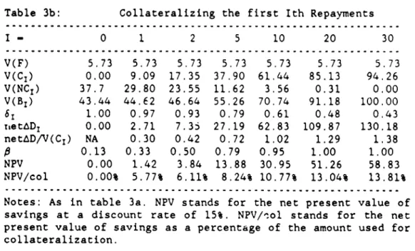
Lamdany and Underwood (1989) use alternative repayment models and show that, even though some differences in the amount of principal and interest reduction exist between buybacks and (different forms of) debt exchange, the present value of debt service savings is largely invariant for a given amount of resources used (and for reasonable discount rates). They also provide cases, where the timing of collateralization becomes important. For example, table 3b present one example where the probability of repayment declines exponentionally over time. As one can observe, the amount of debt reduction per dollar of collateral increases substantially as payments further in the future--those less likely serviced--get collateralized.18
17See Claessens and Diwan (1989) for a discussion.
18To be exact, the marginal debt reduction per added maturity collateralized is equal to the marginal decrease in repayment probability, i.e., d[net,a D/V(C,)]/dI- -dx/dI.
Table 3b: Collateralizing the first Ith Repayments ... ... ... .. .. ... .. I - 0 1 2 5 10 20 30 V(F) 5.73 5.73 5.73 5.73 5.73 5.73 5.73 V(CI) 0.00 9.09 17.35 37.90 61.44 85.13 94.26 V(NC1) 37.7 29.80 23.55 11.62 3.56 0.31 0.00 V(B1) 43.44 44.62 46.64 55.26 70.74 91.18 100.00 61 1.00 0.97 0.93 0.79 0.61 0.48 0.43 TietAD, 0.00 2.71 7.3s 27.19 62.83 109.87 130.18 net&D/V(CI) NA 0.30 0.42 0.72 1.02 1.29 1.38 0 0.13 0.33 0.50 0.79 0.95 1.00 1.00 NPV 0.00 1.42 3.84 13.88 30.95 51.26 58.83 NPV/col 0.00% 5.77% 6.11% 8.24% 10.77% 13.04% 13.81% Notes: As in table 3a. NPV stands for the net present value of savings at a discount rate of 15%. NPV/col stands for the net present value of savings as a percentage of the amount used for
collateralization.
IV Characterizing the Best Debt and Debt Service Reduction Deals
We will consider here the case where the IFIs make available to the country some loans that have to be used for debt and debt service reductions. The country subsequently negotiates with its creditors over different debt and debt and service reduction options and amounts of new money. This section presents a simple methodology to determine the set of new liquidity and debt reduction combinations which leave the creditor banks indifferent to the status quo. These combinations represent the "best" the country can hope to get out of its bargaining with the creditors. We then discuss how the debtor country might be able to determine the combination of new liquidity and debt reduction that maximizes its own welfare.
1. Dilution Mechanisms
When a debtor country uses some cash to buyback its commercial bank debt, and the buyback is publicly announced, the price of debt will rise. All creditors will gain and less debt reduction will occur. More debt reduction would have been possible if some way could be found to buy back debt at prices closer to the pre-deal price.
One way to do this is to ask the remaining creditors to give some concessions to offset the.r gains from the increase in the price of debt. Necessary to make this feasible--without using coercion--is that free-riding is precluded: either a bank participates in debt reduction (buyback) or it provides a "concession". We will define providing extra-new money as a concession.
22
NOTATION
D - total debt
C - extra cash from official lenders to be used for
buybacks
L - liquidity used for domestic purposes
N - extra-new money
C+N-L - amount used for buybacks or collateralization of
exit bonds
a - share of total debt D that will be choose between the
elements of the menu (aD is the base)
R - share of value of the exit bond that is
collateralized ((1-R) is thus the share of the exit bond which is exempt from new money calls)
6 - the exchange ratio of old debt to the new bonds
n - new money call as a percent of exiting debt
AD - Debt reduction
ADnet - Net Debt reduction (We use AnetD - (N + C - L)/(l +5*9 - 6/5*6]
- N - C; and the base left over for providing new money - a[D
-(C + N - L)/ 6*9]).
p - ex-post price
q - alternative price or ex-ante price
When remaining banks provide new money (in the amount N), they will not lose compared to the status quo if the immediate capital loss involved with the
extra new money loans they provide, (1 - p)*N, is not larger than the capital
gain, Ap, on their existing exposure. Remaining banks are in effect "taxed" with a new money call in order for the deal to be no-more desirable than the no-deal situation.
Extra new money has two effects: it lowers the buyback price--because indebtedness increases--and it increases the resources available for debt reduction. It will thus lead to an increase in the amount of debt reduction. However, the extra new money can be used not only for debt buybacks, but also
for domestic needs (consumption or investment).19 The more new money is used for
liquidity purposes the less debt reduction will result.
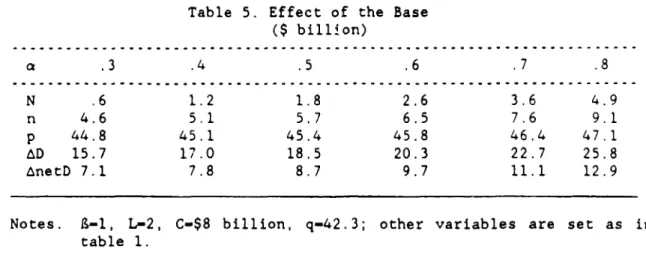
As an illustration, cornsider the situation where D - $100 billion, C - $8
billion (C is the new loan made available by the s for debt reduction) and the
19
When this amount is large, an attempt should be made to integrate in the analysis the effect of the increase in domestic investment on creditworthiness and, thus, on the debt price.
Table 5. Effect of the Base ($ billion) a .3 .4 .5 .6 .7 .8 N .6 1.2 1.8 2.6 3.6 4.9 n 4.6 5.1 5.7 6.5 7.6 9.1 p 44.8 45.1 45.4 45.8 46.4 47.1 AD 15.7 17.0 18.5 20.3 22.7 25.8 AnetD 7.1 7.8 8,7 9.7 11.1 12.9
Notes. B-1, L-2, C-$8 billion, q-42.3; other variables are set as in table 1.
lower exchange ratio 6. When f - 1, the new bond is completely collateralized and the exchange is equivalent to a buyback.
Table 6. The Effect of Leveraging a Debt Exchange ($ billion) 9 .25 .4 .5 .75 1 N .7 1.2 1.4 1.7 1.8 n (percent) 5.7 5.7 5.7 5.7 5.7 p (cents) 45.4 45.4 45.4 45.4 45.4 aD 37.5 28.7 25.5 20.9 18.5 AnetD 8.6 8.6 8.6 8.6 8.6 5 71.6 62.9 58.2 49.0 42.3
Notes: a-.5, L-2, C-$8 billion, q-42.3; other variables as in table 1
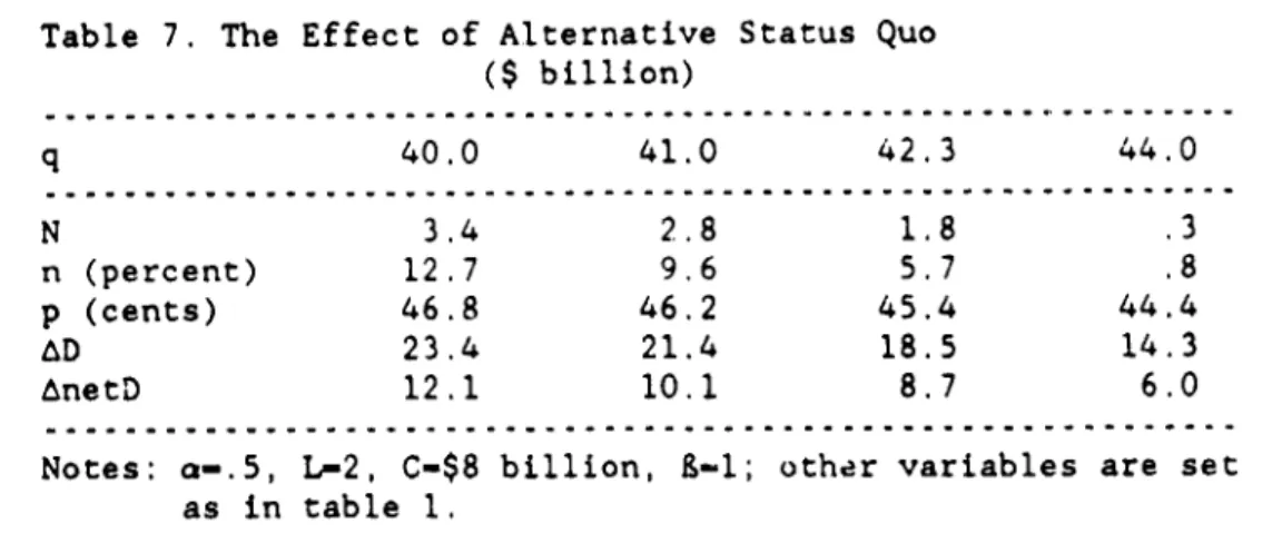
Effect of Alternative Status Quo
The higher the status quo price q (the reservation payoff that the banks must receive), the less net debt reduction a certain amount of resources can accomplish. The lower q, the better the combination of debt reduction-liquidity the country can get. Table 7 shows some sensitivity scenarios with respect to the status quo price q: the amount of new money the banks are willing to provide
28
under the debt deal decreases dramatically with small increases in q.
Table 7. The Effect of Alternative Status Quo ($ billton) q 40.0 41.0 42.3 44.0 N 3.4 2.8 1.8 .3 n (percent) 12.7 9.6 5.7 .8 p (cents) 46.8 46.2 45.4 44.4 AD 23.4 21.4 18.5 14.3 AnetD 12.1 10.1 8.7 6.0
Notes: a-.5, L-2, C-$8 billion, 9-1; other variables are set as in table 1.
5. Applications
5.1 The Recent Mexico Deal
The recent Mexico deal is described in deLail in the box. On 13 September 1989, it was announced that a final agreement was reached. An important part of the agreement was a paragral which stated that the conversion of the base debt
into new instruments throug debt exchanges would explicitly constitute a new contract. The intention of this clause was to imply that the new contracts would no longer be subject to the sharing clauses, could thus receive payments which did not need to be shared with other creditors and would reduce (or even eliminate) the problem of free-riders. This and some pressures of creditor governments appeared in the end to be adequate mechanisms to ensure that (almost) all creditors were coerced into choosing one of the option available.
Mexico Agreement
Mexico and the steering committee of its creditor banks reached an
agreement on July 23 on a debt restructuring package. The package covers about $52.7 billion in medium-term and long-term debt. It offers commercial banks a menu of three options:
(i) a discount bond: a 30 year bond with a discounted principal of 65 percent of the face value of existing debt and an interest rate of LIBOR plus 13/16 percent;
(ii) a par bond: a bond with no discount but a low interest rate of 6.25 percent fixed for the lifetime of the bond; and
(iii) a new money commitment: 7 percent of principal balance at the conclusion of the agreement and 6 percent in 1990, 1991 and 1992, at an interest rate of LIBOR plus 13/16 percent.
The principal of both bonds is guaranteed through the collateralization of a 30-year zero-coupon bond (US-Treasury or its equivalent in case of other currencies). Both bonds are not subject to the sharing clauses which are standard in most syndicated loan agreements.In addition, both bonds include a recapture clause which stipulates that, in case the oil-price
increases by a certain percentage in the years 1997 and. beyond, that the
creditors share in the increased revenue stream. The recapture clause is capped by an amount equal to 3% of the amount of debt exchanged for the two bonds. The agreement also contains a contingent financing facility in case of a decline in oil price. The agreement further specifies a certain number of relending options and a debt-for-equity swap program of at most $1 billion per vear. The agreement was accompanied by the announcement that up to $400 million would potentially be available from the IMF under CCFF arrangen.ents.
Depending on the amounts of debt brought under each option, at least 18 months and at most two years of interest payment is guaranteed on a
rolling basis through an escrow accou1nt. The escrow account is establishied
using the additional firancial support provided by the Bank, the Fund, and Japan and from Mexico's own resources. In total an amount of $7 billion 's used for debt and debt service reduction. Funding comes from the World Bank, IMF, and Japan ($5.3 billion), and from Mexico's own reserves ($1.7 billion).
Banks choose among the options in the fall of 1989 and the final outcome, announced in January 1990, is that out of the $48 billion of bank debt covered by the agreement, 41% will take the principal reduction bonds, 49% the interest reduction bonds, and 10% will provide new money.
30
Evaluation of the deal23
The structure of the deal ensures that banks were coerced to choose one of the options and that non-exiting banks have to contribute with new money, i.e. free-riding has been eliminated. The base debt that had to be divided between the three instruments was relatively large, about half of the total debt was included. One interesting aspect of the deal was that the relative prices of the three options were determined in the steering committee rather than in a
competitive fashion. 24
Using our debt value function, we calculate the status quo debt price at
q - 38.3 (a debt to export ratio of 107/28). The two exit instruments are of
about equal value, slightly above 38.5 cents per dollar of debt. Banks will choose between the two on the basis of their tax, regulatory and accounting regimes. The bonds derive roughly 39 percent of their current value from collateralization.25
Analysis:
We set L - $1.1 billion and, given a, R, q and C - $5.3 billion, find the
amount of new money that leaves the banks indifferent between the discount bond and a one year extra new money call. Our analysis predicts then an extra new
morney amount N of $2.82 billion, an exchange ratio for the discount bond 6 of
62.4 percent and that Mexico uses $1.7 billion of the new money for the purpose of debt reduction, which together with the $5.3 billion from tbe World Bank, the
IMF and Japan, sums up to a total of $7 bi'llion. A total of $34 billion would
theni be exchanged for new bonds, leading to a net debt reduction of $11.7 billion
and a remaining commercial bank debt stock of $18.7 billion. The extra new money
requirement is predicted to be n - 14.4 percent. The total predicted new money
requirement is then 17.5 percent.26 After the deal is completed, the debt price
is expected to rise to p - 41.6.
23
The evaluation of the Mexico was done before the final choices of banks were known (January 1990). The evaluation of this and other deals should largely be viewed as illustrations of .he concepts discussed before. The fact that the results predicted fare well with reality should not be overemphasized as the model itself is onlv rudimentarv.
24A reason that may have plaved a role in this is that US regulators can
oblige banks to reserve against claims according to price bid.
25
The current value of a bond with a face value of $100 consists of three parts: (1) the current value of the two collateralized interest payments ($16.29); (2) the current value of 28 risky interest payments, evaluated at the ex-post price ($35.74); and the current value of the principal collateral
($6.94). The total value of the bond is $58.97 and R, the value of the collateral divided by the value of the bond, is 39 percent.
26This is computed as follows.
A was 0.7 in the last new money agreement,
i.e. banks expected to refinance 30 percent of the interest bill or 3.1 percent of their debt. Adding the extra new monev call (14.4 percent) to this we get a total new money call of 17.5 percent.
The actual distribution over the different options became known in January 1990. The base debt turned out to be $48.4 billion, of which 10% choose the new money opticn, 49% the par bond and 41% the discount bond. Total amount of debt reduction (including the present value of debt service reduction of the par bond) was $15 billion. It looks like the Mexican deal is not far from the debt reduction -liquidity frontier. The analysis revealed that the new money requirement negotiated (25 percent) was too high to be attractive. This may well explain the lack of success of the new money call and why more banks cpted for the debt and debt service reduction instruments. The secondary market price for Mexico was 39.75 in late February, significantly above the levels prevailing before the deal was finalized, in line with our prediction. One important problem with the deal is that it did not specify exactly how to divide the exit instruments if they were over-subscribed, a likely pos3ibility given the slight mispricing that seemed to have occurred.
5.2 The Philippines
Annther country that reached agreement in principle with its commercial banks and that received official support for debt and debt service reduction is the Philippines. The Philippine deal is described in detail in the box. On October 12, the Governor of the Central Bank announced that the Philippines would
Philippine agreement:
The Philippines antiounced on August 15, 1989 that it had reached an agreement in principle with its banks. The agreement stipulated that the Philippines would issue "new money" bonds with the following terms: maturity 15 years, grace 8 vears, spread 13/16 percent over US-dollar 6-months LIBOR. The bonds would not share equally with existing commercial bank debt and the Philippines would covenant not to request restructurings
of the bonds at any time and not to request any new money loans or other financial accommodations from the holders of the bonds. The new money bonds would thus acquire a more senior status.
In addition, the Philippines would be allowed to buyback part of its commercial bank debt in an auction to be held before the issue of the new money bonds.
offer to buy back $1.6 billion of its foreign commercial debt for $800 million, implying a price of 50 cents, and that it planned to borrow about $1 billion through the new money bonds. The announcement also stated that Philippines expected to receive support from the World Bank, the IMF and bilateral donors for about $710 million for the buvback. Banks were given three weeks to respond to the offer. The new-money bond will not be finished after the buyback is completed, which happened in January 1990.
32 Analysis
In terms of our notation, a - 43.9 (bank debt i, $12.5 billion and total
debt is $28.5 billion), q - 50, and I - 1. The status quo price given by our
model (exports of $11 billion) is q - 51.1, implying that a buyback price of
50 cents is about correct (a bit on the low side). Setting C - $710 million and
L - $290 million, the analytical model predicts: N - $309 million, p - 51.8
cents, AD - $1,638 million and netAD - $529 million.
A total of $819 (710-290+399) million will be used for the buyback, reducing debt on net by $529 million. In the past, the Philippines had refinanced
about half its interest payments.2' For $10.9 billion of remaining commercial
debt, this comes to $505 million of expected new money as the alternative
scenario. Adding the extra new money call of $399 million gives a total new money call of $904 million, quite close to what the Philippines are now seeking (given
the reduction in the base--from $12.5 billion to $10.9 billion--this corresponds
to a new money call of 8.3 percent).
5.3 Costa Rica
On October 27 Costa Rica announced that it had reached agreement in principle with its commercial bank creditors on a debt reduction package (see further the box). The pathbreaking agreement was because of its treatment or arrears.
Aralysis
It appears that the Costa Rica agreemeLit handles the free-rider problem
through incentives appropriately. Even though no formal mechanism is put in place to address free-riders, the different treatment of the creditors which will serve as an incentive scheme plus the (explicit) condonment by the IFIs, of arrears to the commercial banks should be sufficient to assure complete
participation.
In terms of our analytical framework we have the following parameters: D
- $4.85 billion (including arrears), commercial bank debt - $1.825 billion,
i.e., a - .38, q - .16 and C - 250 million. The low interest rate on the par
bonds implies approximately 35 cents present value of debt relief per dollar of
face vai.ue. The relative amount of collateral involved in the package of 6.25
27
In our pricing model, a A of 0.5 corresponds to R - 13.7 percent when p
Costa Rica Agreement:
The agreement includes the following elements.
Banks can tender their loans for cash at a price to be announced by Costa Rica. Debt not tendered will be converted into bonds with a 6 1/4 percent annual coupon. On the past due interest (amounting in total to approximately $325 million) not deemed extinguished through the buyback, Coqta Rica will, as the buyback and the exchange take place, make a 20 percent down payment on the (written down) back due interest and pay the rest over 15 years with no grace period and at a spread of 13/16 over money market rates.
Banks tendering 60 percent or more of their exposures are differentiated from the others. Their 6 1/4 percent par bonds will carry a shorter maturity and one year interest guarantee, while their past due interest will carry a three year rolling guarantee. Those banks tendering less than 60 percent will receive no guarantees and their 6 1/4 percent par bonds will carry a longer maturity and grace.
Official support for the program will cover t-he costs of the buyback
and the interest guarantee and is expected to amount to some $250 million. The official support is expected to be provided by the IMF, World Bank, and to come from bilateral sources, including Japan, Taiwan, and the U.S, with possible funds coming from one or two European countries. According to the President of Costa Rica, the agreement will reduce the country's commercial debt by about two-third and its interest bill to the commercial banks by the same proportion, to $50 million.
percent par bonds, X, is approximately 12 percent.28 Setting L - 0, gives the
following results: netAD - $1.35 billion, debt reduction from par bonds - $0.256
billion and the ex-post price is 58.6 cents, significantly above the price for the buyback (16 cents). The results correspond to the expected actual debt reduction which is buybacks of 60 percent leading to $1095 million debt reduction and exit bonds providing $219 million in debt relief, totalling $1314 million.
28Assume that 60 percent of the banks offer 60 percent of their claims for
the buyback and 40 percent for the exit bond (banks A) and that the other 40
percent of the banks choose for 100 percent the exit bond (banks B) . Banks A
receive then on their exit bonds 1 year collateral for the debt part and 20 percent downpavment and 3 years collateral for the past due interest part, implying an average collateralization of about 18 percent. Banks B receive only 20 percent downpayment on their past due interest, implying approximately 4 percent collateralization. The average for banks A and B is then 12 percent,
34
6. Seniority, Prices and Buybacks
The importance of seniority has been pr Lnted out in the discussion on exit
bonds. Changes in the degree of seniority can furthermore have an important impact on the amount of debt reduction that can be achieved in any deal and on the net change in the value of claims of each seniority class. The debt value function that has been used (equation 3) did not account for differences in seniority between commercial bank debt and other debt and was estimated using the secondary market price for commercial bank debt as the average price for all debt. If commercial banks are the most junior creditors, however, the secondary market price would not reflect the average price for all debt, but the price of the debt that is serviced after all other creditors are serviced. The secondary market price would then be below the average price for all debt.
A debt value function which accounts for this seniority structure can be estimated. The procedure used was as follows. Going along the debt value curve, the market value of debt accrues first to the most senior lenders, then to the more junior lenders, and then to the most junior lenders. If we assume that there are only two classes of debt, the market value of the debt of the senior lenders will be the value of debt given by the debt value curve for the face value of their debt only. The market value of the junior creditors will be the market value of total debt minus the market value of the debt of the senior lenders. We can write this as:
V(Dj;a,,6) - V(Di + D,;a,B) - V(D,;a,B) (10)
where DJ is the face value of junior debt, D, is the face value of senior debt,
and where all market values depend on the parameters for the debt value curve
a and B. Since V(D3;a,B) - p(D,;a,6)*D,, where p(D,;Q,O) is the predicted
(secondary market) price for junior debt, this can also be written as:
p(DJ;a,B) - [V(D3 + D,;a,o) - V(Ds:a,3)]/D, (11)
A debt-value which allows for seniority can now be estimated by minimizing the sum of squared errors between predicted and observed secondary market prices,
[p(DJ;a,O) - p]2, over the parameters a and B. The result is as follows:
ln[p/(l-p)] - 7.438 - 1.2134*ln(D/X) (12)
The estimated coefficient for the slope is lower than with the no-seniority curve (1.234 compar-d to 1.44), a reflection of the fact that the debt value curve flattens out less rapidly when the debt-to-export ratio increases. Using our previous example (total debt $100 billion and exports $30 billion) and assuming that debt senior to commercial bank claims is $50 billion, we calculate the average price of all debt, call it t, as 59.6 cents, the price of senior debt, call it s, as 77.4 cents and the price of commercial bank debt p as 41.8 cents. Table 8 provides prices for alternative combinations of total and senior debt.
Prices for total debt are consistently above the prices predicted on the basis of the no-seniority curve (see table 1). The elasticity of the price for bank debt with respect to the total amount of debt is similar to before. The
Table 8. Prices for Alternative Levels 'f Total and Senior Debt (cents) D 80 90 100 110 120 0 50 50 50 50 50 p (banks) 46.8 44.3 41.8 39.6 37.6 t (total) 65.9 62.7 59.6 56.8 54.2 s (senior) 77.4 77.4 77.4 77.4 77.4 D 100 100 100 100 100 0 20 30 40 60 70 t (total) 59.6 59.6 59.6 59.6 59.6 p (banks) 51.7 48.1 44.8 39.1 36.6 s (senior) 91.2 86.4 81.8 73.3 65.9
bottom panel can be used if there exist multiple seniority classes to evaluate the value of debt in each class. For instance, the price of the $20 billion of most senior claims is close to par: 91.2 cents. The price of the next most senior
$10 billion of claims is 76.8 cents. 29 Keeping total debt fixed, the larger the
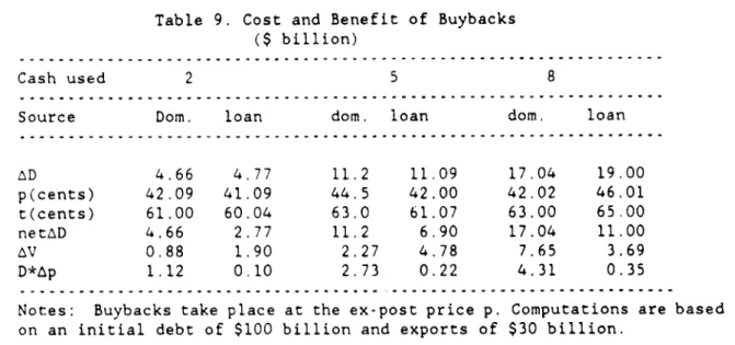
share of senior debt, the lower the price for the commercial bank claims. Thble 9 provides information on the costs and benefits of buybacks done at the ex-post price for commercial bank debt and accounting for the seniority structure. The main difference compared to the no-seniority case is that the ex-post price does not increase as much when a senior loan is used to buy back debt. It is even possible that the price for commercial bank claims will fall as a result of more senior debt, even if total debt is reduced. The net debt reduction when domestic resources are used is larger than before as the price of commercial bank debt rises less.
VI. Conclusions
This paper has presented a simple methodology for identifying the set of best debt deals a country can bargain for with its creditors when debt reduction is included in the set of options. The challenge will now be to identify the deal which is best for the country given its liquidity versus debt reduction preferences while at the same time being acceptable to its creditors. This will
29
This is derived as the total value of the $30 billion in claims ($30
billion * 86.4 cents) minus the value of the $20 billion in claims ($20 billion
36
Table 9. Cost and Benefit of Buybacks
($ billion)
- - - -- - - -.. ..- . ... - . . . .. - - - . . . . ...- - - - -.
Cash used 2 5 8
Source Dom. loan dom. loan dom, loan
AD 4.66 4.77 11.2 11.09 17.04 19.00 p(cents) 42.09 41.09 44.5 42.00 42.02 46.01 t(cents) 61.00 60.04 63.0 61.07 63.00 65.00 netAD 4.66 2.77 11.2 6.90 17.04 11.00 AV 0.88 1.90 2.27 4.78 7.65 3.69 D*Ap 1.12 0.10 2.73 0.22 4.31 0.35
Notes: Buybacks take place at the ex-post price p. Computations are based on an initial debt of $100 billion and exports of $30 billion.
require a general equilibrium macroeconomic model which might provide the necessary framework for analyzing a country's investment, growth and repayments behavior in a situation of a foreign credit constraint and a debt overhang.