04 August 2020
POLITECNICO DI TORINO
Repository ISTITUZIONALE
Training pairwise Support Vector Machines with large scale datasets / Cumani S.; Laface P.. - STAMPA. - 1(2014), pp.
1664-1668. ((Intervento presentato al convegno 2014 IEEE International Conference on Acoustics, Speech, and Signal
Processing ICASSP 2014 tenutosi a Florence (Italy) nel May 4-9, 2014.
Original
Training pairwise Support Vector Machines with large scale datasets
Publisher:
Published
DOI:
Terms of use:
openAccess
Publisher copyright
(Article begins on next page)
This article is made available under terms and conditions as specified in the corresponding bibliographic description in
the repository
Availability:
This version is available at: 11583/2551353 since:
TRAINING PAIRWISE SUPPORT VECTOR MACHINES WITH LARGE SCALE DATASETS
Sandro Cumani and Pietro Laface
sandro.cumani, [email protected]
- Politecnico di Torino, Italy
ABSTRACT
We recently presented an efficient approach for training a Pairwise Support Vector Machine (PSVM) with a suitable kernel for a quite large speaker recognition task. The PSVM approach, rather than es-timating an SVM model per class according to the “one versus all” discriminative paradigm, classifies pairs of examples as belonging or not to the same class. Training a PSVM with large amount of data, however, is a memory and computational expensive task, because the number of training pairs grows quadratically with the number of training patterns. This paper proposes an approach that allows discarding the training pairs that do not essentially contribute to the set of Support Vectors (SVs) of the training set. This selection of training pairs is feasible because we show that the number of SVs does not grow quadratically, with the number of pairs, but only lin-early with the number of speakers in the training set. Our approach dramatically reduces the memory and computational complexity of PSVM training, making possible the use of large datasets, including many speakers. It has been assessed on the extended core conditions of the 2012 Speaker Recognition Evaluation. The results show that the accuracy of the trained PSVMs increases with the training set size, and that the Cprimaryof a PSVM trained with a small subset of
the i–vectors pairs is10−30% better than the one obtained by a generative model trained on the complete set of i–vectors.
Index Terms— Speaker recognition, i–vector, PLDA, Support Vectors, Pairwise Support Vector Machines
1. INTRODUCTION
I–vectors [1], a compact representation of a Gaussian Mixture Model (GMM) supervector [2], in combination with Probabilistic Linear Discriminant Analysis (PLDA) [3, 4], allow speaker recognition sys-tems to reach state–of–the–art performance. A successful alternative to the probabilistic generative PLDA model has been recently pre-sented: a discriminative SVM model trained to decide whether a pair of utterances belongs or not to the same speaker [5, 6]. This is in contrast with the usual “one-versus-all” framework, where an SVM model is created for each enrolled speaker, using as samples of the impostor class the utterances of a background cohort of speak-ers. This approach avoids the major weakness of “one-versus-all” SVM training, namely the scarcity of available samples for the tar-get speakers. Although our pairwise SVM training approach is ex-tremely efficient, it is nevertheless expensive in terms of memory and computational resources, which grow quadratically with the number of the training i–vectors. It is also more challenging than the one– versus–all SVM training, due to the size of the matrix of the scores that must be stored during the training iterations: a set of 256K i– vectors would need approximately 128GB of memory just for the Computational resources for this work were provided by HPC@POLITO (http://www.hpc.polito.it)
lower triangular score matrix. To solve this problem, it is worth re-calling that the solution of the SVM optimization problem, in its dual formulation [7, 8], shows that the separation hyperplane is a function of a subset of training patterns, the so-called Support Vectors (SVs). Since it is known that the number of SVs increases linearly with the number of training patterns [9], several solutions have been pro-posed in the past to reduce their number, aiming at eliminating the SVs that are not essential [10] or the SVs recognized as unnecessary, being linearly dependent in feature space [11]. These approaches try to reduce the number of SVs for a generic SVM binary problem. The problem that we address, instead, is characterized by a small number of utterances, pronounced by a large number of speakers, and by two highly unbalanced classes: the “same speaker” pairs, which grows linearly with the number of speakers, and the “differ-ent speaker” pairs, which grows quadratically with the number of i–vectors. For this specific task, we propose a simple solution that allows discarding the training i–vector pairs that do not essentially contribute to the set of SVs. In particular, since the amount of mem-ory required for training a generative PLDA model is not affected by the size of the training set, we first train a PLDA model with the complete set of training i–vectors. Then, the scores of the training pairs are computed using this PLDA model, and all pairs with a score less than a threshold are removed from the training list of the PSVM. The rationale for this approach is that there is good correlation be-tween the PLDA and the PSVM scores. Thus, “different speaker” i–vector pairs with large negative PLDA scores, and “same speaker” i–vector pairs with large positive PLDA scores, do not contribute to the set of SVs.
Please notice that this selection strategy is feasible only because we show that the number of SVs does not increases quadratically, with the number of the i–vector pairs, but only linearly with the num-ber of training speakers. This makes our approach not only feasi-ble, but also extremely efficient: by keeping a very small fraction of the training pairs, a dramatic reduction of the memory and com-putational complexity of PSVM training is obtained without losing accuracy. The experimental results confirm that the accuracy of the trained PSVMs increases using more speakers in the training set, making the proposed approach effective both for its reduced com-plexity and for its obtained performance.
The outline of the paper is as follows: Sections 2 formulates the i–vector pair score as a second order Taylor approximation of a symmetric score function. Section 3 describes the pairwise SVM classifier, and its efficient implementation. In Section 4 we detail our selection strategy. Section 5 presents the experimental results, comparing the performance of the PLDA models and of the PSVM models trained with a selected subset of pairs. Our conclusions are drawn in Section 6.
2. I–VECTOR PAIR SCORE APPROXIMATION
It has been shown in [6] that the score of the i–vector pairΦ = (φ1,φ2)can be formulated as a functions(Φ), invariant to i–vector
swapping. This formulation is here recalled for introducing the hyper–parameters that a SVM must estimate, and for illustrating the changes necessary for training a PSVM with a reduced dataset. The second order Taylor expansion fors(Φ)around pointΦˆ =0 is:
s(Φ) =s( ˆΦ) + (Φ·∇s|Φˆ) +Φ
T
(H(s)|Φˆ)Φ, (1)
where∇is the vector of differential operators∇=∂∂Φ
1, . . . ,
∂ ∂Φd
,
dis the dimension of the i–vector pair, andH(s)is the Hessian of functions(Φ). Defining: s( ˆΦ) =k , ∇s|Φˆ = [c c], H(s)|Φˆ = Γ Λ Λ Γ , (2)
with a symmetricΛ, we obtain the quadratic function of the i–vector pair: s(φ1,φ2) = φ T 1Λφ2+φ T 2Λφ1+φ T 1Γφ1+φ T 2Γφ2 +(φ1+φ2) T c+k , (3)
which can be also interpreted as a linear function of the hyper– parameter setΘ ={Λ,Γ,c, k}, in an expanded space of i–vector pairs. In particular,s(φ1,φ2)can be written as the dot–product of a
vector of weightsw(the model hyper–parameters) and an expanded vectorϕ(φ1,φ2)representing an i–vector pair:
s(φ1,φ2) =wTϕ(φ1,φ2). (4)
where the parameters and the expanded i–vector pair are represented using thevec(·)operator, which stacks the columns of a matrix into a vector, as: w= vec(Λ) vec(Γ) c k , ϕ(φ1,φ2) = vec(φ1φT2 +φ2φT1) vec(φ1φT1 +φ2φT2) φ1+φ2 1 . (5) 3. PAIRWISE SVM TRAINING
A linear SVM can be trained to learn these model hyper–parameters, however, training by means of a dual solver [12, 13] has severe limi-tations for large training sets. Caching the complete kernel matrix is impractical even for relatively small sized datasets because it would requireO(n4)memory, wherenis the number of i–vectors. Also impractical are the alternatives of keeping in memory the complete dataset of mapped features (O(n2d2)), wheredis the i–vector di-mension, or expanding the features on–line, with a computational complexityO(n2d2)for each iteration. Since in NIST SRE 2010, for example, a popular setting for the i–vector dimension isd= 400, and the number of training i–vectorsnis approximately 20000, us-ing a standard SVM dual solver approach would be impractical. It has been shown in [6, 14] that the kernel formulation depends only on i–vector dot–products, so that kernel can be efficiently computed by caching the i–vector Gram–matrix. The memory cost, however, remainsO(n2)
.
We use instead a primal solver because it has been shown in [6] that it is possible to efficiently evaluate the loss function and its gra-dient with respect towover the set of all training pairs, inO(n2d+ nd2)time, without the need of expanding the i–vectors. An analysis of large-scale SVM training algorithms suited to speaker recogni-tion tasks [15] allowed us to select, among the primal solvers, the Optimized Cutting Plane Algorithm (OCAS) approach proposed in [16, 17], which offers a general and easily extensible framework for
solving convex unconstrained regularized risk minimization prob-lems. Although the memory cost remainsO(n2)even for a primal
solver, the i–vector pair selection strategy, illustrated in the next sec-tion, allows memory complexity to be dramatically reduced.
Our formulation is also equivalent to a second degree inhomoge-neous polynomial kernel SVM. Pairwise SVM training using poly-nomial kernel SVMs has been also proposed in [14] for medium sized training sets. As it is shown in Section 4, our selection strategy makes PSVM training much less expensive, and feasible with very large training sets.
SVM optimization can be seen as the solution of the uncon-strained convex regularized risk minimization problem:
E(w) = arg min w 1 2λkwk 2 +1 n n X i=1 `(w,xi, ζi) (6)
with loss function
`L1(i) = max(0,1−ζiwTxi). (7)
Using the OCAS technique, the SVM parametersware optimized by evaluating the loss function and a sub–gradient of its objective function (6). These evaluations require, in principle, a sum over all the expanded i–vector pairs in the training set. Since their number isn2, which can easily reach the order of hundred of millions for typical training sets, these evaluations would be not effective or even feasible because their complexity would beO(n2d2).
However, the objective function and its gradient can be com-puted by means of a much more efficient solution in terms of mem-ory and computation using (3). In particular, letD= [φ1φ2. . .φn]
be a matrix includingnstacked i–vectors, and letSθ i,j =Sθ(φi,φj)
denote the score matrix for all possible pairs related to componentθ
ofw, whereθ ∈ {Λ,Γ,c, k}. From (4) and (3) the score matrices can be evaluated as:
SΛ(φi,φj) =φ T iΛφj+φ T jΛφi⇒SΛ= 2DTΛ D SΓ(φi,φj) =φ T iΓφi+φ T jΓφj⇒SΓ= ˜SΓ+ ˜SΓ T Sc(φi,φj) =c T (φi+φj) ⇒Sc= ˜Sc+ ˜Sc T (8) Sk(φi,φj) =k ⇒Sk=k·1, where ˜ SΓ= [dΓ. . . dΓ | {z } n ] S˜c= [dc. . . dc | {z } n ], (9) and dΓ=diag(DTΓD) dc=DTc. (10)
Thediag(·)operator returns the diagonal of a matrix as a column vector, and1is ann×nmatrix of ones.
No explicit expansion of i-vectors is, thus, necessary for evaluating the scores.
Denoting the sum of the partial score matrices byS = SΛ+
SΓ+Sc+Sk, the SVM loss function can be obtained as:
`L1(D,Z) =
X
i,j
max[0,1−ζi,jwTϕ(φi,φj)]
= h1,max[0,1−(Z◦S)]i, (11) where0is ann×nmatrix of zeros,Zis then×nmatrix of the labelsζi,jfor each i–vector pair(φi,φj), and◦is the element-wise
matrix multiplication operator.
Fig. 1: Percentage of Support Vectors as a function of the percentage of the training i–vectors.
the derivative of the hinge loss function with respect to the score
si,j=wTϕ(φi,φj): gi,j= ( 0 ifζi,jsi,j ≥1 −ζi,j otherwise. (12) LetGbe the matrix of the elementsgi,j. Recalling thatGis
sym-metric, the terms of the sub–gradient of the loss function can be rewritten in terms of dot–products and element–wise matrix prod-ucts as: ∇`w= 2 vec DGDT 2 vec [D◦(1AG)]DT 2 [D◦(1AG)] 1B 1T BG 1B , (13)
where1Ais ad×nmatrix of ones, and1Bis a sizencolumn vector of ones.
Again, no explicit expansion of i-vectors is necessary for this evalu-ation.
Due to the small size of the i–vectors, the dataset of training ut-terances can easily be loaded in main memory. The evaluation of loss functions and gradients in OCAS, thus, requires matrix–by–matrix multiplications of large matrices (n×n), which can also be loaded in main memory ifnis not too large. Although, for a very large training set, these computations can be performed through block decompo-sition of the matrices, this procedure is cumbersome and slow. The selection strategy illustrated in the next section solves these memory problems, and allows training a pairwise SVM even with millions of i–vectors of a very large set of speakers. The terms in (8), and the loss function (11), are computed only for the selected pairs, and the elements ofGcorresponding to discarded pairs are set to0in (13). Since their number is very high, a sparse matrix representation is used.
4. I–VECTOR PAIR SELECTION
Although a dual solver is not used by our approach, we will make use of the definition of Support Vector to devise an effective selec-tion strategy. Our strategy is based on two main observaselec-tions, and a working hypothesis, confirmed by experimental evidence. The first observation is that the PSVM support vectors are a small fraction of the complete training set. The second observation is that the scores of the generative PLDA models are correlated with the scores of a PSVM trained with the same training set. The working hypothesis is that it is possible to a–priori identify and discard most of the i–vector pairs that do not contribute to the set of SVs of the complete training set.
In particular, a proof, omitted here for lack of space, can be given that the number of support vectors in a SVM is upper bounded by a linear function of the number of elements of the less popu-lated class. In speaker recognition, the training set typically includes a quite large number of speakers, each providing a small number of utterances. Thus, the less populated class is the “same speaker”
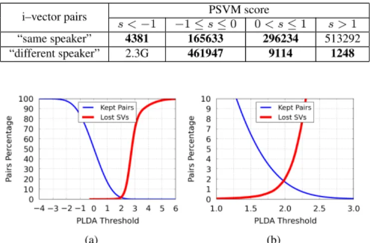
Table 1: Distribution of the number of “same speaker” and “different speaker” i–vector pairs in the regions defined by the margins of a PSVM. The number of SVs is shown in bold.
i–vector pairs PSVM score
s <−1 −1≤s≤0 0< s≤1 s >1
“same speaker” 4381 165633 296234 513292
“different speaker” 2.3G 461947 9114 1248
(a) (b)
Fig. 2: (a) Percentage of i–vector pairs that are included in the PSVM training set, and percentage of lost support vectors, as a func-tion of the PLDA score threshold. (b) Zoom of a region of (a)
class, which grow linearly with the number of speakers, whereas the cardinality of the “different speaker” class is much larger because it grow quadratically with the number of i–vectors. Using the the set of 48568 i–vectors described in Section 5, we have approximately 2.3 billion “different speaker”, and one million “same speaker” pairs. Figure 1 plots (in percentage) the number of SVs obtained by train-ing a PSVM with the i–vectors of an increastrain-ing number of speakers. The figure confirms our theoretical claim that the number of SVs grows linearly with the number of i–vectors (n) rather than with the number of the training set pairs (n2).
Training a PSVM with the complete training set, and computing the PSVM scoresof each i–vector pair of the same set, we obtained the distribution of the number of i–vectors in the regions defined by the PSVM margins. The distribution is reported in Table 1, where the number of SVs for each class is shown in bold. It is worth noting that although the number of “different speaker” pairs is much greater than the number of “same speaker” pairs, this is not the case for the number of the corresponding SVs, which is similar.
The correlation coefficient between the scores of the PSVM and of a PLDA trained on the same set of pairs are0.83and0.69, for the “same speaker” and “different speaker” classes, respectively. Figure 2 shows the percentage of i–vector pairs that would remain on the training set, and the percentage of SVs that would be discarded, as a function of a threshold on the PLDA scores. It is worth noting that it is sufficient to keep a small fraction of the complete training set to include almost all the SVs of the complete training set in the filtered training set. This implies that the PSVM solution obtained with the small subset of selected training pairs will need much less memory and processing time, but will be nevertheless near optimal.
These considerations allow us to devise a simple strategy for detecting and discarding the subset of i–vectors which have few chances to be SVs for the PSVM. It is based on the evidence that the number of support vectors grows linearly with the number of “same speaker” pairs. In particular, the complete set of training pairs is classified using a PLDA model trained on the same data, and only theK–best scoring pairs are kept as training set for the
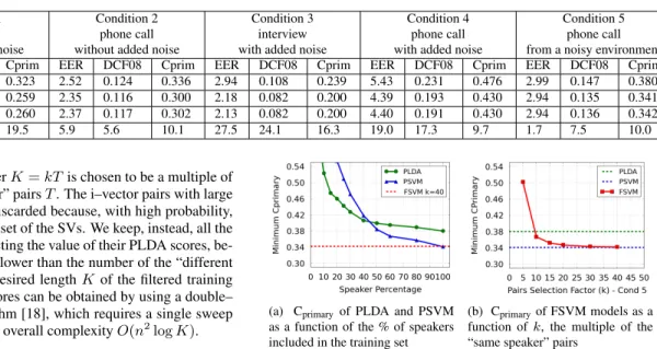
Table 2: Performance of gender independent PLDA and PSVM models, trained with full, and filtered training sets, on NIST 2012 extended core evaluation. Last row gives the % performance improvement of the FSVM models with respect to the PLDA.
Model
Condition 1 Condition 2 Condition 3 Condition 4 Condition 5
interview phone call interview phone call phone call
without added noise without added noise with added noise with added noise from a noisy environment
EER DCF08 Cprim EER DCF08 Cprim EER DCF08 Cprim EER DCF08 Cprim EER DCF08 Cprim
PLDA 3.76 0.160 0.323 2.52 0.124 0.336 2.94 0.108 0.239 5.43 0.231 0.476 2.99 0.147 0.380
PSVM 2.71 0.108 0.259 2.35 0.116 0.300 2.18 0.082 0.200 4.39 0.193 0.430 2.94 0.135 0.341
FSVM 2.66 0.108 0.260 2.37 0.117 0.302 2.13 0.082 0.200 4.40 0.191 0.430 2.94 0.136 0.342
% impr. 29.3 32.5 19.5 5.9 5.6 10.1 27.5 24.1 16.3 19.0 17.3 9.7 1.7 7.5 10.0
PSVM model. The parameterK=kTis chosen to be a multiple of the number of “same speaker” pairsT. The i–vector pairs with large negative PLDA scores are discarded because, with high probability, they do not contribute to the set of the SVs. We keep, instead, all the “same speaker” pairs, neglecting the value of their PLDA scores, be-cause their number is much lower than the number of the “different speaker” pairs. Given the desired lengthKof the filtered training set list, the top-KPLDA scores can be obtained by using a double– ended priority queue algorithm [18], which requires a single sweep of the PLDA scores, with an overall complexityO(n2logK).
5. EXPERIMENTAL RESULTS
Since our experiments were focused on memory and computational cost of PSVM training, we did not devote particular care to select the best combination of features, techniques, and training data that al-low obtaining optimal performance. Every utterance was processed after Voice Activity Detection, extracting every 10 ms, 19 Mel fre-quency cepstral coefficients, and the frame log-energy on a 25 ms sliding Hamming window. This 20–dimensional feature vector was subjected to short time mean and variance normalization using a 3 s sliding window, and a 45-dimensional feature vector was obtained by stacking 18 cepstral (c1-c18), 19 delta (∆c0-∆c18) and 8 double–
delta (∆∆c0-∆∆c7) parameters. We trained a gender–independent
i–vector extractor, based on a 1024–component diagonal covariance gender–independent UBM, and on a gender-independentTmatrix, estimates with data from NIST SRE 2004–2010, and additionally with the Switchboard II, Phases 2 and 3, and Switchboard Cellular, Parts 1 and 2 datasets, for a total of 66140 utterances. The i-vector dimension was fixed tod= 400. The PLDA and SVM models were trained using the NIST SRE 2004–2010 datasets, for a total of 48568 utterances of 3271 speakers. The enrollment part of the NIST 2102 dataset was not used because the complete set would become too large for training the PSVM reference system.
We trained PLDA models with full–rank channel factors, using 200 dimensions for the speaker factors. The i–vectors of the PLDA models were whitened andL2 normalized. Within Class Covari-ance Normalization (WCCN) [19] was applied to the i–vectors for the PSVM. The WCCN transformations and the PLDA models have been trained using the previously mentioned NIST datasets. These systems were tested on the extended core NIST 2012 evaluation tri-als [20]. The scores were not normalized.
Table 2 summarizes the performance of three models, in terms of % Equal Error Rate, minimum Decision Cost Function, and minimum Cprimary, defined for the NIST 2008 and 2012 evaluations
[20]. The result are shown for the reference PLDA model, for the PSVM model trained with the complete set, and for a pairwise SVM (FSVM) trained with a filtered set of sizeK = 40T, where
T = 979540is the number of “same speaker” pairs. The FSVM model performs similarly to the PSVM, and better than PLDA mod-els, in all conditions. Figure 3a plots the minimum Cprimaryof PLDA
(a) Cprimary of PLDA and PSVM
as a function of the % of speakers included in the training set
(b) Cprimaryof FSVM models as a
function ofk, the multiple of the “same speaker” pairs
Fig. 3: Performance comparison of PLDA and of pairwise SVM models on Condition 5 of NIST 2012 evaluation.
and PSVM models trained with utterances provided by an increas-ing number of speakers, for Condition 5. The generative models of PLDA are better than PSVM models if trained with small subsets of the speakers, whereas the PSVM models prevail when the training set includes enough speakers (50% in our experiments). The results of these PSVM models, trained with a reduced set of speakers, con-firm that discriminative training needs a sufficient variety of speakers to avoid overfitting, but is able to outperform PLDA models. The horizontal dashed line shows that a FSVM trained with the PLDA
40T–best scoring pairs, is able to reach the performance of a PSVM trained with the complete training set, but with a 60 times reduction of the memory costs. Figure 3b shows the behavior of minimum Cprimary of a FSVM trained with different filtered set of i–vectors,
each obtained according to our proposed approach. The number of the selected i–vectors in the set is a multiple of the number of “same speaker” pairsT. Usingk = 10, i.e., just10times the number of “same speaker” pairs, our FSVM model outperforms PLDA, and increasing the factork, it rapidly reaches the PSVM accuracy.
6. CONCLUSIONS
A simple and effective approach for the elimination of the i–vector pairs that are not essential in training a pairwise SVM has been pre-sented. We addressed the computational and memory issues raised by the quadratic increase of the i–vector pairs, showing that the num-ber of support vectors is bounded by a linear function of the numnum-ber of “same speaker” pairs, thus it does not increase quadratically with the number of i–vectors, but linearly with the number of speakers. Using this i–vector pairs selection approach, PSVM training with the utterances of a very large set of speakers becomes feasible. This is important because we have shown that FSVM benefits from the use of additional data of different speakers, and that the FSVM mod-els trained with a large enough training set can perform better than PLDA models.
7. REFERENCES
[1] N. Dehak, P. Kenny, R. Dehak, P. Dumouchel, and P. Ouel-let, “Front–end factor analysis for speaker verification,”IEEE Transactions on Audio, Speech, and Language Processing, vol. 19, no. 4, pp. 788–798, 2011.
[2] D. A. Reynolds, T. F. Quatieri, and R. B. Dunn, “Speaker veri-fication using adapted Gaussian Mixture Models,”Digital Sig-nal Processing, vol. 10, no. 1-3, pp. 31–44, 2000.
[3] S. J. D. Prince and J. H. Elder, “Probabilistic Linear Discrimi-nant Analysis for inferences about identity,” inProceedings of 11th International Conference on Computer Vision, 2007, pp. 1–8.
[4] P. Kenny, “Bayesian speaker verification with Heavy– Tailed Priors,” in Keynote presentation, Odyssey 2010, The Speaker and Language Recognition Workshop, 2010, Available athttp://www.crim.ca/perso/patrick. kenny/kenny_Odyssey2010.pdf.
[5] S. Cumani, N. Br¨ummer, L. Burget, and P. Laface, “Fast Dis-criminative Speaker Verification in the i–vector Space,” in Pro-ceedings of ICASSP 2011, 2011, pp. 4852–4855.
[6] S. Cumani, N. Br¨ummer, L. Burget, P. Laface, O. Plchot, and V. Vasilakakis, “Pairwise Discriminative Speaker Verification in the I-Vector Space,” IEEE Transactions on Audio, Speech, and Language Processing, vol. 21, no. 6, pp. 1217–1227, 2013. [7] Vladimir N. Vapnik, The nature of statistical learning theory, Springer-Verlag New York, Inc., New York, NY, USA, 1995. [8] Corinna Cortes and Vladimir Vapnik, “Support-Vector
Net-works,”Machine Learning, vol. 20, no. 3, pp. 273–297, 1995. [9] I. Steinwart, “Sparseness of Support Vector Machines,” JOUR-NAL OF MACHINE LEARNING RESEARCH, vol. 4, pp. 1071–1105, 2003.
[10] G.H. Bakr, L. Bottou, and J. Weston, “Breaking SVM com-plexity with cross training,” inProc. of NIPS 2005, 2005. [11] T. Downs, K.E. Gates, and A. Masters, “Exact simplification
of support vector solutions,”Journal of Machine Learning Re-search, vol. 2, pp. 293–297, 2001.
[12] T. Joachims, “Making large–scale Support Vector Machine learning practical,” inAdvances in Kernel Methods – Support Vector Learning. 1999, pp. 169–184, MIT–Press.
[13] C. Chang and C. Lin, “LIBSVM: a Library for Support Vec-tor Machines,” ACM Transactions on Intelligent Systems and Technology 2 (3), vol. 2, no. 3, 2001.
[14] S. Yaman and J. Pelecanos, “Using Polynomial Kernel Sup-port Vector Machines for Speaker Verification,” IEEE Signal Processing Letters, vol. 20, no. 9, pp. 901–904, 2013. [15] S. Cumani and P. Laface, “Analysis of Large–Scale SVM
Training Algorithms for Language and Speaker Recognition,” IEEE Transactions on Audio, Speech, and Language Process-ing, vol. 20, no. 5, pp. 1585–1596, 2012.
[16] V. Franc and S. Sonnenburg, “Optimized cutting plane algo-rithm for Support Vector Machines,” inProceedings of ICML 2008, 2008, pp. 320–327.
[17] C. H. Teo, A. Smola, S. V. Vishwanathan, and Q. V. Le, “Bun-dle Methods for Regularized Risk Minimization,” J. Mach. Learn. Res., vol. 11, pp. 311–365, March 2010.
[18] S. Sahni, Data Structures, Algorithms and Applications in Java, McGraw-Hill, Inc., 1999.
[19] A. Hatch, S. Kajarekar, and A. Stolcke, “Within-Class Covari-ance Normalization for SVM-Based Speaker Recognition,” in Proceedings of ICSLP 2006, 2006, pp. 1471–1474.
[20] “The NIST Year 2012 Speaker Recognition Evaluation Plan,” Available at"http://www.nist.gov/itl/iad/mig/ upload/NIST_SRE12_evalplan-v17-r1.pdf.