warwick.ac.uk/lib-publications
Manuscript version: Author’s Accepted Manuscript
The version presented in WRAP is the author’s accepted manuscript and may differ from the
published version or Version of Record.
Persistent WRAP URL:
http://wrap.warwick.ac.uk/140441
How to cite:
Please refer to published version for the most recent bibliographic citation information.
If a published version is known of, the repository item page linked to above, will contain
details on accessing it.
Copyright and reuse:
The Warwick Research Archive Portal (WRAP) makes this work by researchers of the
University of Warwick available open access under the following conditions.
Copyright © and all moral rights to the version of the paper presented here belong to the
individual author(s) and/or other copyright owners. To the extent reasonable and
practicable the material made available in WRAP has been checked for eligibility before
being made available.
Copies of full items can be used for personal research or study, educational, or not-for-profit
purposes without prior permission or charge. Provided that the authors, title and full
bibliographic details are credited, a hyperlink and/or URL is given for the original metadata
page and the content is not changed in any way.
Publisher’s statement:
Please refer to the repository item page, publisher’s statement section, for further
information.
Exoplanet Validation with Machine Learning: 50 new
validated Kepler planets
David J. Armstrong,
1,2?Jevgenij Gamper,
3,4Theodoros Damoulas
4,5,61Department of Physics, University of Warwick, Gibbet Hill Road, Coventry, CV4 7AL, UK
2Centre for Exoplanets and Habitability, University of Warwick, Gibbet Hill Road, Coventry CV4 7AL, UK
3Mathematics of Systems CDT, University of Warwick, Gibbet Hill Road, Coventry CV4 7AL, UK
4Department of Computer Science, University of Warwick, Gibbet Hill Road, Coventry CV4 7AL, UK
5Department of Statistics, University of Warwick, Gibbet Hill Road, Coventry CV4 7AL, UK
6The Alan Turing Institute, London, UK
Accepted . Received
ABSTRACT
Over 30% of the∼4000 known exoplanets to date have been discovered using
‘valida-tion’, where the statistical likelihood of a transit arising from a false positive (FP), non-planetary scenario is calculated. For the large majority of these validated planets
calculations were performed using thevespaalgorithm (Morton et al. 2016).
Regard-less of the strengths and weaknesses of vespa, it is highly desirable for the catalogue
of known planets not to be dependent on a single method. We demonstrate the use of machine learning algorithms, specifically a gaussian process classifier (GPC) rein-forced by other models, to perform probabilistic planet validation incorporating prior probabilities for possible FP scenarios. The GPC can attain a mean log-loss per sample
of 0.54 when separating confirmed planets from FPs in the Kepler threshold crossing
event (TCE) catalogue. Our models can validate thousands of unseen candidates in seconds once applicable vetting metrics are calculated, and can be adapted to work
with the active TESS mission, where the large number of observed targets
necessi-tates the use of automated algorithms. We discuss the limitations and caveats of this
methodology, and after accounting for possible failure modes newly validate 50Kepler
candidates as planets, sanity checking the validations by confirming them withvespa
using up to date stellar information. Concerning discrepancies with vespa arise for
many other candidates, which typically resolve in favour of our models. Given such issues, we caution against using single-method planet validation with either method until the discrepancies are fully understood.
Key words: methods: data analysis, methods: statistical, planets and satel-lites:detection, planets and satellites:general
1 INTRODUCTION
Our understanding of exoplanets, their diversity and pop-ulation has been in large part driven by transiting planet surveys. Ground based surveys (e.g. Bakos et al. 2002; Pol-lacco et al. 2006; Pepper et al. 2007; Wheatley et al. 2017) set the scene and discovered many of the first exoplanets. Planet populations, architecture and occurrence rates were exposed by the groundbreaking Kepler mission (Borucki 2016), which to date has discovered over 2300 confirmed or validated planets, and was succeeded by its follow-on K2 (Howell et al. 2014). Now the TESS mission (Ricker et al.
2015) is surveying most of the sky, and is expected to at least double the number of known exoplanets.
The planet discovery process has a number of distinct steps, which have evolved with the available data. Surveys typically produce more candidates than true planets, in some cases by a large factor. FP scenarios produce signals that can mimic that of a true transiting planet (Santerne et al. 2013; Cabrera et al. 2017). Key FP scenarios include various configurations of eclipsing binaries, both on the tar-get star and on unresolved background stars, which when blended with light from other stars can produce eclipses very similar to a planet transit. Systematic variations from the instrument, cosmic rays or temperature fluctuations can produce apparently significant periodicities which are
poten-tially mistaken for small planets, especially at longer orbital periods (Burke et al. 2019; Thompson et al. 2018; Burke et al. 2015).
Given the problem of separating true planetary signals from FPs, vetting methods have been developed to select the best candidates to target with often limited follow-up re-sources (Kostov et al. 2019) . Such vetting methods look for common signs of FPs, including secondary eclipses, centroid offsets indicating background contamination, differences be-tween odd and even transits and diagnostic information re-lating to the instrument (Twicken et al. 2018). Ideally, vet-ted planetary candidates are observed with other methods to confirm an exoplanet, often detecting radial velocity varia-tions at the same orbital period as the candidate transit (e.g. Cloutier et al. 2019).
With the advent of the Kepler data, a large number of generally high quality candidates became available, but in the main orbiting faint host stars, with V magnitude
> 14. Such faint stars preclude the use of radial veloci-ties to follow-up most candidates, especially for long period low signal-to-noise cases. At this time vetting methodologies were expanded to attempt planet ‘validation’, the statistical confirmation of a planet without necessarily obtaining extra data (e.g. Morton & Johnson 2011). Statistical confirma-tion is not ideal compared to using independent discovery techniques, but allowed the ‘validation’ of over 1200 planets, over half of theKepler discoveries, either through consider-ation of the ‘multiplicity boost’ or explicit considerconsider-ation of the probability for each FP scenario. Once developed, such methods proved useful both for validating planets and for prioritising follow-up resources, and are still in use even for bright stars where follow-up is possible (Quinn et al. 2019; Vanderburg et al. 2019).
There are several planet validation techniques in the literature: PASTIS (Santerne et al. 2015; D´ıaz et al. 2014),
BLENDER (Torres et al. 2015), vespa (Morton & Johnson 2011; Morton 2012; Morton et al. 2016), the newly released TRICERATOPS (Giacalone & Dressing 2020) and a spe-cific consideration of Kepler ’s multiple planetary systems (Lissauer et al. 2014; Rowe et al. 2014). Each has strengths and weaknesses, but onlyvespahas been applied to a large number of candidates. This dependence on one method for
∼30% of the known exoplanets to date introduces risks for all dependent exoplanet research fields, including in planet formation, evolution, population synthesis and occurrence rates. In this work we aim to introduce an independent val-idation method using machine learning techniques, particu-larly a gaussian process classifier (GPC).
Our motivation for creating another validation tech-nique is threefold. First, given the importance of designat-ing a candidate planet as ’true’ or ’validated’, independent methods are desirable to reduce the risk of algorithm depen-dent flaws having an unexpected impact. Second, we develop a machine learning methodology which allows near instant probabilistic validation of new candidates, once lightcurves and applicable metadata are available. As such our method could be used for closer to real time target selection and pri-oritisation. Lastly, much work has been performed recently giving an improved view of theKepler satellite target stars through GAIA, and in developing an improved understand-ing of the statistical performance and issues relatunderstand-ing to Ke-pler discoveries (e.g. Bryson & Morton 2017; Burke et al.
2019; Mathur et al. 2017; Berger et al. 2018). We aim to incorporate this new knowledge into our algorithm and so potentially improve the reliability of our results over previ-ous work, in particular in the incorporation of systematic non-astrophysical FPs.
We initially focus on theKepler dataset with the goal of expanding to create a general code applicable to TESS
data in future work. Due to the speed of our method we are able to take the entire threshold crossing event (TCE) catalogue of Kepler candidates (Twicken et al. 2016) as our input, as opposed to the typically studiedKeplerobjects of interest (KOIs) (Thompson et al. 2018), in essence poten-tially replacing a large part of the planet detection process from candidate detection to planet validation.
Past efforts to classify candidates in transit surveys with machine learning have been made, using primarily ran-dom forests (McCauliff et al. 2015; Armstrong et al. 2018; Schanche et al. 2018; Caceres et al. 2019) and convolutional neural nets (Shallue & Vanderburg 2018; Ansdell et al. 2018; Dattilo et al. 2019; Chaushev et al. 2019; Yu et al. 2019; Osborn et al. 2019). To date these have all focused on iden-tifying FPs or ranking candidates within a survey. We build on past work by focusing on separating true planets from FPs, rather than just planetary candidates, and in doing so probabilistically to allow planet validation.
Section 2 describes the mathematical framework we em-ploy for planet validation, and the specific machine learning models used. Section 3 defines the input data we use, how it is represented, and how we define the training set of data used to train our models. Section 4 describes our model se-lection and optimisation process. Section 5 describes how the outputs of those models are converted into posterior probabilities, and combined with a priori probabilities for each FP scenario to produce a robust determination of the probability that a given candidate is a real planet. Section 6 shows the results of applying our methodology to the Ke-pler dataset, and Section 7 discusses the applicability and limitations of our method, as well as its potential for other datasets.
2 FRAMEWORK
2.1 Overview
Consider training dataset D = {xn, sn}Nn=1 containing N
TCEs andxn∈Rdthe feature vector of vetting metrics and
parameters derived from theKeplerpipeline. Letp(X,s) be the joint density, of the feature array X, and the genera-tive hypothesis labels s where s is the array of labels (i.e. planet, or FPs such as an eclipsing binary or hierarchical eclipsing binary). Generative modelling of the joint density has been the approach taken in the previous literature for exoplanet validation, see for example PASTIS (D´ıaz et al. 2014; Santerne et al. 2015) where the generative probability for hypothesis labels has been explicitly calculated using Bayes formula.
The scenarios in question represent the full set of po-tential astrophysical and non-astrophysical causes of the ob-served candidate signal. Let P(s|I) represent the empiri-cal prior probability that a given scenarios has to occur, wheres= 1 represents a confirmed planet ands= 0 refers
to the FP hypothesis, including all astrophysical and non-astrophysical FP situations which could generate the ob-served signal. I refers toa priori available information on the various scenarios.
We implement several machine learning classification modelsMdiscussed in Section 4, with their respective pa-rameters wM. The approaches we take typically estimate
the posterior predictive probability p(s = 1|x∗,D,M) for an unseen feature vector x∗ directly as the result of the classification algorithm. We then obtain the scenario pos-terior probability p(s = 1|x∗,I) by re-weighting using the estimated empirical priors:
p(s= 1|x∗,I) =p(s= 1|x ∗ ,D,M)P(s= 1|I) P sp(s|x ∗,D,M)P(s|I) (1)
where the posterior predictive probability of interest
p(s= 1|x∗,D,M) is given by:
Z
p(s= 1|x∗,wM,M)p(wM|D,M)dwM (2)
and p(wM|D,M) is the parameter posterior for
para-metric models that is typically approximated in Bayesian classification models with an approximating family. Going forwardsD,Mwill be dropped from our notation for clar-ity.
For non-Bayesian parametric methods the marginal is completely replaced by a point estimate ˆwM resulting to p(s= 1|x∗,wˆM) and the scenario conditional as:
p(s= 1|x∗,I) = p(s= 1|x ∗ ,wˆM)P(s= 1|I) P sp(s|x∗,wˆM)P(s|I) (3) The prior information I represents the overall proba-bility for a given scenario to occur in the Kepler dataset, as well as the occurrence rates of planets or binaries as a whole given the Kepler precision and target stars. In this work I will also include centroid information determining the chance of background resolved or unresolved sources be-ing the source of a signal. This approach allows us to easily vary the prior information given centroid information spe-cific to a target which isn’t otherwise available to the models. We discuss theP(s|I) priors in detail in Section 5.4.
Prior factors dependent on an individual candidate’s parameters, including for example the specific occurrence rate of planets at the implied planet radius, as opposed to that on average for the wholeKepler sample, as well as the difference in probability of eclipse for planets or stars at a given orbital period and stellar or planetary radius, are incorporated directly in the model outputp(s= 1|x∗).
2.2 Gaussian Process Classifier
A commonly used set of machine learning tools are defined through parametric models such that a function describ-ing the process belongs to a specific family of functions i.e. linear or quadratic linear regression with a finite num-ber of parameters. A more flexible alternative are Bayesian non-parametric models (Williams & Rasmussen 2006), and specifically Gaussian Processes, where one places a prior dis-tribution over functions f rather than a distribution over parameterswof a function. We can specify a mean function
value given the inputs and a kernel function that specifies the covariance of the function between two input instances. In the classification setting the posterior over these la-tent functionsp(f) is not available in closed form and ap-proximations are needed. The probability of interest can be computed from the approximate posterior with Monte Carlo estimates of the following integral:
P(s= 1|x∗) =
Z Z
p(s= 1|f∗)p(f∗|f,x∗)p(f)dfdf∗ (4) wheref∗is the evaluation of the latent function f on the test data pointx∗for which we are predicting the label
s. Note we have dropped D andM. The first term in the integrand is the predictive likelihood function, the second term is the latent predictive density, and the final term is the posterior density over the latent functions. In classifica-tion we resort to specific deterministic approximaclassifica-tions based on stochastic variational inference that are implemented in the gpflow python package (de G Matthews et al. 2017). We also utilise an ‘inducing points’ methodology whereby the large dataset is represented by a smaller number of rep-resentative points, which speeds computation and guards against overfitting. The number of such points is one of the optimised parameters. For an extensive introduction to GPs refer to Williams & Rasmussen (2006); Blei et al. (2017).
2.3 Random Forest & Extra Trees
Random Forests (RFs, Breiman 2001) are a well-known ma-chine learning method with several desirable properties, and history in performing exoplanet transit candidate vetting (McCauliff et al. 2015). They are robust to uninformative features, allow control of overfitting, and allow measurement of the feature importances driving classification decisions. RFs are constructed using a large number of decision trees, each of which gives a classification decision based on a ran-dom subset of the input data. To keep this work as concise as possible we direct the interested reader to detailed de-scriptions elsewhere (Breiman 2001; Louppe 2014).
Extra Trees (ET) also known as Extremely Randomized Trees are intuitively similar in construction to Random For-est Geurts et al. (2006). The only fundamental difference from RF is the feature split, where RFs perform feature splitting based on a deterministic measure such as the Gini Impurity, the feature split in an ET is random.
2.4 Multilayer Perceptron
A standard linear regression or classification model is based on a linear combination of instance features passed through an activation function, with non-linearity in case of classifi-cation or identity in case of regression. A multilayer per-ceptron on the other hand is a set of linear transforma-tions followed by an activation function, where the num-ber of transformations implies the numnum-ber of hidden units. Each linear transformation consists of a set number of lin-ear combinations commonly referred to as neurons, where every neuron takes as input a linear combination from ev-ery other neuron in the previous hidden unit. The number of hidden units, neurons and activation function are hyper-parameters to choose. The interested reader should refer to
Bishop (2006) for a more in depth discussion of neural net-works.
3 INPUT DATA
We use Data Release 25 (DR25) of theKepler data, cover-ing quarters 1 to 17 (Twicken et al. 2016; Thompson et al. 2018). The data measures stellar brightness for near 200000 stars for a period of four years. Data and metadata were obtained from the NASA Exoplanet Archive (Akeson et al. 2013). TheKepler data is passed through the Kepler data processing pipeline (Jenkins et al. 2010; Jenkins 2017), and detrended using the Presearch Data Conditioning pipeline (Stumpe et al. 2012; Smith et al. 2012). Planetary candi-dates are identified by the Transiting planet search part of theKeplerpipeline, which produces TCEs where candidate transits appear with a significance>7.1σ. The recovery rate of planets from this process is investigated in detail in Chris-tiansen (2017) and Burke & Catanzarite (2017). These TCEs were then designated as Kepler Objects of Interest (KOIs) if they passed several vetting checks known as the ‘Data Validation’ (DV) process detailed in Twicken et al. (2018). KOIs are further labelled as FPs or planets based on a com-bination of methods, typically either individual follow-up with other planet detection methods, the detection of tran-sit timing variations (e.g. Panichi et al. 2019) or statistical validation via a number of published methods (e.g. Morton et al. 2016).
3.1 Metadata
We utilise the TCE table forKepler DR25 (Twicken et al. 2016). This table contains 34032 TCEs, with information on each TCE as well as the results of several diagnostic checks. ‘Rogue’ TCEs which were the result of a previous bug in the transit search and flagged using the ‘tce rogue flag’ column were removed, leaving 32534 TCEs for this study which form the basis of our dataset.
We update the TCE table with improved estimates of stellar temperature, surface gravity, metallicity and radius derived using Gaia DR2 information (Berger et al. 2018; Gaia Collaboration et al. 2018). In each case, if no informa-tion is available for a given Kepler target in Berger et al. (2018), we fall back on the values in Mathur et al. (2017), and in cases with no information in either use the original values in the TCE table, which are from the Kepler Input Catalogue (KIC, Brown et al. 2011). We also includeKepler
magnitudes from the KIC. The planetary radii are updated in line with the updated stellar radii. We also recalculate the maximum ephemeris correlation, a measure of correlation between TCEs on the same stellar target(McCauliff et al. 2015) and add it to the TCE table.
One element of the TCE table is several χ2 and de-grees of freedom statistics for various models fitted to the TCE signal. To better represent this test, we convert all such columns into the ratio of theχ2 to the degrees of freedom.
Missing values are filled with their column median in the case of stellar magnitudes, or zeros for all other columns.
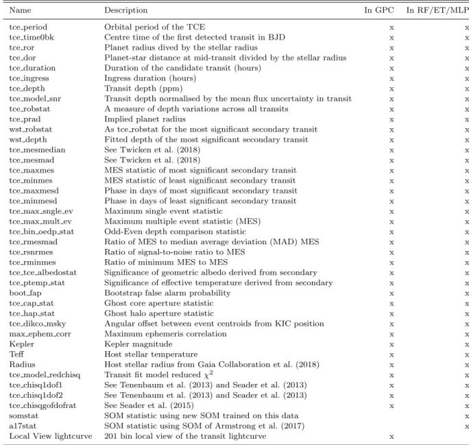
The full range of included data is shown in Table 1. This is a subset of the original TCE table, with several columns
removed based on their contribution to the models as de-scribed in Section 3.3. Brief descriptions of each column are given, readers should refer to the NASA Exoplanet Archive for further detail.
3.2 Lightcurves
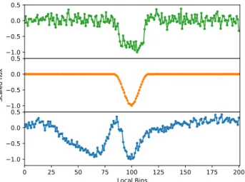
We use the DV Kepler lightcurves, as detailed in Twicken et al. (2018), which are produced in the same way as lightcurves used for the Kepler Transiting Planet Search (TPS). The lightcurve data is phasefolded at the TCE ephemeris then binned into 201 equal width bins in phase covering a region of seven transit durations centred on the candidate transit. We choose these parameters following Shallue & Vanderburg (2018), their ‘local’ view, although we use a window covering one less transit duration to pro-vide better resolution of the transit event. Example local views are shown in Figure 1. Empty bins are filled by in-terpolating surrounding bins. As in Shallue & Vanderburg (2018) we also implemented a ‘global’ view using 2001 phase bins covering the entire phase-folded lightcurve, but in our case found no improvement in classifier performance and so dropped this view to reduce the input feature space. We hypothesise that this is due to the inclusion of additional metrics measuring the significance of secondary eclipses.
We consider several machine learning algorithms in Sec-tion 4. Some algorithms are unlikely to deal well with direct lightcurve data, as it would dominate the feature space. For these we create a summary statistic for the lightcurves fol-lowing the self-organising-map (SOM) method of Armstrong et al. (2017), applying our lightcurves to their publicly avail-ableKepler SOM. We create a further SOM statistic using the same methodology but with a SOM trained on our own dataset, to encourage discrimination of non-astrophysical FPs which weren’t studied in Armstrong et al. (2017). The resulting SOM is shown in Figure 2. These SOM statis-tics are a form of dimensionality reduction, reducing the lightcurve shape into a single statistic.
For a given algorithm, either the two SOM statistics are appended to the TCE table feature set, or the ‘local’ view lightcurve with 201 bin values is appended. As such we have two data representations, ‘Feature+SOM’ and ‘Fea-ture+LC’. The used features, and which models they apply to, are detailed in Table 1.
3.3 Minimally useful attributes
It is desirable to reduce the feature space to the minimum useful set, so as to simplify the resulting model and re-duce the proportion of non-informative features passed to the models. We drop columns from the TCE table using a number of criteria. Initially metadata associated with the table is dropped, including delivery name andKepler iden-tifier. Columns associated with the error on another column are dropped. Columns associated with a trapezoid fit to the lightcurves are dropped in favour of the actual planet model fit also performed. We drop most centroid information, lim-iting the models to one column providing the angular offset between event centroids and the KIC position, finding that this performed better than differential measures. Columns related to the autovetter (McCauliff et al. 2015) are dropped,
1.0 0.5 0.0 0.5 1.0 0.5 0.0 0.5 Scaled flux 0 25 50 75 100 125 150 175 200 Local Bins 1.0 0.5 0.0 0.5
Figure 1.‘Local view’ 201 bin representation of the transit for a planet (top), astrophysical FP (middle) and non-astrophysical FP (bottom).
0.0 2.5 5.0 7.5 10.0 12.5 15.0 17.5 20.0
SOM Pixel Index (x)
0.0 2.5 5.0 7.5 10.0 12.5 15.0 17.5 20.0SOM Pixel Index (y)
Figure 2.SOM pixel locations of labelled training set lightcurves, showing strong clustering. Green=planet, orange = astrophysical FP, blue=non-astrophysical FP. A random jitter of between -0.5 and 0.5 pixels has been added in both axes for clarity.
along with limb darkening coefficients, and the planet albedo and implied temperature are dropped in favour of their as-sociated statistics which better represent the relevant infor-mation for planet validation. We further experimented with removing the remaining features in order to create a mini-mal set, finding that the results in fact marginally improved when we reduced the data table to the thirty eight features detailed in Table 1, in addition to the SOM features or the local view lightcurve.
3.4 Data Scaling
Many machine learning algorithms perform better when the input data is scaled. As such we scale each of our inputs to follow a normal distribution with a mean of zero and vari-ance of unity for each feature. The only exceptions are the ‘local’ view lightcurve values, which are already scaled. The most important four feature distributions as measured by
0.00 0.25 0.50 0.75
1.00
som stat
a17 stat
5.0 2.5 0.0 2.5 5.0 0.00 0.25 0.50 0.75 1.00
Scaled Feature
Density
core aperture
5.0 2.5 0.0 2.5 5.0
centroid offset
Figure 3.Training set distributions of the most important four features after scaling. Confirmed planets are in green, astrophys-ical FPs in orange, and non-astrophysastrophys-ical FPs in blue. The single value peaks occur due to large numbers of TCEs having identical values for a feature. The vertical axis cuts off some of the distribu-tion in the top two panels to better show the overall distribudistribu-tions.
the optimised random forest classifier (RFC) from Section 4 are plotted in Figure 3.4 after scaling.
3.5 Training Set Dispositions
Information on the disposition of each TCE is extracted from the DR25 ordinary and supplementary KOI tables (hereafter koi-base and koi-supp respectively). koi-base is the KOI table derived exclusively from DR25, whereas koi-supp contains a ‘best-knowledge’ disposition for each KOI. We build our confirmed planet training set by taking ob-jects labelled as confirmed in the koi-supp table (column ‘koi disposition’), which are in the koi-base table and not labelled as FPs or indeterminate in either Santerne et al. (2016) or Burke et al. (2019). This set includes previously validated planets. We remove a small number of apparently confirmed planets where theKeplerdata has shown them to be FPs, based on the ‘koi pdisposition’ column. We use koi-supp to give the most accurate dispositions for individual ob-jects, prioritising training set label accuracy over uniformly processed dispositions. This leaves 2274 TCEs labelled as confirmed planets.
We build two FP sets, one each for astrophysical and non-astrophysical FPs. The astrophysical FP set contains all KOIs labelled false positive in the koi-supp table (column ‘koi pdisposition’), which are in the koi-base table, where there is not a flag raised indicating a non-transiting-like sig-nal, and supplemented by all false positives in Santerne et al. (2016). The non-astrophysical FP set contains KOIs where a flag was raised indicating a non-transiting-like signal, sup-plemented by 2200 randomly drawn TCEs which were not upgraded to KOIs. By utilising these random TCEs we are implicitly assuming that the TCEs which were not made KOIs are in the majority FPs, which is born out by our re-sults (Section 6.2). The astrophysical FP set then has 3100 TCEs, and the non-astrophysical FP set has 2959 TCEs.
Table 1.Data features. GPC=Gaussian Process Classifier, RF=Random Forest, ET=Extra Trees, MLP=Multilayer Perceptron.
Name Description In GPC In RF/ET/MLP
tce period Orbital period of the TCE x x
tce time0bk Centre time of the first detected transit in BJD x x
tce ror Planet radius dived by the stellar radius x x
tce dor Planet-star distance at mid-transit divided by the stellar radius x x
tce duration Duration of the candidate transit (hours) x x
tce ingress Ingress duration (hours) x x
tce depth Transit depth (ppm) x x
tce model snr Transit depth normalised by the mean flux uncertainty in transit x x tce robstat A measure of depth variations across all transits x x
tce prad Implied planet radius x x
wst robstat As tce robstat for the most significant secondary transit x x wst depth Fitted depth of the most significant secondary transit x x
tce mesmedian See Twicken et al. (2018) x x
tce mesmad See Twicken et al. (2018) x x
tce maxmes MES statistic of most significant secondary transit x x tce minmes MES statistic of least significant secondary transit x x tce maxmesd Phase in days of most significant secondary transit x x tce minmesd Phase in days of least significant secondary transit x x
tce max sngle ev Maximum single event statistic x x
tce max mult ev Maximum multiple event statistic (MES) x x
tce bin oedp stat Odd-Even depth comparison statistic x x
tce rmesmad Ratio of MES to median average deviation (MAD) MES x x
tce rsnrmes Ratio of signal-to-noise ratio to MES x x
tce rminmes Ratio of minimum MES to MES x x
tce tce albedostat Significance of geometric albedo derived from secondary x x tce ptemp stat Significance of effective temperature derived from secondary x x
boot fap Bootstrap false alarm probability x x
tce cap stat Ghost core aperture statistic x x
tce hap stat Ghost halo aperture statistic x x
tce dikco msky Angular offset between event centroids from KIC position x x
max ephem corr Maximum ephemeris correlation x x
Kepler Kepler magnitude x x
Teff Host stellar temperature x x
Radius Host stellar radius from Gaia Collaboration et al. (2018) x x
tce model redchisq Transit fit model reducedχ2 x x
tce chisq1dof1 See Tenenbaum et al. (2013) and Seader et al. (2013) x x tce chisq1dof2 See Tenenbaum et al. (2013) and Seader et al. (2013) x x
tce chisqgofdofrat See Seader et al. (2015) x x
somstat SOM statistic using new SOM trained on this data x
a17stat SOM statistic using SOM of Armstrong et al. (2017) x
Local View lightcurve 201 bin local view of the transit lightcurve x
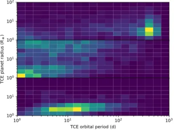
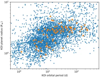
The planet radius and period distributions of the three sets are shown in Figure 3.5.
We combine the two FP sets going forwards, leaving a FP set with approximately double the number of the con-firmed planet set. This imbalance will be corrected implicitly by some of our models, but in cases where it isn’t, or in case the correction is not effective, this overabundance of FPs en-sures that any bias in the models prefers FP classifications. We do not include additional TCEs to avoid unbalancing the training sets further, which can impact model performance.
We split our data into a training set (80%, 6663 TCEs), a validation set for model selection and optimisation (10%, 834 TCEs) and a test set for final analysis of model per-formance (10%, 836 TCEs), in each case maintaining the proportions of planets to FPs. TCEs with no disposition form the ’unknown’ set (24201 TCEs).
3.6 Training Set Scenario Distributions
The algorithms we are building fundamentally aim to derive the probability that a given input is a member of one of the given training sets. As such the membership, information in, and distributions of the training sets are crucially im-portant. The overall proportion of FPs relative to planets is deliberately left to be incorporated as prior information. We could attempt to include it by changing the relative numbers within the confirmed planet and FP datasets, but the num-ber of objects in a training set is not trivially related to the output probability for most machine learning algorithms.
Another consideration is the relative distributions of ob-ject parameters within each of the planet and FP datasets. This is where the effect of, for example, planet radius on the likelihood of a given TCE being a FP will appear. By taking the confirmed and FP classifications of the koi-supp table as our input, we are implicitly building in any biases present in that table into our algorithm. We note that the table
100 101 102 100 101 TC E pla ne t r ad ius (R ) 100 101 102 103
TCE orbital period (d)
100
101
Figure 4. Training set planet radius and period distributions. Top: Non-astrophysical FPs. Middle: Astrophysical FPs. Bottom: planets. All distributions are normalised to show probability den-sity. Training set members with apparent planet radii larger than 100R⊕are not plotted for clarity (all are FPs).
distribution is in part the real distribution of planets and FPs detected by theKeplersatellite and the detection algo-rithms which created the TCE and KOI lists. Incorporating that distribution is in fact desirable, given we are studying candidates found using the same process, and in that sense the Kepler set of planets and FPs is the ideal distribution to use.
The distribution of Kepler detected planets and FPs we use will however be biased by the methods used to la-bel KOIs as planets and FPs. In particular the majority of confirmed planets and many FPs labelled in the KOI list have been validated by the vespa algorithm (∼50% of the known KOI planets), and as such biases in that algorithm may be present in our results. We compare our results to the
vespadesignations in Section 6.5, showing they disagree in many cases despite this reliance onvespadesignations. The reliance on past classification of objects as planet or FP is a weakness of our method which we aim to improve in future work, using simulated candidates from each scenario.
A further point is the balance of astrophysical to non-astrophysical FPs in the training set. We can estimate what this should be using the ratio of KOIs to TCEs, where KOIs are ∼30% of the TCE list, under the assumption that the
majority of non-KOI TCEs are non-astrophysical FPs. We use a 50% ratio in our training set, which effectively in-creases the weighting for the astrophysical FPs. This ratio improves the representation of astrophysical FPs, which is desirable given that non-astrophysical FPs are easy to dis-tinguish given a high enough signal-to-noise. We impose a MES cut of 10.5 as recommended by Burke et al. (2019) be-fore validating any candidate to remove the possibility of low signal-to-noise instrumental FPs complicating our results.
4 MODEL SELECTION AND OPTIMISATION
Many machine learning methods are available, with a range of complexity and properties. We perform empirical model
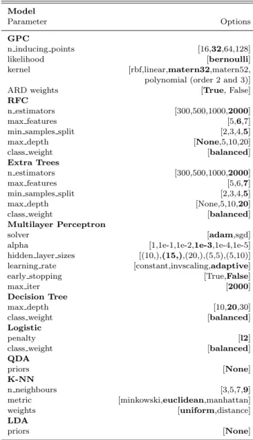
selection using the two input data sets. For the Fea-ture+SOM set, we implement eight models with a range of parameters, testing a total of 822 combinations, using the
scikit-learn pythonmodule (Pedregosa et al. 2011). The best parameters for each algorithm were selected by compar-ing scores on the validation set. The trialled model param-eters are shown in Table 2, with the best found paramparam-eters highlighted. The final performances of each model are given in Table 3, with and without probability calibration which is described in Section 5.1, and are measured using the log-loss metric (see e.g. Malz et al. 2019) calculated on the test set. The log-loss is given by
Llog=− 1 N N−1 X i=0 (yilog(pi) + (1−yi) log(1−pi)) (5)
whereyi is the true class label of candidate iand pi is its
output classifier score, andN is the number of test samples. The utilised models are described in Section 2, but readers interested in the other models are referred to the
scikit-learn documentation and references therein (Pe-dregosa et al. 2011).
We found that while most tested models were highly successful, the best performance after calibration was shown by a RFC. It is interesting to see the relative success of even very simple models such as Linear Discriminant Anal-ysis (LDA), implying the underlying decision space is not overly complex. The overall success of the models is not un-expected, as we are providing the classifiers with very similar information as was often used to classify candidates as plan-ets or FPs in the first place, and in the case ofvespa vali-dated candidates, we are adding more detailed lightcurve in-formation. We proceed with the RFC as a versatile robust al-gorithm, supplementing the results with classifications from the next two most successful models, Extra Trees (ET) and Multi-layer Perceptron (MLP), to guard against overfitting by any one model.
For the Feature+LC input data, we utilise a gaussian process classifier (GPC) to provide an independent and nat-urally probabilistic method for comparison and to guard against overconfidence in model classifications. We imple-ment the GPC usinggpflow. The GPC is optimised varying the selected kernel function, and final performance is shown in Table 3. Additionally we trial the GPC using variations of the input data - with the Feature+SOM data, lightcurve and a subset of features (Features+LC-light) and with the full Feature+LC dataset. We find the results are not strongly dependent on input dataset, and hence use the Feature+LC dataset to provide a difference to the other models. Figure 4 shows the GPC adapting to the input transit data. The underlying theory of a GPC was summarised in Section 2.2.
5 PLANET VALIDATION
5.1 Probability Calibration
Although the GPC naturally produces probabilities as out-putp(s = 1| x∗), the other classifiers are inherently non-probabilistic models and need to have their ad-hoc proba-bilities calibrated (Zadrozny & Elkan 2001, 2002; Niculescu-Mizil & Caruana 2005). Classifier probability calibration is typically performed by plotting the ‘calibration curve’, the
1.0 0.5 0.0 0.5 Scaled flux 0 25 50 75 100 125 150 175 200 Local Bins 5 10 15 20 GPC length scale
Figure 5.Top: Local view of a planet lightcurve. Bottom: GPC automatic relevance determination (ARD) lengthscales for each of the input bins in the local view. Low lengthscales can be seen at ingress and egress, demonstrating that the GPC has learned to prioritise those regions of the lightcurve when making classifi-cations.
fraction of class members as a function of classifier output. The uncalibrated curve is shown in Figure 5.1, which high-lights a counterintuitive issue; the better a classifier per-forms, the harder it can be to calibrate, due to a lack of objects being assigned intermediate values. Given our focus is to validate planets, we focus on accurate and precise cal-ibration at the extreme ends, wherep(s= 1|x∗)<0.01 or
p(s= 1|x∗)>0.99.
To statistically validate a candidate as a planet, the commonly accepted threshold isp(s= 1|x∗)>0.99 (Morton et al. 2016). Measuring probabilities to this level requires the precision of our calibration is also at least 1% or better. We use theisotonic regression calibration technique (Zadrozny & Elkan 2001, 2002), which calibrates by counting samples in bins of given classifier scores. To measure the fraction of true planets in thep(s = 1|x∗)>0.99 bin we therefore re-quire at leastN = 10000 test planets to reduce the Poisson counting error√N /Nbelow 1%. Given the size of our train-ing set additional test inputs are required for calibration.
To allow calibration at this precision, we synthesise ad-ditional examples of planets and FPs from our training set, by interpolating between members of each class. The process is only performed for the Feature+SOM dataset, as the GPC does not need calibrating. We select a training set member at random, and then select another member of the same class which is within the 20th percentile of all the member-to-member distances within that class. Distances are cal-culated by considering the euclidean distance between the values of each column for two class members. Restricting the distances in this way allows for non-trivial class bound-aries in the parameter space. A new synthetic class member is then produced by interpolating between the two selected real inputs. We generate 10000 each of planets and FPs from the training set. These synthetic datasets are used only for calibration, not to train the classifiers.
It is important to note that by interpolating, we have es-sentially weakened the effect of outliers in the training data, at least for the calibration step. For this and other reasons,
Table 2.Trialled model parameters. All combinations listed were tested. Best parameters as found on the validation set are in bold.
Model
Parameter Options
GPC
n inducing points [16,32,64,128]
likelihood [bernoulli]
kernel [rbf,linear,matern32,matern52, polynomial (order 2 and 3)]
ARD weights [True, False]
RFC
n estimators [300,500,1000,2000]
max features [5,6,7]
min samples split [2,3,4,5]
max depth [None,5,10,20]
class weight [balanced]
Extra Trees
n estimators [300,500,1000,2000]
max features [5,6,7]
min samples split [2,3,4,5]
max depth [None,5,10,20]
class weight [balanced]
Multilayer Perceptron
solver [adam,sgd]
alpha [1,1e-1,1e-2,1e-3,1e-4,1e-5] hidden layer sizes [(10,),(15,),(20,),(5,5),(5,10)] learning rate [constant,invscaling,adaptive]
early stopping [True,False]
max iter [2000]
Decision Tree
max depth [10,20,30]
class weight [balanced]
Logistic
penalty [l2]
class weight [balanced]
QDA
priors [None]
K-NN
n neighbours [3,5,7,9]
metric [minkowski,euclidean,manhattan]
weights [uniform,distance]
LDA
priors [None]
candidates which are outliers to our training set will not get valid classifications, and should be ignored. We describe our process for flagging outliers in Section 5.5. Interpolation also means that while we can attain the desired precision, the ac-curacy of the calibration may still be subject to systematic biases in the training set, which were discussed in Section 3.6.
5.2 Classifier training
The GPC was trained using the training data with no cal-ibration. We used thegpflow(de G Matthews et al. 2017)
python extension totensorflow (Abadi et al. 2016), run-ning on an NVidia GeForce GTX Titan XP GPU. On this architecture the GPC takes less than one minute to train, and seconds to classify new candidates.
For the other classifiers, training and calibration was performed on a 2017 generation iMac with four 4.2GHz In-tel i7 processors. Training each model takes a few minutes,
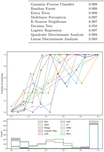
Table 3.Best model performance on test set, ranked by calibrated log-loss. The GPC does not require external calibration. Model AUC Precision Recall Log-loss Calibrated Log-loss Gaussian Process Classifier 0.999 0.984 0.995 0.54 —
Random Forest 0.999 0.981 0.997 0.58 0.54 Extra Trees 0.999 0.985 0.992 0.58 0.58 Multilayer Perceptron 0.997 0.982 0.985 0.83 0.66 K-Nearest Neighbours 0.997 0.995 0.972 0.83 0.66 Decision Tree 0.958 0.979 0.984 0.95 0.74 Logistic Regression 0.997 0.988 0.967 1.12 1.03
Quadratic Discriminant Analysis 0.989 0.983 0.970 1.16 1.20 Linear Discriminant Analysis 0.993 0.982 0.965 1.32 1.36
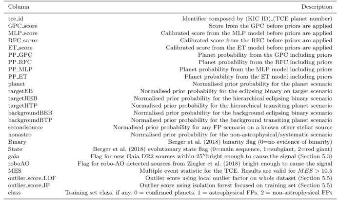
0.0 0.2 0.4 0.6 0.8 1.0 0.0 0.2 0.4 0.6 0.8 1.0 Fraction of positives 0.0 0.2 0.4 0.6 0.8 1.0
Mean predicted value 0 100 200 300 400 500 600 Count RFC QDA Ridge Logistic Reg LDA SVC ET KNN DT MLP
Figure 6.Top: Calibration curve for the uncalibrated non-GP classifiers. The black dashed line represents perfect calibration. Bottom: Histogram of classifications showing the number of can-didates falling in each bin for each classifier.
with classification of new objects possible in seconds. To cre-ate calibrcre-ated versions of the other classifiers, we employ a cross validation strategy to ensure that the training data can be used for training and calibration. The training set and synthetic dataset are split into 10 folds, and on each iteration a classifier is trained on 90% of the training data, then calibrated on the remaining 10% of training data plus 10% of the synthetic data. The process is repeated for each fold to create ten separate classifiers, with the classifier re-sults averaged to produce final classifications.
The above steps suffice to give results on the valida-tion, test and unknown datasets. We also aim to classify the training dataset independently, as a sanity check and to confirm previous validations. To get results for the train-ing dataset we introduce a further layer of cross-validation, with 20 folds. For the GPC this is the only cross validation, where the GPC is trained on 95% of the training data to give a result for the remaining 5%, and the process repeated to classify the whole training set. For the other classifiers we separate 5% of the training data before performing the above
0.0 0.2 0.4 0.6 0.8 1.0 0.0 0.2 0.4 0.6 0.8 1.0 Fraction of positives 0.0 0.2 0.4 0.6 0.8 1.0
Mean predicted value 0 2000 4000 6000 8000 10000 12000 14000 Count RFC QDA Logistic Reg LDA ET KNN DT MLP 0.000 0.005 0.010 0.015 0.020 0.00 0.01 0.02 0.980 0.985 0.990 0.995 1.000 0.98 0.99 1.00
Figure 7.Top: Calibration curve for the calibrated non-GP clas-sifiers. The black dashed line represents perfect calibration. The two insets show zoomed plots of the low and high ends of the curve. Bottom: Histogram of classifications showing the number of candidates falling in each bin for each classifier. Synthetic train-ing set members are included in this plot.
training and calibration steps using the remaining 95%, and repeat.
5.3 Positional Probabilities
Part of the prior probability for an object to be a planet or FP,P(s|I), is the probability that the signal arises from the target star, a known blended star in the aperture, or an unresolved background star. We derive these values using the positional probabilities calculated in Bryson & Morton (2017), which provide the probability that the signal arises from the target star Ptarget, the probability arises from a
known secondary sourcePsecondsource, typically another KIC
target or a star in theKeplerUKIRT survey1, and the prob-ability the signal arises from an unresolved background star
Pbackground. Bryson & Morton (2017) also considered a small
number of sources detected through high resolution imag-ing; we ignore these and instead take the most up to date results from the robo-AO survey from Ziegler et al. (2018). The given positional probabilities have an associated score representing the quality of the determination; where this is below the accepted threshold of 0.3 we continue with the a priori values given by Bryson & Morton (2017), but do not validate planets where this occurs.
The calculation in Bryson & Morton (2017) was per-formed without Gaia DR2 (Gaia Collaboration et al. 2018) information, and so we update the positional probabilities using the new available information. We first search the Gaia DR2 database for any detected sources within 2500of each TCE host star. We chose 2500as this is the limit considered for contaminating background sources in Bryson & Mor-ton (2017). Gaia sources which are in the KIC (identified in Berger et al. 2018), in the Kepler UKIRT survey or in the new robo-AO companion source list are discarded as these were either accounted for in Bryson & Morton (2017) or are considered separately in the case of robo-AO.
We then check for each TCE whether any new Gaia or robo-AO sources are bright enough to cause the ob-served signal, conservatively assuming a total eclipse of the blended background source. If there are such sources, we flag the TCE in our results and adjust the probability of a background source causing the signal Pbackground to
ac-count for the extra source, by increasing the local density of unresolved background stars appropriately and normal-ising the set of positional probabilities given the new value ofPbackground. It would be ideal to treat the Gaia source as
a known second source, but without access to the centroid ellipses for each candidate we cannot make that calculation. We do not validate TCEs with a flag raised for a detected Gaia or robo-AO companion, although we still provide re-sults in Section 6.
5.4 Prior Probabilities
To satisfy Equation 1 we need the prior probability of a given candidate being a planet or FP,P(s|I), independently of the candidate parameters. This prior probability for the planet scenario is given by
P(s= 1|I) =Ptargetfplanetftransit (6)
where Ptarget is the probability of a signal arising from the
host star and was calculated in Section 5.3, fplanet is the
probability of a randomly chosen star hosting a planet that
Kepler could detect and ftransit represents the probability
of that planet transiting, on average over the Kepler can-didate distribution. The product fplanetftransit represents
the probability that a randomly chosenKepler target star hosts a planet which could have been detected by the Ke-pler pipeline. We derive the productfplanetftransitusing the
occurrence rates calculated by Hsu et al. (2018), for planets with periods less than 320d and radii between 2 and 12R⊕.
We take each occurrence rate bin in their paper, calculate the eclipse probability for a planet in the centre of the bin to transit a solar host star, and sum the resulting probabilities to get a final productfplanetftransit = 0.0308. The effect of
specific planet radius, period and host star is included in the classification models.
We consider several FP scenarios and sum their proba-bilities to give the overall prior for FPs. We take
P(s= 0|I) =P(FP-EB) +P(FP-HEB) +P(FP-HTP) +P(FPresolved) +P(FP-BEB) +P(FP-BTP) +P(FPnon-astro) (7)
where P(FP-EB) is the prior for an eclipsing binary on the target star,P(FP-HEB) is the prior for a hierarchical eclipsing binary, i.e. a triple system where the target star has an eclipsing binary companion causing the signal, and
P(FP-HTP) is the prior for a hierarchical transiting planet, i.e. a planet transiting the fainter companion in a binary system.P(FPresolved) is the prior for a transiting planet, eclipsing binary or hierarchical eclipsing binary on a resolved non-target star. We disregard hierarchical transiting planets on second known sources as contributing insignificantly to-wards the FP probability.P(FP-BEB) andP(FP-BTP) are the priors for an eclipsing binary or a transiting planet on an unresolved background star.P(FPnon-astro) is the prior for an instrumental or otherwise non-astrophysical source of the signal. We do not consider planets transiting the target star to be FPs even in the case where other stars, bound or otherwise, are diluting the signal. In our methodology these priors are independent of the actual orbital period of the contaminating binary, and so TCE FPs where the FP is an eclipsing binary with half the actual binary orbital period, as seen in Morton et al. (e.g. 2016), are covered by the same priors.
For the scenario specific priors,
P(FP-EB) =Ptargetfclose-binaryfeclipse (8)
P(FP-HEB) =Ptargetfclose-triplefeclipse (9)
P(FP-HTP) =Ptargetfbinaryfplanetftransit (10)
P(FPresolved) =Psecondsource(fclose-binaryfeclipse+ fclose-triplefeclipse+fplanetftransit) (11)
P(FP-BEB) =Pbackground(fclose-binaryfeclipse) (12)
P(FP-BTP) =Pbackground(fplanetftransit) (13)
wherePtarget,PsecondsourceandPbackgroundwere derived
in Section 5.3. We discuss each prior in turn.
5.4.1 P(FP-EB)
To calculate P(FP-EB) we need the probability of a ran-domly chosen star being an eclipsing binary with an orbital
periodPwhichKepler could detect. We calculate the prod-uctfclose-binaryfeclipse using the results of Moe & Di Stefano
(2017). We integrate their occurrence rate for companion stars to main sequence solar-like hosts as a function of logP
(their equation 23) multiplied by the eclipse probability at that period for a solar host star. We consider companions with logP <2.5 (P <320d) and mass ratio q >0.1, cor-recting from the q > 0.3 equation using a factor of 1.3 as suggested. The integration givesfclose-binaryfeclipse= 0.0048,
which is strikingly lower than the planet prior, primarily due to the much lower occurrence rate for close binaries. Ignor-ing eclipse probability, we find the frequency of solar-like stars with companions within 320d to be 0.055 from Moe & Di Stefano (2017). It is often stated that∼50% of stars are in multiple systems, but this fraction is dominated by wide companions with orbital periods longer than 320d. This cal-culation implicitly assumes that any eclipsing binary in this period range with mass ratio greater than 0.1 would lead to a detectable eclipse in theKeplerdata.
5.4.2 P(FP-HEB)
The probability that a star is a hierarchical eclipsing binary depends on the triple star fraction. In our context the prod-uct fclose-triplefeclipse is the probability for a star to be in
a triple system, where the close binary component is in the background, has an orbital period short enough forKeplerto detect, and eclipses. The statistics for triple systems of this type (A-(Ba,Bb)) are extremely poor (Moe & Di Stefano 2017) due to the difficulty of reliably detecting additional companions to already lower mass companion stars. If we assume that one of the B components is near solar-mass, then we can use the general close companion frequency, which is the same asfclose-binaryfeclipse, multiplied by an
ad-ditional factor to account for an adad-ditional wider compan-ion. We use the fraction of stars with any companion from Moe & Di Stefano (2017), which isfmultiple= 0.48. As such
we takefclose-triplefeclipse=fmultiplefclose-binaryfeclipse. Again
this calculation implicitly assumes that any such triple with mass ratios greater than 0.1 to the primary star would lead to a detectable eclipse in theKepler data.
5.4.3 P(FP-HTP)
Unlike the stellar multiple cases it is unlikely that all back-ground transiting planets would produce a detectable sig-nal in the Kepler data. Estimating the fraction that do is complex and would require an estimate of the transit depth distribution for the full set of background transiting planets. Instead we proceed with the assumption that all such plan-ets would produce a detectable signal if in a binary system, but not in systems of higher order multiplicity.fbinary= 0.27
from Moe & Di Stefano (2017) for solar-like primary compo-nents, which is largely informed by Raghavan et al. (2010).
fplanetftransit= 0.0308 as calculated above. Note we do not
include any effect of multiplicity on the planet occurrence rate.
All necessary components for the remaining priors have now been discussed, although we again note the implicit assumption that all scenarios could produce a detectable transit.
5.4.4 P(FPnon-astro)
P(FPnon-astro) is difficult to calculate, and so we follow Morton et al. (2016) in setting it to 5e-5. Recent work has suggested that the systematic false alarm rate is highly im-portant when considering long period small planetary can-didates (Burke et al. 2019) and can be the most likely source of FPs for such candidates. The low prior rate for non-astrophysical FPs used here is justified because we apply a cut on the multiple event statistic (MES) of 10.5 as rec-ommended by Burke et al. (2019), allowing only significant candidates to be validated. At such an MES, the ratio of the systematic to planet prior is less than 10−3(Burke et al. 2019, their Figure 3), which translates to a prior of order 10−5 when applied to our planet scenario prior.
5.4.5 Prior information in the training set
Note that the probability of the signal arising from the tar-get star is included in our scenario prior asPtarget. As some
centroid information is included in the training data the classifiers may incorporate the probability of the signal aris-ing from the target star internally. As such we are at risk of double counting this information in our posterior probabil-ities. We include positional probabilities inP(s|I) because the probabilities available from Bryson & Morton (2017) include information on nearby stars and their compatibil-ity with the centroid ellipses derived for each TCE. This is more information than we can easily make available to the classifiers, and additionally improves interpretability by exposing the positional probabilities directly in the calcu-lation. Removing centroid information from the classifiers would artificially reduce their performance. Including prior information on the target in both the classifiers and exter-nal prior is the conservative approach, because a significant centroid offset, or low target star positional probability, can only reduce the derived probability of a TCE being a planet.
5.5 Outlier Testing
Our method is only valid for ‘inliers’, candidates which are well represented by the training set and which are not rare or unusual. We perform two tests to flag outlier TCEs, using different methodologies for independence.
The first considers outliers from the entire set of TCEs, to avoid mistakenly validating a candidate which is a unique case and hence might be misinterpreted. We implement the local outlier factor method (Breunig et al. 2000), which mea-sures the local density of an entry in the dataset with respect to its neighbours. The result is a factor which decreases as the local density drops. If that factor is particularly low, the entry is flagged as an outlier. We use a default threshold of -1.5 which labels 391 (1.2%) of TCEs as outliers, 108 of which were KOIs. The local outlier factor is well suited to studying the whole dataset as it is an unsupervised method which requires no separate training set.
The second outlier detection method aims to find ob-jects which are not well represented in the training set specif-ically. In this case we implement an isolation forest (Liu et al. 2008) with 500 trees, which is trained on the training set then applied to the remaining data. Figure 5.5 shows
0.60 0.55 0.50 0.45 0.40 0 200 400 600 800 1000 N Isolation Forest 1.8 1.7 1.6 1.5 1.4 1.3 1.2 1.1 1.0 0.9 Outlier Score 0 1000 2000 3000 N
Local Outlier Factor
Figure 8.Top: Isolation Forest outlier score for all TCEs in blue and KOIs in orange. The red dashed line represents the threshold for outlier flagging. Bottom: As top for Local Outlier Factor. In both case outliers have more negative scores.
the distribution of scores produced from the isolation for-est, where lower scores indicate outliers. The majority of candidates show a normal distribution, with a tail of more outlying candidates. We set our threshold as -0.55 based on this distribution, which flags 1979 (6.1%) of TCEs as out-liers, 932 of which were KOIs.
5.6 External Flags
Some information is only available for a small fraction of the sample, and hence is hard to include directly in the models. In these cases, we create external flags along with our model scores, and conservatively withhold validation from planets where a warning flag is raised.
As described in Section 5.3, we flag TCEs where either Gaia DR2 or Robo-AO has detected a previously unresolved companion in the aperture bright enough to cause the ob-served TCE. The robo-AO flag supersedes the Gaia flag, in that if a source is seen in robo-AO we will not raise the Gaia flag for the same source. We also flag TCEs where the host star has been shown to be evolved in Berger et al. (2018) us-ing the Gaia DR2 data, and include the Berger et al. (2018) binarity flag which indicates evidence for a binary compan-ion from either the Gaia parallax or alternate high resolutcompan-ion imaging.
5.7 Training Set Coverage
It is crucial to be aware of the content of our training set: planet types or FP scenarios which are not represented will not be well distinguished by the models. The training set here is drawn from the real detected Kepler distribution of planets and FPs, but potential biases exist for situations which are hard to disposition confidently. For example, small planets at low signal to noise will typically remain as candi-dates rather than being confirmed or validated, and certain difficult FP scenarios such as transiting brown dwarfs are un-likely to be routinely recognised. In each case, such objects are likely to be more heavily represented in the unknown, non-dispositioned set.
For planets, we have good coverage of the planet set as a whole, as this is the entire confirmed planet training set, but planets in regions of parameter space whereKeplerhas poor sensitivity should be viewed with suspicion.
For FPs, our training set includes a large number of non-astrophysical TCEs, giving good coverage of that scenario. For astrophysical FPs, we first make sure our training set is as representative as possible by including externally flagged FPs from Santerne et al. (2016). These cases use additional spectroscopic observations to mark candidates as FPs. How-ever the bulk of smallKeplercandidates are not amenable to spectroscopic followup due to their stellar brightness. Utilis-ing the FP flags in the archive as an indicator of the FP sce-nario, we have 2147 FPs showing evidence of stellar eclipses, and 1779 showing evidence of centroid offset and hence back-ground eclipsing sources. 1087 show ephemeris matches, an indicator of a visible secondary eclipse and hence a stellar source. As such we have a wide coverage of key FP scenarios. It would be ideal to probe scenario by scenario and test the models in this fashion. Future work using specific sim-ulated datasets will be able to explore this in more detail. Rare and difficult scenarios such as background transiting planets and transiting brown dwarfs are likely to be poorly distinguished by our or indeed any comparable method. In rare cases such as background transiting planets, which typ-ically have transits too shallow to be detected, the effect on our overall results will be minimal. We note that these issues are equally present for currently utilised validation methods, andvespafor example cannot distinguish transiting brown dwarfs from planets (Morton et al. 2016).
6 RESULTS
Our classification results are given in Table 4. The Table contains the classifier outputs for each TCE, calibrated if appropriate, as well as the relevant priors and final posterior probabilities adjusted by the priors. Several warning flags are included representing outliers, evolved host stars and detected close companions. Table A1 shows the subset of Table 4 for KOIs, and includes KOI specific information and
vespaprobabilitiies calculated for DR25.
6.1 Previously dispositioned objects
To sanity check our method we consider the results of al-ready dispositioned TCEs. For this testing we focus on the GPC results. There are two planets in the confirmed train-ing set which score<0.01 in the GPC after applying the prior information. These are KOI2708.01 and KOI00697.01. Despite being labelled as confirmed in the NASA Exoplanet Archive KOI2708.01 is actually a certified FP, due a high level period match. This status is reflected in the positional probabilities, which give a relative probability of zero that the TCE originates from the host star. KOI00697.01 also has a positional probability indicating that the transit ac-tually arises from a background star with high confidence,
>0.9999. It is clear that both KOIs should be labelled FP. There is also one KOI labelled as a FP which gains a score of>0.99 in the GPC, KOI3226.01. This KOI has a flag raised for having a ‘not-transit-like’ signal. Visual inspection of the KOI shows stellar variability on a similar level to the
[h]
Table 4.Full data table available online. This table describes the available columns.
Column Description
tce id Identifier composed by (KIC ID) (TCE planet number)
GPC score Score from the GPC before priors are applied
MLP score Calibrated score from the MLP model before priors are applied RFC score Calibrated score from the RFC before priors are applied ET score Calibrated score from the ET model before priors are applied
PP GPC Planet probability from the GPC including priors
PP RFC Planet probability from the RFC including priors
PP MLP Planet probability from the MLP model including priors
PP ET Planet probability from the ET model including priors
planet Normalised prior probability for the planet scenario
targetEB Normalised prior probability for the eclipsing binary on target scenario targetHEB Normalised prior probability for the hierarchical eclipsing binary scenario targetHTP Normalised prior probability for the hierarchical transiting planet scenario backgroundBEB Normalised prior probability for the background eclipsing binary scenario backgroundBTP Normalised prior probability for the background transiting planet scenario secondsource Normalised prior probability for any FP scenario on a known other stellar source nonastro Normalised prior probability for the non-astrophysical/systematic scenario Binary Berger et al. (2018) binarity flag (0=no evidence of binarity) State Berger et al. (2018) evolutionary state flag (0=main sequence, 1=subgiant, 2=red giant) gaia Flag for new Gaia DR2 sources within 2500bright enough to cause the signal (Section 5.3) roboAO Flag for robo-AO detected sources from Ziegler et al. (2018) bright enough to cause the signal MES Multiple event statistic for the TCE. Results are valid forM ES >10.5 outlier score LOF Outlier score using local outlier factor on whole dataset (Section 5.5) outlier score IF Outlier score using isolation forest focused on training set (Section 5.5) class Training set class, if any. 0 = confirmed planets, 1 = astrophysical FPs, 2 = non-astrophysical FPs
transit signal, which may be distorting the transit signal on a quarter-by-quarter basis. The transits are however still evident in the lightcurve, and do not otherwise appear sus-picious. We do not validate KOI03226.01, but our results indicate that its disposition may need to be reconsidered.
6.2 Non-KOI TCEs
We additionally consider high scoring TCEs which are not in the KOI list to see if any merit further consideration. Nine TCEs score>0.99 in the GPC while passing our other checks. In each case the TCE was associated with the sec-ondary eclipse of another TCE. For these TCEs, the Ke-pler transiting planet search found the first TCE which was removed and the lightcurve searched again. In these cases the secondary eclipse of the original TCE remained in the lightcurve, and was ‘discovered’ as an additional TCE. It appears metrics such as secondary eclipse depth were calcu-lated after removing the primary eclipse, and so these ‘sec-ondary’ TCEs give all the indications of being planetary candidates. Such TCEs do not become KOIs and so would not be in danger of being mislabelled as validated planets. They highlight the dangers of poor information, in this case erroneous secondary eclipse measurements, both to our and other validation methods.
Overall the non-KOI TCEs have a mean GPC derived planet probability of 0.018, and a median of 0.002, as ex-pected given these were not considered viable KOIs.
Table 5.GPC scores by KOI radius and multiplicity
Selection Number GPC P Planet
Mean Median
All 7048 0.474 0.379
KOI singles 6148 0.296 0.013
KOIs in multiple systems 1906 0.825 0.994 Rp>= 15R⊕ 1558 0.029 0.006
10R⊕<=Rp<15R⊕ 323 0.295 0.063
4R⊕<=Rp<10R⊕ 824 0.351 0.029
2R⊕<=Rp<4R⊕ 2482 0.666 0.982
Rp<2R⊕ 2867 0.456 0.360
6.3 Dependence on candidate parameters
We investigate our model dependence on candidate param-eters using the KOI list, discounting outliers as described in Section 5.5 but including KOIs with other warning flags. We focus on the planet probability as calculated by the GPC.
Table 5 shows the average planet probability including priors for KOIs based on planet radius and multiplicity, and demonstrates that KOIs in multiple systems score highly as would be expected from past studies of the effect of mul-tiplicity onKepler FP occurrence rates. The high score of KOIs in multiple systems occurs despite no information on multiplicity being passed to the models. Table 5 also shows that the GPC planet probability decreases for giant planets, in agreement with previous studies showing the rate of FPs is larger for giant planet candidates (Santerne et al. 2016). Figure 9 shows the median scores for KOIs of different radii and orbital period.
0.0 0.5 1.0 1.5 2.0 2.5 Log (Orbital Period (d))
0.2 0.0 0.2 0.4 0.6 0.8 1.0 1.2 1.4 Lo g (P lan et R ad ius (R )) 0.0 0.2 0.4 0.6 0.8 1.0 GPC planet probability
Figure 9.Mean GPC planet probability for KOIs binned in log planet radius and orbital period. Bins with no TCEs are white. Giant planets, and those at particularly long or short periods, are more likely to be classed as FPs. The GPC has more confidence in candidates in well-populated regions of parameter space, and loses confidence on average in KOIs which are near the limits of
theKeplersensitivity in the lower right section of the figure.
Table 6.GPC planet probabilities for Santerne et al. (2016) dis-positioned KOIs
Selection Number GPC GPC P Planet Mean Median Planets 44 0.711 0.808 EB 48 0.166 0.100 CEB 15 0.163 0.045 BD 3 0.908 0.910 Unknown 18 0.688 0.717
6.4 Comparison to Santerne et al. (2016)
Santerne et al. (2016) provided dispositions of someKepler
candidates using independent data. The mean and median planet probabilities from the GPC are shown for each dis-position type in Santerne et al. (2016) in Table 6, including planets, brown dwarfs (BD), eclipsing binaries (EB), con-taminating eclipsing binaries (CEB) and unknowns.
We achieve a high score for planets and low scores for EBs and CEBs. BDs are also scored highly, indicating we are insensitive to that FP scenario similarly tovespa (Mor-ton et al. 2016), although in our case the BDs score lower and well below the validation threshold. Typically our model is less confident of giant planets (Table 5) and this guards against the inaccurate validation of brown dwarfs. We hy-pothesis that this is also why the Santerne et al. (2016) plan-ets score relatively lower than the general confirmed planet case, as they are larger than the average KOI.
6.5 Comparison to vespa
Figure 10 shows the GPC scores as compared to the FPP calculated by vespa (Morton et al. 2016). We use the up-dated vespa false positive probabilities (FPPs) available at the NASA Exoplanet Archive for DR25, and consider only
KOIs which pass our outlier checks. The DR25vespa FPP scores have not been published in their own paper and hence have not been used to update planet dispositions in the Ex-oplanet Archive, despite being available there. GPC scores are plotted before application of prior information to allow a more direct comparison, as thevespaprobabilities available on the NASA exoplanet archive appear not to include up-dated positional probability information. Although the plot appears remarkably divergent we highlight that in 73% per-cent of cases the classification is the same using a threshold of 50%. Both methods tend to confidently classify candi-dates as planets or FPs, with intermediate values sparsely populated. Furthermore, candidates which do receive inter-mediate scores show no correlation between the methods. As such we caution against using such intermediate candidates for occurrence rate studies, even if weighting by the GPC score orvespaFPP would appear to be statistically valid.
The methods also strongly disagree in a small but sig-nificant number of cases. Figure 11 shows a zoom of each corner of Figure 10. The GPC gives 31 non-outlier KOIs a probability >= 0.99 of being a planet where the vespa
FPP shows a false positive probability of >= 0.99, 24 of which are confirmed planets. In the other corner, the GPC classifies 399 non-outlier KOIs as strong FPs (probability
<= 0.01) where thevespaFPP shows a false positive prob-ability <= 0.01, apparently validating them. 375 of these KOIs are designated FPs. For these cases our GPC appears to be more reliable, potentially as it is trained on the full Ke-plerset of FPs rather than limited to specific scenarios which may not fully explore unusual cases, or reliably account for the candidate distributions in theKepler candidate list. A study of some of these discrepant cases in detail did not re-veal any typical mode for thesevespafailures, and included clear stellar eclipses, centroid offsets, ghost halo pixel-level systematics, and ephemeris matches. Overall the compari-son highlights the value of independent methods for planet validation, and we recommend extreme caution is used when validating planets, ideally avoiding using a single method.
6.6 Inter-model comparison
As our framework considers four separate models we can compare the results of these. Figure 12 shows the output classifier scores before applying prior probabilities for KOIs which pass our outlier checks. Although the models typically agree on a classification, there is still significant spread in the exact values, and the GPC in particular tends to be more conservative in its classifications than the other classifiers, as it is an inherently probabilistic framework and so more com-prehensively considers probabilities across the range. Spread in intermediate values is expected, as the probability cali-bration is known to be poorly determined there due to a small number of samples. The observed spread highlights the importance of only validating planets where all models agree, and the dangers in building machine learning planet validation tools relying on only one classifier.
6.7 Newly validated planets
We set stringent criteria to validate additional TCEs as plan-ets. We require each of the four classifiers to cross the stan-dard validation threshold of 0.99, representing a less than