Cost-Sensitive Learning by Cost-Proportionate Example Weighting

Cost-Sensitive Learning by Cost-Proportionate Example Weighting

Bianca Zadrozny, John Langford , Naoki Abe

Mathematical Sciences Department

IBM T. J. Watson Research Center

Yorktown Heights, NY 10598

Abstract

We propose and evaluate a family of methods for con-verting classifier learning algorithms and classification the-ory into cost-sensitive algorithms and thethe-ory. The proposed conversion is based on cost-proportionate weighting of the training examples, which can be realized either by feeding the weights to the classification algorithm (as often done in boosting), or by careful subsampling. We give some theo-retical performance guarantees on the proposed methods, as well as empirical evidence that they are practical al-ternatives to existing approaches. In particular, we pro-pose costing, a method based on cost-proportionate rejec-tion sampling and ensemble aggregarejec-tion, which achieves excellent predictive performance on two publicly available datasets, while drastically reducing the computation re-quired by other methods.

1

Introduction

Highly non-uniform misclassification costs are very common in a variety of challenging real-world data min-ing problems, such as fraud detection, medical diagnosis and various problems in business decision-making. In many cases, one class is rare but the cost of not recognizing some of the examples belonging to this class is high. In these domains, classifier learning methods that do not take mis-classification costs into account do not perform well. In extreme cases, ignoring costs may produce a model that is useless because it classifies every example as belonging to the most frequent class even though misclassifications of the least frequent class result in a very large cost.

Recently a body of work has attempted to address this issue, with techniques known as cost-sensitive learning in the machine learning and data mining communities. Cur-rent cost-sensitive learning research falls into three cat-egories. The first is concerned with making particular classifier learners cost-sensitive [3, 7]. The second uses Bayes risk theory to assign each example to its lowest risk

This author’s present address: Toyota Technological Institute at

Chicago, 427 East 60th Street, Second Floor - Press Building, Chicago, IL 60637.

class [2, 19, 14]. This requires estimating class member-ship probabilities and, in the case where costs are non-deterministic, also requires estimating expected costs [19]. The third category concerns methods for converting arbi-trary classification learning algorithms into cost-sensitive ones [2]. The work described here belongs to the last cate-gory.

In particular, the approach here is akin to the pioneering work of Domingos on MetaCost [2], which also is a gen-eral method for converting cost-sensitive learning problems to cost-insensitive learning problems. However, the method here is distinguished by the following properties: (1) it is even simpler; (2) it has some theoretical performance guar-antees; and (3) it does not involve any probability density estimation in its process: MetaCost estimates conditional probability distributions via bagging with a classifier in its procedure, and as such it also belongs to the second cate-gory (Bayes risk minimization) mentioned above.

The family of proposed methods is motivated by a folk theorem that is formalized and proved in section 2.1. This theorem states that altering the original example distribu-tion D to another ˆD, by multiplying it by a factor propor-tional to the relative cost of each example, makes any error-minimizing classifier learner accomplish expected cost min-imization on the original distribution. Representing samples drawn from ˆD, however, is more challenging than it may seem. There are two basic methods for doing this: (i) Trans-parent Box: Supply the costs of the training data as example weights to the classifier learning algorithm. (ii) Black Box: resample according to these same weights.

While the transparent box approach cannot be applied to arbitrary classifier learners, it can be applied to many, in-cluding any classifier which only uses the data to calculate expectations. We show empirically that this method gives good results. The black box approach has the advantage that it can be applied to any classifier learner. It turns out, how-ever, that straightforward sampling-with-replacement can result in severe overfitting related to duplicate examples.

We propose, instead, to employ cost-proportionate rejec-tion sampling to realize the latter approach, which allows us to independently draw examples according to ˆD. This method comes with a theoretical guarantee: In the worst case it produces a classifier that achieves at least as good

approximate cost minimization as applying the base classi-fier learning algorithm on the entire sample. This is a re-markable property for a subsampling scheme: in general, we expect any technique using only a subset of the exam-ples to compromise predictive performance.

The runtime savings made possible by this sampling technique enable us to run the classification algorithm on multiple draws of subsamples and average over the resulting classifiers. This last method is what we call costing (cost-proportionate rejection sampling with aggregation). Cost-ing allows us to use an arbitrary cost-insensitive learnCost-ing al-gorithm as a black box in order to accomplish cost-sensitive learning, achieves excellent predictive performance and can achieve drastic savings of computational resources.

2

Motivating Theory and Methods

2.1

A Folk Theorem

We assume that examples are drawn independently from a distribution D with domain X Y C where X is the in-put space to a classifier, Y is a (binary) outin-put space and C0 ∞ is the importance (extra cost) associated with mislabeling that example. The goal is to learn a classifier h : X Y which minimizes the expected cost,

Exyc D

c I h x

y

given training data of the form: xyc, where I is the indicator function that has value 1 in case its argument is true and 0 otherwise. This model does not explicitly allow using cost information at prediction time although X might include a cost feature if that is available.

This formulation of cost-sensitive learning in terms of one number per example is more general than “cost matrix” formulations which are more typical in cost-sensitive learn-ing [6, 2], when the output space is binary.1 In the cost matrix formulation, costs are associated with false negative, false positive, true negative, and true positive predictions. Given the cost matrix and an example, only two entries (false positive, true negative) or (false negative, true posi-tive) are relevant for that example. These two numbers can be further reduced to one: (false positive - true negative) or (false negative - true positive), because it is the difference in cost between classifying an example correctly or incorrectly which controls the importance of correct classification. This difference is the importance c we use here. This setting is more general in the sense that the importance may vary on a example-by-example basis.

A basic folk theorem2states that if we have examples drawn from the distribution:

ˆ D xyc c Exyc D c D xyc

1_{How to formulate the problem in this way when the output space is}

not binary is nontrivial and is beyond the scope of this paper.

2_{We say “folk theorem” here because the result appears to be known by}

some and it is straightforward to derive it from results in decision theory, although we have not found it published.

then optimal error rate classifiers for ˆD are optimal cost minimizers for data drawn from D.

Theorem 2.1. (Translation Theorem) For all distributions,

D, there exists a constant N

Exyc D

c such that for all classifiers, h: E_x yc Dˆ I hx y 1 NExyc D c I hx y Proof. Exyc D c I hx y

∑

∑

Despite its simplicity, this theorem is useful to us be-cause the right-hand side expresses the expectation we want to control (via the choice of h) and the left-hand side is the probability that h errs under another distribution. Choos-ing h to minimize the rate of errors under ˆD is equivalent to choosing h to minimize the expected cost under D. Simi-larly,ε-approximate error minimization under ˆD is equiva-lent to Nε-approximate cost minimization under D.

The prescription for coping with cost-sensitive problems is straightforward: re-weight the distribution in your train-ing set accordtrain-ing to the importances so that the traintrain-ing set is effectively drawn from ˆD. Doing this in a correct and general manner is more challenging than it may seem and is the topic of the rest of the paper.

2.2

Transparent Box: Using Weights Directly

2.2.1 General conversion

Here we examine how importance weights can be used within different learning algorithms to accomplish cost-sensitive classification. We call this the transparent box approach because it requires knowledge of the particular learning algorithm (as opposed to the black box approach that we develop later).

The mechanisms for realizing the transparent box ap-proach have been described elsewhere for a number of weak learners used in boosting, but we will describe them here for completeness. The classifier learning algorithm must use the weights so that it effectively learns from data drawn ac-cording to ˆD. This requirement is easy to apply for all learn-ing algorithms which fit the statistical query model [13].

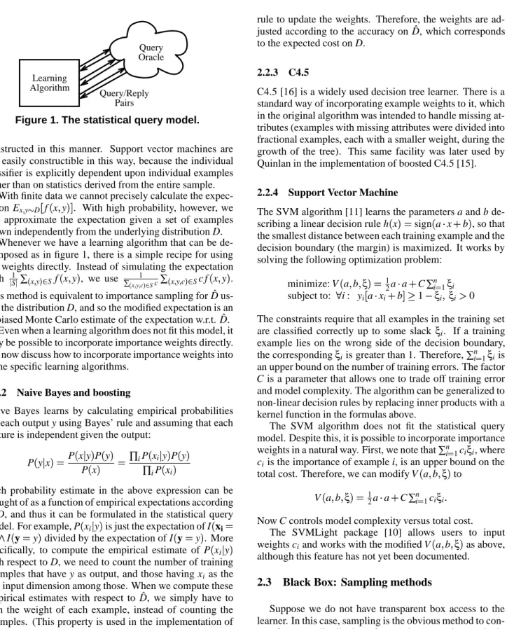
As shown in figure 1, many learning algorithms can be divided into two components: a portion which calculates the (approximate) expected value of some function (or query) f and a portion which forms these queries and uses their output to construct a classifier. For example, neural net-works, decision trees, and Naive Bayes classifiers can be

Learning Algorithm Query/Reply Pairs Query Oracle

Figure 1. The statistical query model.

constructed in this manner. Support vector machines are not easily constructible in this way, because the individual classifier is explicitly dependent upon individual examples rather than on statistics derived from the entire sample.

With finite data we cannot precisely calculate the expec-tation Exy D

f xy. With high probability, however, we can approximate the expectation given a set of examples drawn independently from the underlying distribution D.

Whenever we have a learning algorithm that can be de-composed as in figure 1, there is a simple recipe for using the weights directly. Instead of simulating the expectation with 1 S ∑x y S f xy, we use 1 ∑x yc S c∑x yc S c f xy. This method is equivalent to importance sampling for ˆD us-ing the distribution D, and so the modified expectation is an unbiased Monte Carlo estimate of the expectation w.r.t. ˆD.

Even when a learning algorithm does not fit this model, it may be possible to incorporate importance weights directly. We now discuss how to incorporate importance weights into some specific learning algorithms.

2.2.2 Naive Bayes and boosting

Naive Bayes learns by calculating empirical probabilities for each output y using Bayes’ rule and assuming that each feature is independent given the output:

P yx P xyP y P x ∏i P xiyP y ∏iPxi

Each probability estimate in the above expression can be thought of as a function of empirical expectations according to D, and thus it can be formulated in the statistical query model. For example, P xiy is just the expectation of I xi

xi I y

y divided by the expectation of I y

y. More specifically, to compute the empirical estimate of P xiy with respect to D, we need to count the number of training examples that have y as output, and those having xias the i-th input dimension among those. When we compute these empirical estimates with respect to ˆD, we simply have to sum the weight of each example, instead of counting the examples. (This property is used in the implementation of boosted Naive Bayes [5].)

To incorporate importance weights into AdaBoost [8], we give the importance weights to the weak learner in the first iteration, thus effectively drawing examples from ˆD. In the subsequent iterations, we use the standard AdaBoost

rule to update the weights. Therefore, the weights are ad-justed according to the accuracy on ˆD, which corresponds to the expected cost on D.

2.2.3 C4.5

C4.5 [16] is a widely used decision tree learner. There is a standard way of incorporating example weights to it, which in the original algorithm was intended to handle missing at-tributes (examples with missing atat-tributes were divided into fractional examples, each with a smaller weight, during the growth of the tree). This same facility was later used by Quinlan in the implementation of boosted C4.5 [15].

2.2.4 Support Vector Machine

The SVM algorithm [11] learns the parameters a and b de-scribing a linear decision rule h x

sign ax b , so that the smallest distance between each training example and the decision boundary (the margin) is maximized. It works by solving the following optimization problem:

minimize: V abξ 1 2aa C∑ n i 1ξi subject to: i : yiaxi b 1 ξi ξi 0 The constraints require that all examples in the training set are classified correctly up to some slack ξi. If a training example lies on the wrong side of the decision boundary, the correspondingξiis greater than 1. Therefore,∑ni 1ξi

is an upper bound on the number of training errors. The factor C is a parameter that allows one to trade off training error and model complexity. The algorithm can be generalized to non-linear decision rules by replacing inner products with a kernel function in the formulas above.

The SVM algorithm does not fit the statistical query model. Despite this, it is possible to incorporate importance weights in a natural way. First, we note that∑n_i

1

ciξi, where ciis the importance of example i, is an upper bound on the total cost. Therefore, we can modify V abξ to

V abξ 1 2aa C∑ n i 1 ciξi Now C controls model complexity versus total cost.

The SVMLight package [10] allows users to input weights ciand works with the modified V abξ as above, although this feature has not yet been documented.

2.3

Black Box: Sampling methods

Suppose we do not have transparent box access to the learner. In this case, sampling is the obvious method to con-vert from one distribution of examples to another to obtain a cost-sensitive learner using the translation theorem (The-orem 2.1). As it turns out, straightforward sampling does not work well in this case, motivating us to propose an al-ternative method based on rejection sampling.

2.3.1 Sampling-with-replacement

Sampling-with-replacement is a sampling scheme where each example xyc is drawn according to the distribution p xyc

c

∑x yc Sc

. Many examples are drawn to create a new dataset S . This method, at first pass, appears useful because every example is effectively drawn from the distri-bution ˆD. In fact, very poor performance can result when using this technique, which is essentially due to overfitting because of the fact that the examples in S are not drawn in-dependently from ˆD, as we will elaborate in the section on experimental results (Section 3).

Sampling-without-replacement is also not a solution to this problem. In sampling-without-replacement, an ex-ample xyc is drawn from the distribution pxyc

c ∑x

ycSc

and the next example is drawn from the set S

xyc . This process is repeated, drawing from a smaller and smaller set according to the weights of the examples remaining in the set.

To see how this method fails, note that sampling-without-replacement m times from a set of size m results in the original set, which (by assumption) is drawn from the distribution D, and not ˆD as desired.

2.3.2 Cost-proportionate rejection sampling

There is another sampling scheme called rejection sampling [18] which allows us to draw examples independently from the distribution ˆD, given examples drawn independently from D. In rejection sampling, examples from ˆD are ob-tained by first drawing examples from D, and then keep-ing (or acceptkeep-ing) the sample with probability proportional to ˆD D. Here, we have ˆD D∝c, so we accept an exam-ple with probability c Z, where Z is some constant cho-sen so that max_x

yc S

c Z,

3 _{leading to the name}

cost-proportionate rejection sampling. Rejection sampling re-sults in a set S which is generally smaller than S. Further-more, because inclusion of an example in S is independent of other examples, and the examples in S are drawn inde-pendently, we know that the examples in S are distributed independently according to ˆD.

Using cost-proportionate rejection sampling to create a set S and then using a learning algorithm A S is guaran-teed to produce an approximately cost-minimizing classi-fier, as long as the learning algorithm A achieves approxi-mate minimization of classification error.

Theorem 2.2. (Correctness) For all cost-sensitive sample

sets S, if cost-proportionate rejection sampling produces a sample set S and A S achievesεclassification error:

E_x yc Dˆ I hx y ε 3_{In practice, we choose Z} max x

ywSc so as to maximize the size of

the set S. A data-dependent choice of Z is not formally allowed for

rejec-tion sampling. However, the introduced bias appears small whenS 1.

A precise measurement of “small” is an interesting theoretical problem.

then h

A S approximately minimizes cost:

Exyc D c I hx y εN where N Exyc D c.

Proof. Rejection sampling produces a sample set S drawn independently from ˆD. By assumption A S outputs a clas-sifier h such that

E_x yc Dˆ

I hx

y ε

By the translation theorem (Theorem 2.1), we know that E_x yc Dˆ I hx y 1 NExyc D c I hx y Thus, _E xyc D c I hx y εN

2.3.3 Sample complexity of cost-proportionate rejec-tion sampling

The accuracy of a learned classifier generally improves monotonically with the number of examples in the training set. Since cost-proportionate rejection sampling produces a smaller training set (by a factor of about N Z), one would expect worse performance than using the entire training set. This turns out to not be the case, in the agnostic PAC-learning model [17, 12], which formalizes the notion of probably approximately optimal learning from arbitrary dis-tributions D.

Definition 2.1. A learning algorithm A is said to be an

agnostic PAC-learner for hypothesis class H, with sample complexity m 1 ε1 δ if for all ε

0 and δ 0, m

m 1 ε1 δ is the least sample size such that for all dis-tributions D (over X Y ), the classification error rate of its output h is at mostεmore than the best achievable by any member of H with probability at least 1 δ, whenever the sample size exceeds m.

By analogy, we can formalize the notion of cost-sensitive agnostic PAC-learning.

Definition 2.2. A learning algorithm A is said to be a

cost-sensitive agnostic PAC-learner for hypothesis class H, with cost-sensitive sample complexity m 1 ε1 δ, if for all

ε 0 andδ 0, m

m 1 ε1 δ is the least sample size such that for all distributions D (over X Y C), the ex-pected cost of its output h is at mostε more than the best achievable by any member of H with probability at least 1 δ, whenever the sample size exceeds m.

We will now use this formalization to compare the cost-sensitive PAC-learning sample complexity of two methods: applying a given base classifier learning algorithm to a sam-ple obtained through cost-proportionate rejection sampling, and applying the same algorithm on the original training set. We show that the cost-sensitive sample complexity of the latter method is lower-bounded by that of the former.

Theorem 2.3. (Sample Complexity Comparison) Fix an

arbitrary base classifier learning algorithm A, and sup-pose that morig 1 ε1 δ and mrej 1 ε1 δ, respectively, are cost-sensitive sample complexity of applying A on the original training set, and that of applying A with cost-proportionate rejection sampling. Then, we have

morig 1 ε1 δ

Ω

mrej 1 ε1 δ

Proof. Let m 1 ε1 δ be the (cost-insensitive) sample complexity of the base classifier learning algorithm A. (If no such function exists, then neither morig 1 ε1 δ nor mrej 1 ε1 δ exists, and the theorem holds vacuously.) Since Z is an upper bound on the cost of misclassifying an example, we have that the cost-sensitive sample complexity of using the original training set satisfies

morig 1 ε1 δ

Θ

mZ ε1 δ

This is because given a distribution that forcesεmore clas-sification error than optimal, another distribution can be constructed, that forcesεZ more cost than optimal, by as-signing cost Z to all examples on which A errs.

Now from Theorem 2.2 and noting that the central limit theorem implies that cost-proportionate rejection sampling reduces the sample size by a factor of Θ N Z, the cost-sensitive sample complexity for rejection sampling is:

mrej 1 ε1 δ

Θ

Z

Nm N ε1 δ (1)

A fundamental theorem from PAC-learning theory states that m 1 ε1 δ Ω 1 ε ln1 δ [4]. When m 1 ε1 δ Θ 1 ε ln1 δ, Equation (1) implies: mrej 1 ε1 δ Θ Z N N ε ln1 δ Θ morig 1 ε1 δ Finally, note that when m 1 ε1 δ grows faster than linear in 1 ε, we have mrej 1 ε1 δ

omorig 1 ε1 δ , which finishes the proof.

Note that the linear dependence of sample size on 1 ε is only achievable by an ideal learning algorithm, and in practice super-linear dependence is expected, especially in the presence of noise. Thus, the above theorem implies that cost-proportionate rejection sampling minimizes cost better than no sampling for worst case distributions.

This is a remarkable property about any sampling scheme, since one generally expects that predictive perfor-mance is compromised by using a smaller sample. Cost-proportionate rejection sampling seems to distill the origi-nal sample and obtains a sample of smaller size, which is at least as informative as the original.

2.3.4 Cost-proportionate rejection sampling with ag-gregation (costing)

From the same original training sample, different runs of cost-proportionate rejection sampling will produce differ-ent training samples. Furthermore, the fact that rejection

sampling produces very small samples means that the time required for learning a classifier is generally much smaller.

We can take advantage of these properties to devise an ensemble learning algorithm based on repeatedly perform-ing rejection samplperform-ing from S to produce multiple sample sets S₁ S

m, and then learning a classifier for each set. The output classifier is the average over all learned classi-fiers. We call this technique costing:

Costing(Learner A, Sample Set S, count t)

1. For i

1 to t do (a) S

rejection sample from S with acceptance probability c Z. (b) Let hi A S 2. Output h x sign ∑t_i 1 hi x

The goal in averaging is to improve performance. There is both empirical and theoretical evidence suggesting that averaging can be useful. On the empirical side, many peo-ple have observed good performance from bagging despite throwing away a 1 e fraction of the samples. On the theo-retical side, there has been considerable work which proves that the ability to overfit of an average of classifiers might be smaller than naively expected when a large margin ex-ists. The preponderance of learning algorithms producing averaging classifiers provides significant evidence that av-eraging is useful.

Note that despite the extra computational cost of averag-ing, the overall computational time of costing is generally much smaller than that of a learning algorithm using sam-ple set S (with or without weights). This is the case because most learning algorithms have running times that are super-linear in the number of examples.

3

Empirical evaluation

We show empirical results using two real-world datasets. We selected datasets that are publicly available and for which cost information is available on a per example ba-sis. Both datasets are from the direct marketing domain. Although there are many other data mining domains that are cost-sensitive, such as credit card fraud detection and medical diagnosis, publicly available data are lacking.

3.1

The datasets used

3.1.1 KDD-98 dataset

This is the well-known and challenging dataset from the KDD-98 competition, now available at the UCI KDD repos-itory [9]. The dataset contains information about persons who have made donations in the past to a particular charity. The decision-making task is to choose which donors to mail a request for a new donation. The measure of success is the total profit obtained in the mailing campaign.

The dataset is divided in a fixed way into a training set and a test set. Each set consists of approximately 96000 records for which it is known whether or not the person made a donation and how much the person donated, if a do-nation was made. The overall percentage of donors is about 5%. Mailing a solicitation to an individual costs the charity $068. The donation amount for persons who respond varies from $1 to $200. The profit obtained by soliciting every in-dividual in the test set is $10560, while the profit attained by the winner of the KDD-98 competition was $14712.

The importance of each example is the absolute dif-ference in profit between mailing and not mailing an in-dividual. Mailing results in the donation amount minus the cost of mailing. Not mailing results in zero profit. Thus, for positive examples (respondents), the importance varies from $032 to $19932. For negative examples (non-respondents), it is fixed at $068.

3.1.2 DMEF-2 dataset

This dataset can be obtained from the DMEF dataset library [1] for a nominal fee. It contains customer buying history for 96551 customers of a nationally known catalog. The decision-making task is to choose which customers should receive a new catalog so as to maximize the total profit on the catalog mailing campaign. Information on the cost of mailing a catalog is not available, so we fixed it at $2.

The overall percentage of respondents is about 2.5%. The purchase amount for customers who respond varies from $3 to $6247. As is the case for the KDD-98 dataset, the importance of each example is the absolute difference in profit between mailing and not mailing a customer. There-fore, for positive examples (respondents), the importance varies from $1 to $6245. For negative examples (non-respondents), it is fixed at $2.

We divided the dataset in half to create a training set and a test set. As a baseline for comparison, the profit obtained by mailing a catalog to every individual on the training set is $26474 and on the test set is $27584.

3.2

Experimental results

3.2.1 Transparent box results

Table 1 (top) shows the results for Naive Bayes, boosted Naive Bayes (100 iterations) C4.5 and SVMLight on the KDD-98 and DMEF-2 datasets, with and without the im-portance weights. Without the imim-portance weights, the clas-sifiers label very few of the examples positive, resulting in small (and even negative) profits. With the costs given as weights to the learners, the results improve significantly for all learners, except C4.5. Cost-sensitive boosted Naive Bayes gives results comparable to the best so far with this dataset [19] using more complicated methods.

We optimized the parameters of the SVM by cross-validation on the training set. Without weights, no setting of the parameters prevented the algorithm of labeling all exam-ples as negatives. With weights, the best parameters were

KDD-98:

Method Without Weights With Weights

Naive Bayes 0.24 12367

Boosted NB -1.36 14489

C4.5 0 118

SVMLight 0 13683

DMEF-2:

Method Without Weights With Weights

Naive Bayes 16462 32608

Boosted NB 121 36381

C4.5 0 478

SVMLight 0 36443

Table 1. Test set profits with transparent box.

a polynomial kernel with degree 3 and C

5 10 5for KDD-98 and a linear kernel with C

00005 for DMEF-2. However, even with this parameter setting, the results are not so impressive. This may be a hard problem for margin-based classifiers because the data is very noisy. Note also that running SVMLight on this dataset takes about 3 orders of magnitude longer than AdaBoost with 100 iterations.

The failure of C4.5 to achieve good profits with impor-tance weights is probably related to the fact that the facil-ity for incorporating weights provided in the algorithm is heuristic. So far, it has been used only in situations where the weights are fairly uniform (such as is the case for frac-tional instances due to missing data). These results indicate that it might not be suitable for situations with highly non-uniform costs. The fact that it is non-trivial to incorporate costs directly into existing learning algorithms is the moti-vation for the black box approaches that we present here.

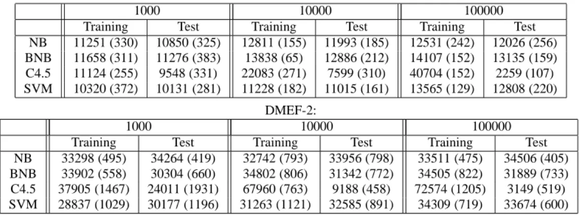
3.2.2 Black box results

Table 2 shows the results of applying the same learn-ing algorithms to the KDD-98 and DMEF-2 data uslearn-ing training sets of different sizes obtained by sampling-with-replacement. For each size, we repeat the experiments 10 times with different sampled sets to get mean and standard error (in parentheses). The training set profits are on the original training set from which we draw the sampled sets.

The results confirm that application of sampling-with-replacement to implement the black box approach can result in very poor performance due to overfitting. When there are large differences in the magnitude of importance weights, it is typical for an example to be picked twice (or more). In table 2, we see that as we increase the sampled training set size and, as a consequence, the number of duplicate exam-ples in the training set, the training profit becomes larger while the test profit becomes smaller for C4.5.

Examples which appear multiple times in the training set of a learning algorithm can defeat complexity control mech-anisms built into learning algorithms For example, suppose that we have a decision tree algorithm which divides the training data into a “growing set” (used to construct a tree)

KDD-98:

1000 10000 100000

Training Test Training Test Training Test NB 11251 (330) 10850 (325) 12811 (155) 11993 (185) 12531 (242) 12026 (256) BNB 11658 (311) 11276 (383) 13838 (65) 12886 (212) 14107 (152) 13135 (159) C4.5 11124 (255) 9548 (331) 22083 (271) 7599 (310) 40704 (152) 2259 (107) SVM 10320 (372) 10131 (281) 11228 (182) 11015 (161) 13565 (129) 12808 (220) DMEF-2: 1000 10000 100000

Training Test Training Test Training Test

NB 33298 (495) 34264 (419) 32742 (793) 33956 (798) 33511 (475) 34506 (405) BNB 33902 (558) 30304 (660) 34802 (806) 31342 (772) 34505 (822) 31889 (733) C4.5 37905 (1467) 24011 (1931) 67960 (763) 9188 (458) 72574 (1205) 3149 (519) SVM 28837 (1029) 30177 (1196) 31263 (1121) 32585 (891) 34309 (719) 33674 (600)

Table 2. Profits using sampling-with-replacement.

and a “pruning set” (used to prune the tree for complex-ity control purposes). If the pruning set contains examples which appear in the growing set, the complexity control mechanism is defeated.

Although not as markedly as for C4.5, we see the same phenomenon for the other learning algorithms. In general, as the size of the resampled size grows, the larger is the dif-ference between training set profit and test set profit. And, even with 100000 examples, we do not obtain the same test set results as giving the weights directly to Boosted Naive Bayes and SVM.

The fundamental difficulty here is that the samples in S are not drawn independently from ˆD. In particular, if ˆD is a density, the probability of observing the same example twice given independent draws is 0, while the probability using sampling-with-replacement is greater than 0. Thus sampling-with-replacement fails because the sampled set S is not constructed independently.

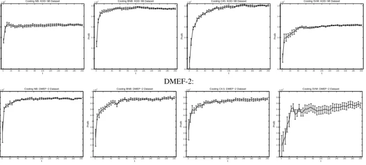
Figure 2 shows the results of costing on the KDD-98 and DMEF-2 datasets, with the base learners and Z

200 or Z

6247, respectively. We repeated the experiment 10 times for each t and calculated the mean and standard error of the profit. The results for t

1, t

100 and t

200 are also given in table 3.

In the KDD-98 case, each resampled set has only about 600 examples, because the importance of the examples varies from 0.68 to 199.32 and there are few “important” examples. About 55% of the examples in each set are pos-itive, even though on the original dataset the percentage of positives is only 5%. With t

200, the C4.5 version yields profits around $15000, which is exceptional performance for this dataset.

In the DMEF-2 case, each set has only about 35 exam-ples, because the importances vary even more widely (from 2 to 6246) and there are even fewer examples with a large importance than in the KDD-98 case. The percentage of positive examples in each set is about 50%, even though on the original dataset it was only 2.5%.

For learning the SVMs, we used the same kernels as we did in section 2.2 and the default setting for C. In that

KDD-98: 1 100 200 NB 11667 (192) 13111 (102) 13163 (68) BNB 11377 (263) 14829 (92) 14714 (62) C4.5 9628 (511) 14935 (102) 15016 (61) SVM 10041 (393) 13075 (41) 13152 (56) DMEF-2: 1 100 200 NB 26287 (3444) 37627 (335) 37629 (139) BNB 24402 (2839) 37376 (393) 37891 (364) C4.5 27089 (3425) 36992 (374) 37500 (307) SVM 21712 (3487) 33584 (1215) 35290 (849)

Table 3. Test set profits using costing.

section, we saw that by feeding the weights directly to the SVM, we obtain a profit of $13683 on the KDD-98 dataset and of $36443 on the DMEF-2 dataset. Here, we obtain profits around $13100 and $35000, respectively. However, this did not require parameter optimization and, even with t

200, was much faster to train. The reason for the speed-up is that the time complexity of SVM learning is generally superlinear in the number of training examples.

4

Discussion

Costing is a technique which produces a cost-sensitive classification from a cost-insensitive classifier using only black box access. This simple method is fast, results in ex-cellent performance and often achieves drastic savings in computational resources, particularly with respect to space requirements. This last property is especially desirable in applications of cost-sensitive learning to domains that in-volve massive amount of data, such as fraud detection, tar-geted marketing, and intrusion detection.

Another desirable property of any reduction is that it ap-plies to the theory as well as to concrete algorithms. Thus, the reduction presented in the present paper allows us to au-tomatically apply any future results in cost-insensitive clas-sification to cost-sensitive clasclas-sification. For example, a

KDD-98: 0 20 40 60 80 100 120 140 160 180 200 0.9 1 1.1 1.2 1.3 1.4 1.5 x 104 t Profit Costing NB: KDD−98 Dataset 0 20 40 60 80 100 120 140 160 180 200 0.9 1 1.1 1.2 1.3 1.4 1.5 x 104 t Profit Costing BNB: KDD−98 Dataset 0 20 40 60 80 100 120 140 160 180 200 0.9 1 1.1 1.2 1.3 1.4 1.5 x 104 t Profit Costing C45: KDD−98 Dataset 0 20 40 60 80 100 120 140 160 180 200 0.9 1 1.1 1.2 1.3 1.4 1.5 x 104 t Profit Costing SVM: KDD−98 Dataset DMEF-2: 0 20 40 60 80 100 120 140 160 180 200 1.8 2 2.2 2.4 2.6 2.8 3 3.2 3.4 3.6 3.8 4x 10 4 t Profit

Costing NB: DMEF−2 Dataset

0 20 40 60 80 100 120 140 160 180 200 1.8 2 2.2 2.4 2.6 2.8 3 3.2 3.4 3.6 3.8 4x 10 4 t Profit

Costing BNB: DMEF−2 Dataset

0 20 40 60 80 100 120 140 160 180 200 1.8 2 2.2 2.4 2.6 2.8 3 3.2 3.4 3.6 3.8 4x 10 4 t Profit

Costing C4.5: DMEF−2 Dataset

0 20 40 60 80 100 120 140 160 180 200 1.8 2 2.2 2.4 2.6 2.8 3 3.2 3.4 3.6 3.8 4x 10 4 t Profit

Costing SVM: DMEF−2 Dataset

Figure 2. Costing: test set profit vs. number of sampled sets.

bound on the future error rate of A S implies a bound on the expected cost with respect to the distribution D. This additional property of a reduction is especially important because cost-sensitive learning theory is still young and rel-atively unexplored.

One direction for future work is multiclass cost-sensitive learning. If there are K classes, the minimal representation of costs is K 1 weights. A reduction to cost-insensitive classification using these weights is an open problem.

References

[1] Anifantis, S. The DMEF Data Set Library. The Di-rect Marketing Association, New York, NY, 2002.

[http://www.the-dma.org/dmef/dmefdset.shtml]

[2] Domingos, P. MetaCost: A general method for making classi-fiers cost sensitive. Proceedings of the 5th International

Con-ference on Knowledge Discovery and Data Mining, 155-164,

1999.

[3] Drummond, C. & Holte, R. Exploiting the cost (in)sensitivity of decision tree splitting criteria. Proceedings of the 17th

In-ternational Conference on Machine Learning, 239-246, 2000.

[4] Ehrenfeucht, A., Haussler, D., Kearns, M. & Valiant. A gen-eral lower bound on the number of examples needed for learn-ing. Information and Computation, 82:3, 247-261, 1989. [5] Elkan, C. Boosting and naive bayesian learning (Technical

Report). University of California, San Diego, 1997.

[6] Elkan, C. The foundations of cost-sensitive learning.

Proceed-ings of the 17th International Joint Conference on Artificial Intelligence, 973-978, 2001.

[7] Fan, W., Stolfo, S., Zhang, J. & Chan, P. AdaCost: Misclas-sification cost-sensitive boosting. Proceedings of the 16th

In-ternational Conference on Machine Learning, 97-105, 1999.

[8] Freund, Y. & Schapire, R. E. A decision-theoretic generaliza-tion of on-line learning and an applicageneraliza-tion to boosting. Journal

of Computer and System Sciences, 55:1, 119-139, 1997.

[9] Hettich, S. & Bay, S. D. The UCI KDD Archive. University of California, Irvine.[http://kdd.ics.uci.edu/]. [10] Joachims, T. Making large-scale SVM learning practical. In

Advances in Kernel Methods - Support Vector Learning. MIT

Press, 1999.

[11] Joachims, T. Estimating the generalization performance of a SVM efficiently. Proceedings of the 17th International

Con-ference on Machine Learning, 431-438, 2000.

[12] Kearns, M., Schapire, R., & Sellie, L. Toward Efficient Ag-nostic Learning. Machine Learning, 17, 115-141, 1998. [13] Kearns, M. Efficient noise-tolerant learning from statistical

queries. Journal of the ACM, 45:6, 983-1006, 1998.

[14] Margineantu, D. Class probability estimation and cost-sensitive classification decisions. Proceedings of the 13th

Eu-ropean Conference on Machine Learning, 270-281, 2002.

[15] Quinlan, J. R. Boosting, Bagging, and C4.5. Proceedings of

the Thirteenth National Conference on Artificial Intelligence,

725-730, 1996.

[16] Quinlan, J. R. C4.5: Programs for Machine Learning. San Mateo, CA: Morgan Kaufmann, 1993.

[17] Valiant, L. A theory of the learnable. Communications of the

ACM, 27:11, 1134-1142, 1984.

[18] von Neumann, J. Various techniques used in connection with random digits, National Bureau of Standards, Applied

Mathe-matics Series, 12, 36-38, 1951.

[19] Zadrozny, B. and Elkan, C. Learning and making decisions when costs and probabilities are both unknown. Proceedings

of the 7th International Conference on Knowledge Discovery and Data Mining, 203-213, 2001.