An Experimental Comparison of Three Guiding Principles for the Detection of
Salient Image Locations: Stability, Complexity, and Discrimination
Dashan Gao
Nuno Vasconcelos
Department of Electrical and Computer Engineering,
University of California, San Diego
[email protected]
[email protected]
Abstract
We present an experimental comparison of the performance of representative saliency detectors from three guiding prin-ciples for the detection of salient image locations: locations of maximum stability with respect to image transformations, locations of greatest image complexity, and most discrimi-nant locations. It is shown that discrimidiscrimi-nant saliency per-forms better in terms of 1) capturing relevant information for classification, 2) being more robust to image clutter, and 3) exhibiting greater stability to image transformations as-sociated with variations of 3D object pose. We then investi-gate the dependence of discriminant saliency on the under-lying set of candidate discriminant features, by comparing the performance achieved with three popular feature sets: the discrete cosine transform, a Gabor, and a Haar wavelet decomposition. It is show that, even though different feature sets produce equivalent results, there may be advantages in considering features explicitly learned from examples of the image classes of interest.
1. Introduction
Saliency mechanisms play an important role in the ability of biological vision systems to perform visual recognition from cluttered scenes. In the computer vision literature, the extraction of salient points from images has been a subject of research for, at least, a few decades. Broadly speaking, existing saliency detectors can be divided into four major classes.
The first, and most popular, treats the problem as one of the detection of specific visual attributes. These are usually edges or corners (also called “interest points”). For exam-ple, Harris [1] and F¨ostner [2] measure an auto-correlation matrix at each image location and then compute its eigen-values to determine whether that location belongs to a flat image region, an edge, or a corner. While these detectors are optimal in the sense of finding salient locations of maximal stability with respect to certain image transformations, there have also been proposals for the detection of other low-level visual attributes, e.g. contours [3]. These basic detectors
can then be embedded in scale-space [12], to achieve de-tection invariance with respect to transformations such as scale [13], or affine mappings [14].
A second major class of saliency detectors is based on more generic, data-driven, definitions of saliency. In par-ticular, an idea that has recently gained some popularity is to define saliency as image complexity. Various complex-ity measures have been proposed: Lowe [4] measures com-plexity by computing the intensity variation in an image us-ing the difference of Gaussian function; Sebe [5] measures the absolute value of the coefficients of a wavelet decompo-sition of the image; and Kadir [6] relies on the entropy of the distribution of local image intensities. The main advan-tage of the definitions in this class is a significantly greater flexibility, that makes them able to detect any of the low-level attributes discussed above (corners, contours, smooth edges, etc.) depending on the image under consideration.
A third formulation is to start from models of
biologi-cal vision, and derive saliency detection algorithms from
these models [7, 22]. This formulation has the appeal of its roots on what are the only known full-functioning vision systems, and has been shown to lead to interesting saliency behavior [7,22]. Interestingly, however, human experiments conducted by the proponents of some of these models have shown that, even in relatively straightforward saliency ex-periments, where subjects are 1) shown images that they have already seen and 2) simply asked to point out salient regions, people do not seem to agree on more than about
50%of the salient locations [22]. This seems to rule out all saliency principles that, like those discussed so far, are ex-clusively based on universal laws which do not depend on some form of 1) context (e.g. a higher level goal that drives saliency) or 2) interpretation of image content.
A final formulation that addresses this problem is di-rectly grounded on the recognition problem, equating
saliency to discriminant power: it defines salient locations
as those that most differentiate the visual class of interest from all others [10,11,15]. Under this formulation, saliency requires a preliminary stage of feature selection, based on some suitable measure of how discriminant each feature is
with respect to the visual classes that compose the recogni-tion problem. In [15], it was shown that this can be done with reduced complexity and, once a set of discriminant fea-tures is available, discriminant saliency can be implemented with very simple, biologically inspired, mechanisms. It was also shown that discriminant saliency leads to higher classi-fication accuracy than that obtained with saliency detectors based on “universal” definitions of salient points.
Various important aspects of discriminant saliency were, however, not fully investigated in [15]. For example, the re-peatability of the salient points resulting from the proposed discriminant saliency detector was never compared to that of the salient points produced by the definitions of saliency which specifically seek optimality with respect to stability to image transformations. Also, given the close connec-tion between saliency and the discriminant power of the se-lected set of features, it appears likely that the choice of the pool of candidate features from which this set is drawn can have a significant impact on the quality of the saliency judgments. The design of this initial feature set was not dis-cussed in [15], where the discrete cosine transform (DCT) was adopted without much consideration for possible alter-native feature spaces. In this work, we address these ques-tions by presenting the results of a detailed experimental evaluation of the performance of various saliency detectors. This experimental evaluation was driven by two main goals: 1) to compare the performance of representative detectors from three of the saliency principles discussed above (sta-bility, complexity, and discrimination), and 2) to investigate how the performance of the discriminant saliency detector proposed in [15] is affected by both the choice of features and the stability of the resulting salient points.
The paper is organized as follows. Section 2 briefly re-views the saliency detectors used in our comparison: the discriminant saliency detector of [15], a multiscale exten-sion of the popular Harris interest point detector [1], and the scale saliency detector of [6]. Section 3 presents a com-parison of the robustness of the salient locations produced by the three saliency detectors. It is shown that, somewhat surprisingly, discriminant saliency detection produces more stable salient points not only in the presence of clutter, but also for uncluttered images of objects subject to varying 3D pose. Section 4 then evaluates the impact of the feature set on the performance of the discriminant saliency detector, by considering the feature spaces resulting from the DCT, a Gabor, and a Haar wavelet decomposition. It is shown that, while the three feature sets perform similarly, there may be advantages in explicitly learning optimal features (in a dis-criminant sense) for the image classes of interest. Finally, some conclusions are presented in Section 5.
2. Saliency detection
We start with a brief review of the steps required to imple-ment each of the saliency detectors considered in this work: the Harris saliency detector [1], the scale saliency detector of [6] and the discriminant saliency detector of [15].
2.1. Harris saliency
The Harris detector has its roots in the structure from mo-tion literature. It is based on the observamo-tion that corners are stable under some classes of image transformations, and measures the degree of cornerness of the local image struc-ture [1]. For this, it relies on the auto-correlation matrix,
M(x, y) = X
(u,v)
wu,v∇I(x+u, x+v)∇TI(x+u, x+v)
(1) where
∇I(x) = (Ix(x), Iy(x))T (2)
is the spatial gradient of the image at locationx= (x, y),
and wu,v is a low-pass filter, typically a Gaussian, that smoothes the image derivatives. The vanilla implementa-tion of the Harris detector consists of the following steps.
1. the auto-correlation matrix is computed for each loca-tionx.
2. the saliency of the location is then determined by
SH(x) = det[M(x)]−αtrace2[M(x)] (3) whereαis set to 0.04 [1].
In our experiments, we rely on the following multiscale ex-tension.
1. image is decomposed into a Gaussian pyramid [16]. 2. a saliency map Si(x) is computed at each pyramid
level, using the Harris detector of size7×7.
3. the saliency maps of different scales are combined into a multi-scale saliency map according to
SH(x) = k X i=1 S2 i(x). (4)
A scale is also selected, at each image location, by searching for the pyramid level whose saliency map has strongest response.
4. Salient locations are determined by non-maximum suppression. The location of largest saliency and its spatial scale are first found, and all the neighbors of the location within a circle of this scale are then sup-pressed (set to zero). The process is iterated until all locations are either selected or suppressed.
The Harris detector has been shown to achieve better perfor-mance than various other similar saliency detectors, when images are subject to 2D rotation, scaling, lighting varia-tion, viewpoint change and camera noise [8].
2.2. Scale saliency
This method defines saliency as spatial unpredictability, and relies on measures of the information content of the distrib-ution of image intensities over spatial scale to detect salient locations [6]. It consists of three steps.
1. the entropy,H(s,x), of the histogram of local
inten-sities over the image neighborhood of circular scales, centered atx, is computed.
2. the local maximum of the entropy over scales,H(x),
is determined and the associated scale considered as a candidate scale,sp, for locationx.
3. a saliency map is computed as a weighted entropy,
SS(x) =H(x)W(sp,x) (5) where W(s,x) =s Z ∂ ∂sp(I, s,x) dI
andp(I, s,x)is the histogram of image intensities.
Finally, a clustering stage is applied to the saliency map in order to locate the salient regions.
2.3. Discriminant saliency
In [15], saliency is defined as the search for the visual at-tributes that best distinguish a visual concept from all other concepts that may be of interest. This leads to the formula-tion of saliency as a feature selecformula-tion problem, where salient features are those that best discriminate between the target image class and all others. The saliency detector is imple-mented with the following steps.
1. images are projected into a K-dimensional feature space, and the marginal distribution of each feature re-sponse under each classPXk|Y(x|i), i ∈ {0,1}, k ∈ {0, . . . , K−1}, is estimated by a histogram (24 bins were used in the experiments described in this paper). The features are then sorted by descending marginal diversity,
md(Xk) =< KL[PX
k|Y(x|i)||PXk(x)]>Y (6) where < f(i) >Y= P
M
i=1PY(i)f(i), and
KL[p||q] = R
p(s) logpq((xx))dx the Kullback-Leibler divergence between p and q.
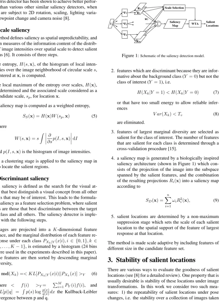
*F1 *Fj *Fn R2 R1 Scale Selection Saliency Map WTA Salient Locations I wi R2n
Figure 1:Schematic of the saliency detection model.
2. features which are discriminant because they are infor-mative about the background class (Y = 0) but not the class of interest (Y = 1), i.e.
H(Xk|Y = 1)< H(Xk|Y = 0) (7) or that have too small energy to allow reliable infer-ences
V ar(Xk)< Tv (8) are eliminated.
3. features of largest marginal diversity are selected as salient for the class of interest. The number of features that are salient for each class is determined through a cross-validation procedure [15].
4. a saliency map is generated by a biologically inspired saliency architecture (shown in Figure 1) which con-sists of the projection of the image into the subspace spanned by the salient features, and the combination of the resulting projectionsRi(x)into a saliency map according to SD(x) = n X i=1 ωiR2i(x), (9)
5. salient locations are determined by a non-maximum suppression stage which sets the scale of each salient location to the spatial support of the feature of largest response at that location.
The method is made scale adaptive by including features of different size in the candidate feature set.
3. Stability of salient locations
There are various ways to evaluate the goodness of salient locations (see [8] for a detailed review). One property that is usually desirable is stability of these locations under image transformations. In this work we consider two such mea-sures: 1) the repeatability of salient locations under pose changes, i.e. the stability over a collection of images taken
under varying viewing conditions, and 2) the robustness of salient locations in the presence of background clutter and intra-class variation, e.g. variable appearance of different objects in the same class. Note that although repeatability under pose change is important for applications such as ob-ject tracking and 3-D reconstruction, the second criterion is more relevant for the recognition from cluttered scenes.
3.1. Stability with respect to clutter and
intra-class variation
For these experiments we relied on the Caltech database, which has been proposed as a testbed for unsupervised ob-ject detection in the presence of clutter [18]. We adopted the experimental set up of [18]: four image classes, faces(435 images), motorbikes(800 images), airplanes (800 images), and rear view of cars (800 images), were used as the classes of interest (Y = 1)1. The Caltech class of “background”
images was used, in all cases, as the “other” class (Y = 0). Although there is a fair amount of intra-class variation in the Caltech database (e.g., the faces of different people ap-pear with different expressions and under variable lighting conditions), there is enough commonality of pose (e.g., all faces are shown in frontal view) to allow the affine mapping of the images into a common coordinate frame, which can be estimated by manually clicking on corresponding points in each image. In this common coordinate frame it is possi-ble to measure the stability of salient locations using a pro-tocol proposed in [9] and which is adopted here. In partic-ular, a salient location is considered a match to a reference image if there exists another salient location in the reference image such that 1) the distance between the two locations is less than half the smallest of the scales associated with them, and 2) the scales of the two locations are within20%
of each other. The average correspondence scoreQis then defined as
Q= T otal number of matches
T otal number of locations. (10)
SupposeNlocations are detected for each of theM images in the database. The scoreQi of reference imageiis the ratio between the total number of matches between that im-age and all otherM−1images in the database, and the total number of salient locations detected in the latter, i.e.,
Qi=
Ni M
N(M −1). (11)
The overall scoreQis the average ofQiover the entire data-base. This score is evaluated as a function of the number of detected regions per image.
1the Caltech image database is available at
http://www.vision.caltech.edu/html-files/archive.html (a) 0 5 10 15 0 5 10 15 20 25 30 35 40 45
Average matching score (%)
Number of top salient locations
S D S H S S (b) 0 5 10 15 20 25 30 0 5 10 15 20 25 30
Number of top salient locations
Average matching score(%)
S D S H S S (c) 0 5 10 15 20 25 30 0 2 4 6 8 10
Number of top salient locations
Average matching score(%)
SD S
H S
S
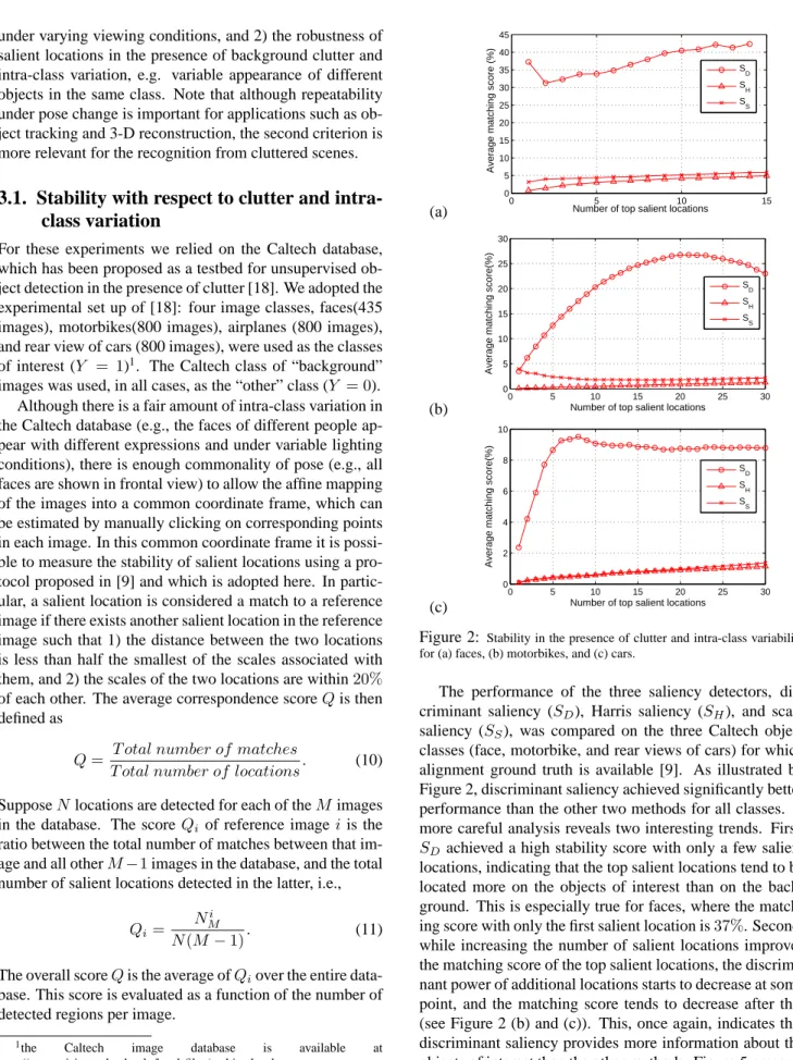
Figure 2: Stability in the presence of clutter and intra-class variability for (a) faces, (b) motorbikes, and (c) cars.
The performance of the three saliency detectors, dis-criminant saliency (SD), Harris saliency (SH), and scale saliency (SS), was compared on the three Caltech object classes (face, motorbike, and rear views of cars) for which alignment ground truth is available [9]. As illustrated by Figure 2, discriminant saliency achieved significantly better performance than the other two methods for all classes. A more careful analysis reveals two interesting trends. First,
SD achieved a high stability score with only a few salient locations, indicating that the top salient locations tend to be located more on the objects of interest than on the back-ground. This is especially true for faces, where the match-ing score with only the first salient location is37%. Second, while increasing the number of salient locations improves the matching score of the top salient locations, the discrimi-nant power of additional locations starts to decrease at some point, and the matching score tends to decrease after that (see Figure 2 (b) and (c)). This, once again, indicates that discriminant saliency provides more information about the objects of interest than the other methods. Figure 5 presents
some examples of salient locations detected by discriminant saliency on Caltech, illustrating how the salient locations are detected robustly, despite substantial changes in appear-ance and significant clutter in the background.
3.2. Stability under 3-D object rotation
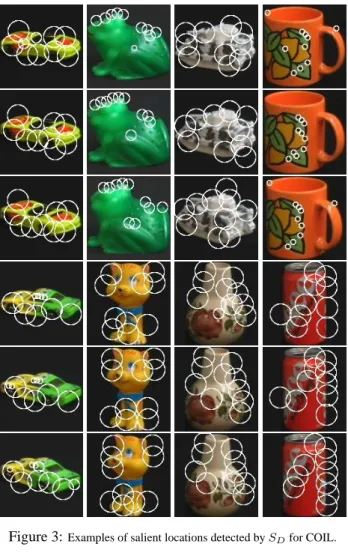
The Columbia Object Image Library (COIL-100) [21] is an appropriate database to evaluate the stability of salient lo-cations under 3-D rotation. It contains images from a set of100 objects,720images from each object, obtained by rotating the object in 3D by5degrees between consecutive views. To avoid the loss of consistence of distinctive fea-tures due to large view-angle change (e.g. the eyes of a sub-ject are not visible from the rear), six consecutive images were used for training and the next three adjacent images (after subsampling so that there are 10 degrees of rotation between views) were used for testing. Sixty objects in the library were used and, for each image, the top ten salient locations were kept. A salient location was considered sta-ble if it appeared in all three test images. The stability was measured by (10).
Table 1 lists the performance of the three saliency de-tectors. Once again, discriminant saliency performed best. This is somewhat surprising, since stability was not directly enforced in the computation of discriminant saliency, and it outperforms Harris, which is designed to be optimal from a stability standpoint. A perfectly reasonable explanation is, however, supported by a closer investigation of the de-tected salient locations. As can be seen from the examples shown in Figure 3, the locations produced by discriminant saliency tend to be locations that maintain a consistent ap-pearance as the object changes pose. This makes intuitive sense since, rather than searching for “salient” points from individual views, discriminant saliency selects features that are “consistently salient” for the whole set of object views in the image class. Or, in other words, under the discrim-inant saliency principle good features are features that ex-hibit small variability of response within the class of interest (while also discriminating between this class and all others). This leads to robust saliency detection if the training set is rich enough to cover the important modes of appearance variability.
4. Influence of features on
discrimi-nant saliency
The good performance of discriminant saliency in the pre-vious set of experiments, motivated us to seek possible
im-SD SH SS
Stability(%) 74.7 71.6 52.2
Table 1:Stability results on the Columbia objects image database.
Figure 3:Examples of salient locations detected bySDfor COIL.
provements to this model. For example, in [15], the au-thors adopted the discrete cosine transform (DCT) feature set without extensive discussion as to why this feature set should be the one of choice. We studied the dependence of discriminant saliency on the underlying features, by com-paring the performance of the DCT to that of two other fea-ture sets.
4.1. Feature sets
A DCT of sizenis the orthogonal transform whose (n×n) basis functions are defined by:
A(i, j) =α(i)α(j) cos(2x+ 1)iπ 2n cos
(2y+ 1)jπ 2n , (12)
where 0 ≤ i, j, x, y < n, α = p1/n for i = 0, and
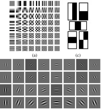
α = p2/n otherwise. According to [15] there are two main reasons to adopt these features. First, they have been shown to perform well on various recognition tasks [17]. Second, as can be seen from Figure 4 (a), many of the DCT basis functions can be interpreted as detectors for various perceptually relevant low-level image attributes, including
(a) (c)
(b)
Figure 4:Basis functions for (a) DCT, (b) Gabor, and (c) Haar features.
edges, corners, t-junctions, and spots. In our experiments, we started by decomposing each image into a four-level Gaussian pyramid. We then computed a multiscale set of DCT features by projecting each pyramid level onto the
8×8DCT basis functions.
The second feature set is based on a Gabor filter bank, which is a set of orientation-specific, band-pass filters. A two dimensional Gabor function can be generally written as
g(x, y) =Kexp(−π(a2(x−x
0)2r+b2(y−y0)2r))
exp(j(2πF0(xcosω0+ysinω0) +P)) (13)
where
(x−x0)r = (x−x0) cosθ+ (y−y0) sinθ
(y−y0)r = −(x−x0) sinθ+ (y−y0) cosθ.
Studies of biological vision have shown that Gabor filters are a good approximation to the sensitivity profiles of neu-rons found in visual cortex of higher vertebrates [19]. For this reason, Gabor filters have been widely used in image analysis for over a decade. The Gabor filter dictionary adopted in these experiments consists of 4 scales and 8 directions (evenly spread from 0 to π), as shown in Fig-ure 4(b). The featFig-ures are also made scale-adaptable by ap-plying to a four-level Gaussian pyramid.
The third feature set is one that has recently become very popular in the computer vision literature, due to its computational efficiency: the Haar decomposition proposed in [20] for real-time object detection. The computational ef-ficiency of this feature set makes it equally attractive for the
saliency problem. As shown in Figure 4(c), five kinds of Haar features were considered in the experiments reported in this work. By varying the size and ratio of the width and height of each rectangle, we generated a set with a total of
330features.
4.2. Classification of saliency maps
To obtain an objective comparison of the different saliency detectors, we adopted the simple classifier-based metric suggested in [15]. This metric consists of feeding an his-togram of saliency map intensities to a classifier and mea-suring the probability of classification error. It quanti-fies how relevant the extracted saliency information is for recognition purposes. Following [15], we relied on a sup-port vector machine (SVM) to classify the saliency his-tograms. The classification experiments were performed on the Caltech database, and performance measured by the receiver-operating characteristic (ROC) equal-error-rate (i.e.p(F alsepositive) = 1−p(T ruepositive)).
The classification results obtained with the different ture sets are presented in Table 2. Although the DCT fea-tures achieved the overall best performance, the other two feature sets were also able to obtain a high classification ac-curacy. For example, discriminant saliency based on any of the three feature sets has performance significantly superior to that achieved by the Harris and scale saliency detectors. While this implies that discriminant saliency is not overly dependent on a unique set of features, these results also sup-port the argument that a feature set with enough variability to represent the distinctive characteristics of the class of in-terest can improve performance. Note, for example, that the Haar features achieve the best performance in the “Air-planes” class. This is not surprising, since a distinctive fea-ture for this class is the elongated airplane body which, in most images, is lighter than the background. While the DCT set lacks a specific detector for this pattern, the bottom left feature of Figure 4 (c) is one such detector, explaining the best performance of the Haar set in this case. An interesting question for future research is, therefore, how to augment the discriminant saliency principle with feature extraction, i.e. the ability to learn the set of features which are most dis-criminant for the class of interest (rather than just selecting a subset from a previously defined feature collection).
Dataset SDDCT SDGabor SDHaar SH SS
Faces 97.24 95.39 93.09 61.87 77.3
Bikes 96.25 96.00 93.50 74.83 81.3
Planes 93.00 93.50 94.75 80.17 78.7
Cars 100.00 98.13 99.88 92.65 90.91 Table 2: SVM classification accuracy based on histograms of saliency maps produced by different detectors.
5. Conclusion
In this work, we have presented an experimental compar-ison of the performance of various saliency detectors. In particular, we have considered detectors representative of three different principles for the detection of salient loca-tions: locations of maximum stability with respect to im-age transformations, locations of greatest imim-age complex-ity, and most discriminant locations. Our results show that discriminant saliency performs better not only from the points of view of 1) capturing more relevant information for classification, and 2) being more robust to image clutter, but also 3) by exhibiting greater stability to image transforma-tions associated with variatransforma-tions of 3D object pose. We have also investigated the dependence of discriminant saliency with respect to the underlying set of candidate discriminant features and found that, even though different feature sets (DCT, Gabor, Haar) worked similarly well, there may be ad-vantages in considering feature sets explicitly learned from examples of the image classes of interest. The design of al-gorithms to optimally learn such features in a discriminant sense remains a topic for future work.
References
[1] C. Harris and M. Stephens. A combined corner and edge de-tector. Alvey Vision Conference, 1988.
[2] F¨orstner. A framework for low level feature ex-traction. Proceedings of European Conference on Computer Vision, p383-394, 1994.
[3] A. Sha’ashua and S. Ullman. Structural saliency: the detec-tion of globally salient structures using a locally connected network. Proc. Internat. Conf. on Computer Vision, 1988. [4] D. G. Lowe. Object recognition from local scale-invariant
features. In Proceedings of International Conference on Computer Vision, pp. 1150-1157, 1999.
[5] N. Sebe, M. S. Lew. Comparing salient point detectors. Pat-tern Recognition Letters, vol.24, no.1-3, Jan. 2003, pp.89-96. [6] T. Kadir and M.l Brady. Scale, Saliency and Image Descrip-tion. International Journal of Computer Vision, Vol.45, No.2, p83-105, November 2001
[7] L. Itti, C. Koch and E. Niebur. A model of saliency-based visual attention for rapid scene analysis. IEEE Trans. Pattern Analysis and Machine Intelligence, 20(11), Nov. 1998. [8] C. Schmid, R. Mohr, and C. Bauckhage. Evaluation of
Inter-est Point Detectors. Int’l J. Computer Vison, 37(2):151-172, 2000
[9] T. Kadir, A. Zisserman, and M. Brady. An affine invari-ant saliency region detector. in Proceedings of ECCV 2004, pp228-241, 2004
[10] B. Schiele and J. Crowley. Where to look next and what to look for. In Intelligent Robots and Systems (IROS’96), pp. 1249-1255, 1996.
[11] K. Walker, T.F. Cootes, and C.J. Taylor. Locating Salient Ob-ject Features. In Proc. of British Machine Vision Conference, pp. 557-566, 1998.
[12] T. Lindeberg. Scale-space theory: A basic tool for analysing structures at different scales. Journal of Applied Statistics,21, 2 (1994), pp. 224C270.
[13] K. Mikolajczyk and C. Schmid. Indexing based on scale in-variant interest points. Proceedings of International Confer-ence on Computer Vision (ICCV01), p525-531, 2001. [14] K. Mikolajczyk and C. Schmid. An affine invariant
inter-est point detector. Proceedings of European Conference on Computer Vision (ECCV02), vol. 1, 128–142, 2002. [15] D. Gao and N. Vasconcelos. Discriminant Saliency for
Vi-sual Recognition from Cluttered Scenes. Proc. Neural Infor-mation Processing System, 2004
[16] P. Burt and E. H. Adelson. The Laplacian Pyramid as a Com-pact Image Code. IEEE Transactions on Communication, COM-31:532-540 (1983).
[17] N. Vasconcelos and G. Carneiro. What is the Role of Inde-pendence for Visual Regognition? In Proc. European Con-ference on Computer Vision, Copenhagen, Denmark, 2002. [18] R. Fergus, P. Perona and A. Zisserman. Object Class
Recog-nition by Unsupervised Scale-Invariant Learning. In Proc. IEEE Conf. on Computer Vision and Pattern Recognition 2003.
[19] J.G. Daugman. Uncertainty relation for resolution in space, spatial frequency, and orientation optimized by two-dimensional visual cortical filters. Journal of the Optical So-ciety of America A, 2(7): 1362-1373, 1985
[20] P. Viola and M. Jones. Robust real-time object detection.2nd
Int. Workshop on Statistical and Computational Theories of Vision Modeling, Learning, Computing and Sampling, July 2001.
[21] S.A. Nene, S.K. Nayar, and H. Murase. Columbia object image library: COIL-100. Technical REport CUCS-006-96, Dept. of Computer Science, Columbia Univ., 1996
[22] C. Privitera, L. Stark. Algorithms for defining visual regions-of-interest: comparison with eye fixations. IEEE Transac-tions on Pattern Analysis & Machine Intelligence, vol.22, no.9, Sept. 2000, pp.970-82.