Modelling skewed spatial random fields through the spatial vine copula

Contents lists available atScienceDirect

Spatial Statistics

journal homepage:www.elsevier.com/locate/spasta

Modelling skewed spatial random fields

through the spatial vine copula

Benedikt Gräler

∗

Institute for Geoinformatics, University of Münster, Heisenbergstr. 2, 48149 Münster, Germany

a r t i c l e i n f o

Article history: Received 28 May 2013 Accepted 7 January 2014 Available online 27 January 2014 Keywords: Spatial copula Multivariate extremes Vine copula Interpolation

a b s t r a c t

Studying phenomena that follow a skewed distribution and entail an extremal behaviour is important in many disciplines. How to describe and model the dependence of skewed spatial random fields is still a challenging question. Especially when one is interested in interpolating a sample from a spatial random field that exhibits extreme events, classical geostatistical tools like kriging relying on the Gaussian assumption fail in reproducing the extremes. Originating from the multivariate extreme value theory partly driven by financial mathematics, copulas emerged in recent years being capable of describing different kinds of joint

tail behaviours beyond the Gaussian realm. In this paperspatial

vine copulas are introduced that are parametrized by distance and allow to include extremal behaviour of a spatial random field. The newly introduced distributions are fitted to the widely studied emergency and routine scenario data set from the spatial interpolation comparison 2004 (SIC2004). The presented spatial vine copula ranks within the top 5 approaches and is superior to all approaches in terms of the mean absolute error.

©2014 The Author. Published by Elsevier B.V.

This is an open access article under the CC BY license (http://creativecommons.org/licenses/by/3.0/).

1. Introduction

Interpolation of spatial random fields is a common task in geostatistics. Simple approaches like inverse distance weighted predictions or the well known kriging procedures have routinely been

∗_{Tel.: +49 251 8333082.}

E-mail address:[email protected]. URL:http://www.ifgi.de/graeler.

http://dx.doi.org/10.1016/j.spasta.2014.01.001

2211-6753/©2014 The Author. Published by Elsevier B.V. This is an open access article under the CC BY license (http:// creativecommons.org/licenses/by/3.0/).

addressing spatial dependence.

The set of methods to model spatial data including extremes is diverse. The different approaches go beyond the field of geostatistics (e.g.Fournier and Furrer, 2005) and incorporate techniques such as neural networks (e.g.Timonin and Savelieva, 2005) or support vector machines (e.g.Pozdnoukhov, 2005) as presented in the spatial interpolation comparison 2004 (SIC2004:Dubois and Galmarini, 2005a). Typically studied spatial phenomena exhibiting extremes are for example radioactive radiation, as in SIC2004, rainfall data (Haberlandt, 2007) or air quality indicators (Horálek et al., 2007). The advantage of thespatial vine copula approach presented in this paper is its flexibility in the selection of appropriate copula families through bivariate spatial copulas.Schepsmeier(2013) suggests an approach where the tree structure of the vine is derived through spatial distances, but the copula families do not change with distance. Another approach modelling several air-quality indicators across a set of stations is briefly introduced byBrechmann(2013) using a hierarchical Kendall copula.

The introduction of a bivariate spatial copula into a vine copula for interpolation has been described byGräler and Pebesma(2011) and is extended in this paper. Convex combinations of bivariate copulas parametrized by distance are combined in avine copula(also known aspair-copula construction:Aas et al.,2009;Bedford and Cooke, 2002) for a local neighbourhood. Adding marginal distributions to the spatial vine copula yields a full multivariate distribution describing a local spatially dependent distribution of the observed phenomenon.

In the following, we will assume a spatial random fieldZ

:

Ω

×

_S

→

_Rdefined over some spatial domain of interestSand probability spaceΩ. Typically, a sampleZ

=



z

(

s1

), . . . ,

z

(

sn

)



has been observed at a set of distinct locationss1

, . . . ,

sn

∈

S. Often, one is interested in modellingZfrom the

sampleZin order to predictZ

(

s0

)

at unobserved locationss0

∈

Sor to simulate the spatial random

field.

The remainder of this paper is organized as follows. The theoretical background of copulas, bivariate spatial copulas and vine copulas yielding the spatial vine copulas, which are the driving probabilistic tool in the applications, are addressed in the following section. A strategy to estimate a spatial vine copula is illustrated in Section3. Section4discusses different uses of the multivariate distribution such as the possibility to predict values at unobserved locations or simulate from the spatial random field. An application is illustrated in Section5where we use the emergency and routine scenario data sets from the SIC2004 (Dubois and Galmarini, 2005a). Results are discussed in Section6. Conclusions are drawn in Section7.

2. Spatial vine copulas

Copulas describe the dependence between the margins of multivariate distributions. Sklar

(1959) proofed that any multivariate distributionH can be split into its margins F1

, . . . ,

Fn and

the copula C which couples the margins with a given dependence structure: H

(

x1

, . . . ,

xn

)

=

C



F1

(

x1

), . . . ,

Fn

(

xn

)



. Many different families exist allowing for very different dependence structures. A copula can be imagined as a multivariate cumulative distribution function on the unit (hyper-) cube with uniform margins where its density reflects the strength of dependence between the margins. For further details we refer to the introductory book byNelsen(2006).

Sklar’s Theorem is true for any dimensiond

≥

2, but we will at first only consider bivariate copulasC

: [

0

,

1

]

2

→ [

0

,

1

]

. The density of a copula (denoted asc) expresses the strength of dependence which changes over the range of the marginal distributions. The only copula exhibiting a

constant strength of dependence across its margins is the product copulaΠdescribing independence. Commonly, strength of dependence in a bivariate setting is measured as a single correlation (or covariance) between two random variables and a Gaussian distribution is often implicitly assumed. As a Gaussian distribution can be decomposed into a Gaussian copula with Gaussian margins, the Gaussian dependence structure is implicitly imposed which is elliptically symmetric (following the notion of elliptical contours of the bivariate Gaussian distribution). Hence, by only investigating the correlation of two variables, one completely neglects the variation in the distribution of the strength of dependence over the range of the variables. Naturally, different copulas might reflect samples of an identical correlation, but their density might show a different pattern. The same applies to the spatial domain where kriging implicitly assumes a Gaussian dependence structure. However, looking into different data sets and investigating pairwise scatter plots reveals non-Gaussian dependence structures. These structures can be captured with copulas.

Incorporating distance as the only parameter but utilizing the flexibility of many bivariate copula families, we introducebivariate spatial copulas. For pairs of locations in a local neighbourhood we assume that the separation distance of these is the driving parameter determining the dependence. Hence, pairs of locations very close to each other are likely to exhibit a dependence structure close to perfect dependence where noise might reduce the strength of dependence to some degree (analogous to the nugget effect in classical kriging). For large distances, the pairs will tend to be independent and are modelled by the product copulaΠ. The approaches byBárdossy(2011) andKazianka and Pilz(2010a) allow only for a single multivariate copula family. The bivariate spatial copulach

(

u

, v)

described here is designed as a convex combination of bivariate copulas (in terms of their densities) that is not limited to a single family (see Eq.(1)). Hence, we allow not only for a varying strength of dependence but also for a changing dependence structure with distance:

ch

(

u

, v)

:=



































c_h(1)

(

u

, v),

0

≤

h

<

l1

(

1

−

λ

₂

)

c_h(1)

(

u

, v)

+

λ

₂c_h(2)

(

u

, v),

l1

≤

h

<

l2

...

...

(

1

−

λ

_k

)

c(_hk−1)

(

u

, v)

+

λ

_k

·

1

,

lk−1

≤

h

<

lk 1

,

lk

≤

h (1) where

λ

j

:=

h−lj−1

lj−lj−1,hdenotes the spatial separating distance of a pair of locations andl1

, . . . ,

lk denote the representative distances of the spatial bins (e.g. midpoint or mean distance of all involved point pairs during the estimation). The parameters of the copulasc_h(i)in the convex combination may as well depend on the distanceh. This allows for a smoothly changing strength of dependence and complete parametrization by distance. The argumentsuand

v

are the values of the modelled pairs of locations transformed to the unit interval

(

0

,

1

)

with the help of the marginal cumulative distribution functions or a rank order transformation. Inspecting Eq.(1)reveals that different choices of bins will in general yield different approximations to the underlying spatial dependence structure. The choice of the binning typically has to balance the two aspects of too little flexibility using few but well filled bins and too few observed pairs per bin using many bins achieving a high flexibility. Its important to ensure a reasonable number of data pairs per bin allowing for a sensible copula estimation.

Concentrating on a local neighbourhood ofdneighbours, we now model the pair-wise dependence between locations through a bivariate spatial copula. However, these copulas need to be joined to benefit from the fulld-dimensional distribution of the neighbourhood. A technique to combine bivariate copulas into multivariate copulas has been introduced byAas et al.(2009) building on work fromBedford and Cooke(2002). This approach has first been introduced as thepair-copula construction

and the resulting copulas are now known asvine copulasin the literature.

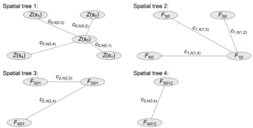
Vine copulas allow to approximate multivariate copulas through bivariate building blocks (see

Fig. 1). The joint density is then obtained as the product of all involved bivariate copula densities. In the general case of spatial vine copulas, where we model the trees up to a certain level 1

≤

l

≤

d

Fig. 1. Graphical representation of a pure spatial vine copula of dimension 5. All trees are spatial trees capturing the depend-ence between the central locations0and its 4 nearest neighbours in ascending orders1, . . . ,s4. The nodes in the vine represent

spatial locations and the length of the connecting edgeh(j−1,k)in each treejrepresents the distance between locationssj−i andskparametrizing the bivariate spatial copulacj−1,h(j−1,k).

and family, we obtain:

ch

(

u0

, . . . ,

ud

)

=

d



i=1 c_0,h(0,i)

(

u0

,

ui

)

·

l−1



j=1 d−j



i=1 cj,h(j,j+i)

(

uj|0,...,j−1

,

uj+i|0,...,j−1

)

·

d−1



j=l d−j



i=1 cj,j+i|0,...,j−1

(

uj|0,...,j−1

,

uj+i|0,...,j−1

)

(2) whereui

=

Fi



Z

(

si

)



for 0

≤

i

≤

d,

uj+i|0,...,j−1

=

Fj−1,h(j−1,j+i)

(

uj+i

|u

0

, . . . ,

uj−1

)

=

∂

Cj−1,h(j−1,j+i)

(

uj−1|0,...,j−2

,

uj+i|0,...,j−2

)

∂

uj−1|0,...,j−2

with 1

≤

j

<

l, 0

≤

i

≤

d

−

jand for the non-spatially varying upper part of the vine

uj+i|0,...,j−1

=

Fj+i|0,...,j−1

(

uj+i

|u

0

, . . . ,

uj−1

)

=

∂

Cj−1,j+i|0,...,j−2

(

uj−1|0,...,j−2

,

uj+i|0,...,j−2

)

∂

uj−1|0,...,j−2

withl

≤

j

<

dand 0

≤

i

≤

d

−

j.

In general, different decompositions of a multivariate copula exist, referred to as regular vines, but in the spatial interpolation where a central element is naturally identified, we use a canonical vine where all initial dependencies are with respect to the central location. In each spatial tree 0

≤

j

<

lof the spatial vine (seeFig. 1), all edges are modelled through a spatial copulacj,h(j,k)parametrized by the

spatial distance between the (conditioned) data pairs of the conditioning locationsjand a member of

the neighbourhoodsk. Once a level is approached where the influence of the spatial distance vanishes,

the consecutive upper trees might be modelled through spatially constant copulas. This spatially fixed upper vine structure does not impose any restriction on the bivariate copulas involved and are kept fixed no matter how the neighbourhood might be spatially organized. The conditional distribution functions involved in the above equations can immediately be obtained as partial derivatives of the already modelled copulasCj−1,j+i|0,...,j−2.

To achieve a full distribution describing the local behaviour of the spatial random fieldZ, margins need to be fitted and joined with the spatial vine copula. Depending on the properties of the

phenomenon to be modelled, one might use a single margin for all locations (in case the random field can be assumed to be stationary) or several margins incorporating some trend that is based for example on location, elevation or additional covariates. The density of the full distribution is obtained by multiplying the copula’s density with the marginal densities and the variables are mapped to the copula scale through the cumulative distribution functions of the marginsF0

, . . . ,

Fd:

fh

(

z0

, . . . ,

zd

)

=

d



i=0 f_i

(

z_i

)

·

ch



F₀

(

z₀

), . . . ,

F_d

(

z_d

)



(3) where theziare representations of the random fieldZ

(

si

)

. Even though copulas allow to separately

model the dependence structure and the margins of a distribution, a successful application requires good fits of both components.

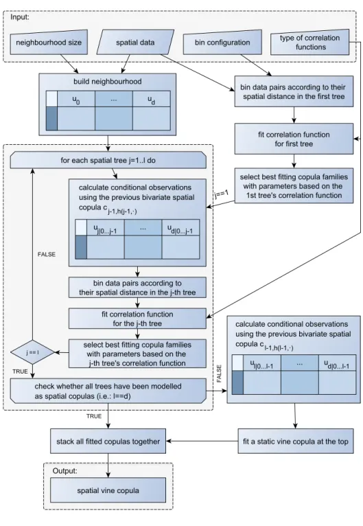
3. Spatial vine copula estimation

In the following, we introduce an estimation procedure for the spatial vine copula that borrows ideas from classical geostatistical approaches. A flow chart illustrating the estimation procedure of a spatial vine copula is shown inFig. 2. To estimate the first bivariate spatial copula, all spatial data is grouped into bins pairwise according to their spatial separation distance. Kendall’s tau correlation measure is marginal independent and thus represents the correlation at the copula level. This makes it very useful in the application of copulas and some one-parameter copula families exhibit a one-to-one relationship between Kendall’s tau and their parameter. The correlogram, using Kendall’s tau, is calcu-lated for the binned data. For each bin several copula families are fitted to the rank-order transformed data and the best fitting family (based on e.g. likelihood, AIC or BIC) is selected. When one restricts the set of copula families to those exhibiting a direct link between Kendall’s tau and their parameter, one might fit a function to the afore obtained empirical correlogram. Thus, the separating distance is used two-fold providing through Kendall’s tau a parameter estimate for the copulas involved in the convex combination and tuning the weight

λ

. This way, the bivariate spatial copula will exactly reproduce Kendall’s tau for any distance as modelled through the function from the correlogram. In case several best fitting families cannot be parametrized through Kendall’s tau, one representative fit for each bin is obtained with a fixed parameter and combined as given in Eq.(1). Using these static representatives in the convex combination of copulas produces Kendall’s tau values as a piecewise linear interpola-tion of the empirical values obtained in the correlogram. The reproducinterpola-tion of Kendall’s tau through the bivariate spatial copulachcan be seen from the fact that a copula’s Kendall’s tau value relies on

the double integral of the copula (Nelsen, 2006, Theorem 5.1.3). For any distanceh, this integration of a convex combination results in a convex combination of two Kendall’s tau values. This pair is either identical, in case the one-to-one relationship between Kendall’s tau and the parameter is utilized or equals the corresponding bins’ values resulting in the piecewise linear interpolation.

For further processing, the data needs to be grouped in neighbourhoods of central locations and their closestd

ˆ

neighbours. The size of these neighbourhoods depends on the dimensiondof the spatial vine copula sought and the number of spatial trees. Iteratively, data pairs are selected from the neighbourhoods based on their spatial distance in the corresponding tree and re-arranged in spatial bins. In the case ofd

= ˆ

dthis reduces the pairs of locations for the last tree to the length of the sample that might be too short for a flexible binning. To increase the number of data pairs in the estimation of the consecutive spatial trees, it is beneficial to use a neighbourhood extending beyond the dimension of the spatial vine copula (d

≤ ˆ

d) thus adding additional location pairs to each binning step for all trees. A rank-order transformation of these neighbourhoods generates ad

ˆ

+

1-dimensional data set with uniform margins distributed on

(

0

,

1

)

.

The bivariate spatial copulac_0,h(0,·)on the first tree can now be used to derive the conditional

sample of dimensiond

ˆ

(conditioned to the value at the central locations0) to which the remainder

of the spatial vine is fitted (seeFigs. 1and2). This conditional sample is again grouped into bins according to the spatial distance of the involved pairs

(

s1

,

s2

)

,

(

s1

,

s3

), . . . , (

s1

,

sd

)

and a second spatial

Fig. 2. Flow chart of the estimation of a spatial vine copula.

closest neighbourss1reduces its dimension again by 1. The procedure of rearranging the data into

bins, estimating the next tree’s spatial copula and conditioning the neighbourhood once more can be repeated until the desired level of spatial copulas is reached. Given that the vine needs to be completed, the (repeatedly) spatially conditioned neighbourhood is used as initial data set for the

spatially fixed upper canonical vine. The vine copula estimation proceeds sequentially by using the best fitting copula per bivariate pair (details are provided inAas et al.(2009),Czado et al.(2012) andDissmann et al.(2013)).

The joint copula densitychcan then be obtained through Eq.(2)where the first product reflects the first spatial tree. The remaining spatial trees are represented in the second product and the spatially constant trees appear in the third product. Fitting the marginal distributions, following generally any approach available in the literature, yields a full distribution through Eq.(3)describing the local behaviour of the random fieldZ.

4. Prediction and simulation of the spatial random field

The local representation of the random fieldZcan be used for different purposes. A typical task is prediction of the modelled phenomenon at unobserved locations. To produce such predictions from a local neighbourhood, every unobserved location needs to be grouped with its d nearest observed neighbours. Conditioning thed

+

1-dimensional copulachon the observed values, yields a 1-dimensional distribution of the phenomenon. This conditional distribution can then be used to calculate the expected value (see Eq.(4)), median or any other desired quantile (see Eq.(5)) denoting for instance confidence intervals. The predictors are given as:



Zm

(

s0

)

=



R z

·

fh

(

z|z1

, . . . ,

zd

)

dz

=



[0,1] F₀−1

(

u

)

ch



u|u1

, . . . ,

ud



du (4)



Zp

(

s0

)

=

F0−1



C_h−1

(

p|u1

, . . . ,

ud

)



(5) whereui

=

Fi

(

zi

)

=

Fi



Z

(

si

)



for 1

≤

i

≤

das before andp

∈

(

0

,

1

)

the desired fraction (e.gp

=

0

.

5 to obtain the median). The equality for



Zmis based on a probability integral transform. An advantage

of this approach is that the conditional distribution describing the random field at the unobserved location may take any form. This is different from kriging, where every predictive distribution is again a normal distribution. This richer flexibility is supposed to provide better uncertainty estimates. Another advantage that is immediate from Eqs.(4) and (5) is that the only information on the marginals needed is their quantile function. This allows for instance to use approximations derived from the empirical cumulative distribution function without the knowledge of any explicitly known form of the family’s density. However, the empirical cumulative distribution function is typically limited to the domain defined by the smallest and largest observation.

For simulation purposes based on a local distribution only, we suggest a sequential simulation algorithm proceeding along a random path (Journel and Huijbregts, 1978;Gómez-Hernández and Journel, 1993). At first,d

+

1 locations of the target geometry are selected. For these initial locations a complete sample is drawn from the spatial vine copula. In the following, further locations are randomly selected one by one and the univariate conditional copula densitych



u|u1

, . . . ,

ud



based on thednearest neighbours is obtained following the notation of Eq.(4). The estimate is then drawn from this conditional distribution. Inserting this spatial sample on copula scale into the marginal quantile functions yields a simulation on the original scale. Repeated iterations of this procedure produce several realizations of the modelled spatial random fieldZ. Conditional simulations can be obtained by introducing the observed values as additional samples that might be included in the conditioning neighbourhoods. This can be seen as starting the simulation at a point where a couple of simulations have already be drawn. A modeller’s choice is to decide to which degree conditioning variables are preferred over spatially closer already simulated values.

5. Application

As the advantage of this new approach is presumed to lie in the modelling of skewed spatial random fields exhibiting extremes that do not follow a Gaussian dependence structure, we will apply it to the

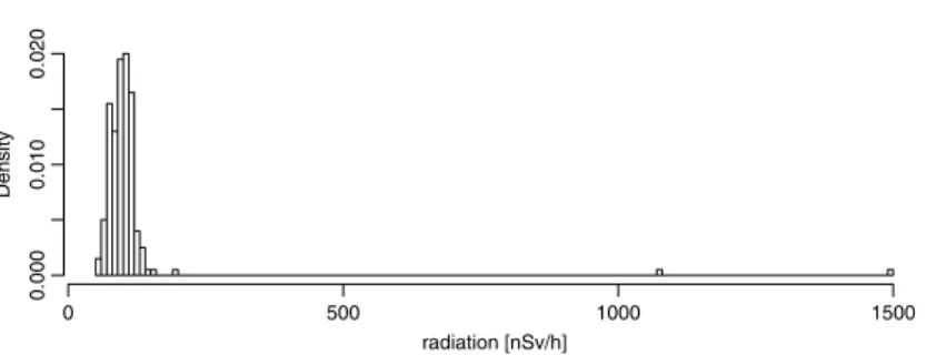
Fig. 3. Histogram of the emergency scenario training data set showing relative frequency. Note that the two columns above 1000 nSv/h only represent a single value each.

emergency scenario data set from the Spatial Interpolation Comparison in 2004 (SIC2004:Dubois and Galmarini, 2005a). This simulated data set was generated from a dispersion process mimicking an accidental release of radioactivity. Following the idea of the spatial interpolation comparison, we apply the spatial vine interpolation procedures as well to the routine data set that only reports low background values. Additionally, we will draw simulations from the modelled spatial random field using the spatial vine copula. All calculations were made using R 3.0.2 (R Core Team, 2013) and can be reproduced by using the publicly available spcopula1_R-package.

Interpolation of the emergency scenario data set

The data consists of 1008 simulated values of which 200 are provided for model fitting and 808 are held back for prediction validation. The area roughly extends to 350 km in east–west and to 700 km in north–south direction.Fig. 3shows a histogram of the emergency scenario training data set. The routine data reports only small background radiations up to 153 nSv/h that as well compose the majority of the emergency scenario. A more detailed description of the data set can be found inDubois and Galmarini(2005a). The data set is freely available and can for instance be obtained through the R-package gstat (Pebesma, 2004).

In a preliminary step, a simple inverse distance weighted interpolation suggests to fit a trend surface to the background data. A linear regression using only the non-extreme data points on the (squared) coordinates x,yand y2 _{provides a reasonable model with an adjusted R}2 _{of 0.41 and}

coefficients being significant at a level of 0.9. The data set consisting of this model’s residuals will be used subsequently.

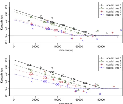
In the following, we follow the repeated binning, spatial copula estimation and conditioning routine as described in Section3and illustrated inFig. 2. The set of families investigated includes the elliptical Gaussian and Student copulas, the Archimedean Clayton, Frank, Gumbel (Nelsen, 2006) and Joe (Joe, 1997) copulas and the survival versions of the latter ones as well as a copula exhibiting cubic and quadratic sections (CQS copula) representing only weaker dependencies (Nelsen, 2006, Example 3.16). All these copula families exhibit a positive dependence and can be parametrized by Kendall’s tau. In case of the two-parameter CQS copula family, the second parameter appears to be constant over space and is fixed at its mean value.Fig. 4shows the graphical representation of the 4 bivariate spatial copulas for the emergency scenario and the routine scenario data sets. The estimation ofc0,h(0,·₎

starts with the entire data set being grouped into spatial bins with bounds at 0 , 20, 30, . . . , 100 km maintaining at least 100 pairs of locations per bin. The estimation of the consecutive bivariate spatial copulasc_1,h(1,·),c2,h(2,·)andc3,h(3,·)to be used in the 2nd, 3rd and 4th spatial tree are initially based on

the 9-dimensional neighbourhoods around the central locations. Thus, each step relies on 200 tuples of (conditional) data being repeatedly rearranged into bins with equally spaced boundaries and filled with roughly 170 pairs of locations each. For each tree, a copula of every family is fitted for each bin with the help of the one-to-one relationship to Kendall’s tau and its log-likelihood is evaluated. The

Fig. 4. Bivariate spatial copulas used in the spatial vine copulas for the emergency scenario (upper panel) and the routine scenario (lower panel). Lines describe the modelled correlation function while symbols represent the empirical values from the binning. Letters denote the chosen copula family: Gaussian (N), student(t), Clayton (C), Frank (F), Gumbel (G), Joe (J), survival Clayton (sC), survival Gumbel (sG) survival Joe (sJ) and one copula based on cubic–quadratic sections (CQ). The product copula (I) representing independence is used for any distance larger than its first appearance.

family with the highest log-likelihood per bin is selected and associated with the mean distance of all pairs of locations of that bin. The set of families and distances determines a bivariate spatial copula per tree. Extending the neighbourhood to 1

+

9 locations increases the number of conditional pairs that can be used to estimate the bivariate spatial copulas at higher trees. Thus a 5-dimensional pure spatial vine copula can be estimated. Additionally, static vine copulas are fitted to the conditioned 5-dimensional neighbourhood using only the first spatial tree and to the 10-dimensional neighbourhood using all 4 spatial trees. Thus, we fit three different spatial vine copulas addressing the models behaviour in terms of neighbourhood size and spatial truncation levell. To illustrate the difference to the Gaussian dependence structure, a spatial Gaussian copula is fitted based on the correlation function of the first tree. Using only the first tree’s correlation function is possible as the spatial Gaussian vine is already completely defined through the spatial correlation matrix given by this unconditioned correlation function (Cooke et al., 2011).

A few model assumptions are made during the estimation process of the different bivariate spatial copulas. The functions relating spatial distance with the value of Kendall’s tau were assumed to be linear and constantly 0 once they hit thex-axis. However, any other function describing this relationship is in general possible. As a consequence, all values of Kendall’s tau are non-negative and only copula families being capable of representing non-negative correlations and having a one-to-one relationship between Kendall’s tau and their parameter have been considered. The copula being defined through its cubic–quadratic sections is in general a two parameter family. However, the second parameter remained mainly constant over the spatial domain and was fixed at the mean value for each bivariate spatial copula. This leads to the desired relationship between Kendall’s tau and the first parameter for this copula as well.

For the comparison study, we compose the above described different spatial vine copulas each for the routine and the emergency scenario. In summary, two are designed for a neighbourhood of 1

+

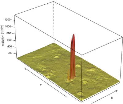
4 locations where one uses only 1 spatial tree and the other is composed completely out of spatial trees

Fig. 5. Surface plot of the median predictor of the pure spatial vine copula with empirical marginal distribution function on a grid spanning the study area.

(denoted ‘‘pure’’). For a neighbourhood of 1

+

9 locations, we investigate the performance for a spatial vine copula using 4 spatial trees (the same as for ‘‘pure’’) followed by a 6-dimensional spatially fixed canonical vine copula at the top. All approaches use the same two types of marginal quantile functions. One type of margin is purely empirical and defined as piecewise linear approximation of the inverse of the empirical cumulative distribution function extended for the ranges of the 99.5%-percentile and 0.5%-percentile to the top and bottom respectively. The second type consists of parametric distributions where in the routine scenario a Gaussian distribution and in the emergency scenario a convex combination of three uniform distributions and a generalized extreme value distribution is used (denoted ‘‘PoT’’). An interpolation of a grid spanning the study area using the median predictor of the pure spatial vine copula and the empirical marginal distribution function is shown inFig. 5.

For each of the spatial vine copulas and the spatial Gaussian copula, we perform the prediction at the 808 locations by predicting the median following Eq.(5). For comparison against classical geostatistical approaches, we perform residual kriging after the trend surface has been subtracted and trans-Gaussian kriging on the original data using the log-transform. The calculations are done using gstat (Pebesma, 2004) while the variograms are fitted using routines provided by the automap package (Hiemstra et al., 2009). To evaluate the performance of the procedures, the mean-absolute error (MAE), root-mean-squared error (RMSE), mean error (ME) and correlation (COR) are calculated between the predicted values and the provided simulated concentrations. All results for the emergency scenario and the routine scenario are summarized inTable 1.

Simulation of the emergency scenario data set

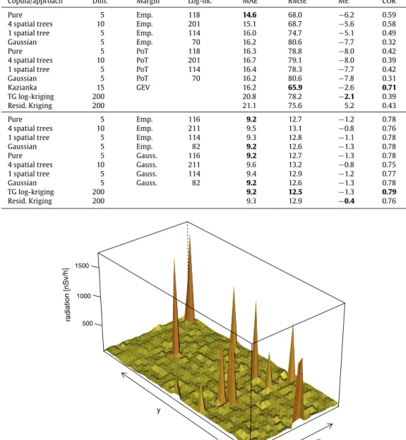
As described in Section4, we simulate from the spatial vine copula using a sequential simulation along a random path. As the small neighbourhood of only four neighbouring locations might lead to unwanted results when clusters emerge from the random path, we adopted a multiple grid strategy (Gómez-Hernández, 1991). The target resolution of the grid is approached step-wise starting with a coarse representation and adding finer grids once all grid points have been simulated. One realization conditioned on the 200 emergency scenario measurements is drawn from the 5-dimensional pure spatial vine and shown inFig. 6.

Table 1

Results for the emergency (upper half) and routine (lower half) scenario. The values of the approach denoted ‘‘Kazianka’’ are taken fromKazianka and Pilz(2010b) where the same data set has been studied. Note that a comparison of log-likelihoods is only possible for the same neighbourhood size. The best performance is indicated in bold.

Copula/approach Dim. Margin Log-lik. MAE RMSE ME COR

Pure 5 Emp. 118 14.6 68.0 −6.2 0.59

4 spatial trees 10 Emp. 201 15.1 68.7 −5.6 0.58

1 spatial tree 5 Emp. 114 16.0 74.7 −5.1 0.49

Gaussian 5 Emp. 70 16.2 80.6 −7.7 0.32

Pure 5 PoT 118 16.3 78.8 −8.0 0.42

4 spatial trees 10 PoT 201 16.7 79.1 −8.0 0.39

1 spatial tree 5 PoT 114 16.4 78.3 −7.7 0.42

Gaussian 5 PoT 70 16.2 80.6 −7.8 0.31

Kazianka 15 GEV 16.2 65.9 −2.6 0.71

TG log-kriging 200 20.8 78.2 −2.1 0.39

Resid. Kriging 200 21.1 75.6 5.2 0.43

Pure 5 Emp. 116 9.2 12.7 −1.2 0.78

4 spatial trees 10 Emp. 211 9.5 13.1 −0.8 0.76

1 spatial tree 5 Emp. 114 9.3 12.8 −1.1 0.78

Gaussian 5 Emp. 82 9.2 12.6 −1.3 0.78

Pure 5 Gauss. 116 9.2 12.7 −1.3 0.78

4 spatial trees 10 Gauss. 211 9.6 13.2 −0.8 0.75

1 spatial tree 5 Gauss. 114 9.4 12.9 −1.2 0.77

Gaussian 5 Gauss. 82 9.2 12.6 −1.3 0.78

TG log-kriging 200 9.2 12.5 −1.3 0.79

Resid. Kriging 200 9.3 12.9 −0.4 0.76

Fig. 6. Surface plot of a conditional simulation of the pure spatial vine copula on a coarse grid spanning the study area.

6. Results and discussion

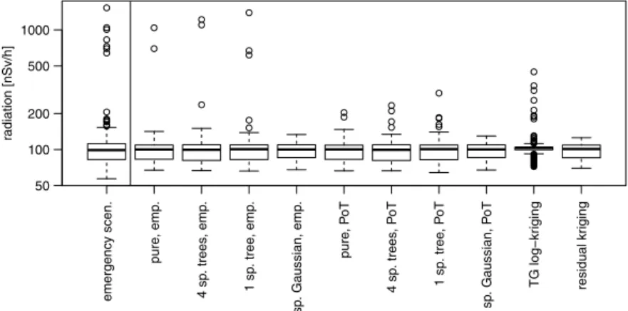
Besides the cross validation results presented inTable 1, it is interesting to observe how well the overall distribution is represented. This is illustrated on log-scale inFig. 7where a box-plot for each method is shown along with the provided 808 data points for validation in the emergency scenario. It is immediate that the trans-Gaussian kriging procedure fails to reproduce the target distribution

Fig. 7. Box-plots (on log-scale) illustrating the overall distribution of the predicted values for the different interpolation approaches along with the provided data set in the emergency application. They-axis is shown in log-scale. The approaches are ordered as inTable 1.

while residual kriging performs a bit better. Just as kriging, the spatial Gaussian copula does not produce any extreme estimates and merely represents the background radiations. The spatial vine copula approaches using the empirical marginal distribution function produce too few extreme values, but within the correct range of the extremes. The predictions based on the theoretical marginal distribution re-produce a moderate heavy right tail, but fail to capture the large extremes. Counting the number of values below the predicted median yields a fraction of about 0.5 for all different copulas supporting this approach. In the routine data case, the box-plots (not shown) are less heterogeneous and all approaches capture the overall marginal distribution rather well.

The same split as in the box-plots (Fig. 7) between the marginal distributions is apparent from

Table 1. Within each group of margins, the spatial Gaussian copula performs slightly worse than the spatial vine copulas. Using the empirical margin that better represents the overall distribution, this difference is pronounced. Hence, the Gaussian copula family fails in capturing the dependence structure of this heavily skewed spatial random field. It does not give fractions large enough to produce extreme quantiles even though the marginal distribution would allow for it. However, the spatial vine copulas only slightly improve the prediction if the marginal distribution function is not capable of reproducing the sample. This stresses the importance of both, a good match in dependence structure and in the marginal distribution function. According to the MAE inTable 1, using more spatial trees improves the prediction. Further improvement of the predictions might be possible for different choices of marginal distributions. An obvious limitation of the empirical distribution function is that the largest value of the 200 records of training data is smaller than the maximum of the 808 target values. Hence, the true extreme values will never be captured using this limited margin. Deeper insights in the process might lead to better marginal distribution functions. However, it will remain challenging to estimate a heavily skewed marginal distribution with only 2 extreme values out of 200 observations.

The best approach reported inDubois and Galmarini(2005b,Table 4) byTimonin and Savelieva

(2005) is based on techniques including neural networks and achieves in the emergency scenario an MAE of 14.9 that is slightly worse than the best spatial vine copula prediction. However, our approaches could not meet the other indicators. Except for the ME, our best performing approach ranks at least within the top 5 of the listed SIC2004 participants and the copula interpolation approach described byKazianka and Pilz(2010b). Taking as well the performance in the routine scenario into account, the median predictor using the pure spatial vine copula with empirical marginal distribution function slightly outperforms the approach byTimonin and Savelieva(2005). However, all approaches are rather close to each other in the routine scenario and hardly distinguishable from their performance indicators.

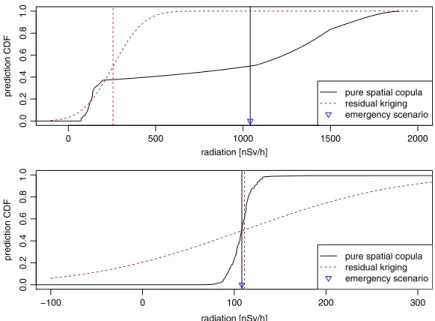
Fig. 8. The predictive cumulative distribution functions for the median predictor of the pure spatial vine copula with empirical marginal distribution function and the residual kriging predictor at an extreme location (upper panel) and at a random background station (lower panel).

Another important aspect is the ability of this approach to flexibly represent the uncertainty in form of a conditional distribution. Different than for the kriging predictor, the conditional distribution may take any form of probability distribution and not only the Gaussian one. InFig. 8the cumulative distribution functions (cdf) of the conditional distributions based on the median predictor of the pure spatial vine copula with empirical marginal distribution function and the residual kriging predictor are compared for two stations in the emergency scenario. It is immediate that the confidence bands in both scenarios differ strongly. The ranges of a confidence band may be both, larger or smaller, for the spatial vine copula than for the kriging approach across the data set. Due to the flexibility to choose any marginal distribution, the copula based approach allows to ensure that its confidence bands do not include any unreasonable values (e.g. negative radiation or concentration) opposed to classical kriging confidence bands that are always symmetric around the predicted mean. This can as well be seen from

Fig. 8where both conditional distributions based on the kriging predictor show (some) probability for negative values. The kriging variance is known to be only dependent on the spatial configuration of the locations. This is different from the spatial vine copula approach where the separating distance and the magnitude of the values influence the conditional predictive distribution. Both uncertainty estimates illustrate how uncertain the model is about its prediction, but neglect uncertainties associated to the model selection and parameter estimation.

In the neighbourhood building step for fitting and prediction, the neighbours are selected by distance only. Given a prominent influence acting on the spatial random field introducing anisotropic dependencies between locations, a more complex neighbourhood selection is likely to be advantageous. Hence, one might want to arrange the neighbourhoods for a 5-dimensional spatial vine copula in such a way that the closest neighbours are selected per (rotated or sheared) quadrant centred ats0 and let theith neighbour always be selected from theith quadrant. For higher dimensional

spatial vine copulas one might split the plane into multiple sectors or select multiple neighbours per quadrant/sector.

The spatial vine copula used in this paper and illustrated in Fig. 1 is only based on spatial dependencies of a single variable. However, additional covariates might be introduced through additional edges in the first tree. These additional edges would then be separately modelled by the best fitting bivariate copula. The sequential structure of the vine would then grow including additional

modelled through the upper trees and their correlation functions. No closed form exists that describes the relationship between the correlations in the upper vine trees and the correlation matrix of the neighbourhood except for the elliptical copula families (Cooke et al., 2011). This leads to the effect that in the local approximation of the spatial random field a pair that does not model any edge of the first spatial trees in two different neighbourhoods might receive different correlation values. This represents the design of a canonical vine with the focus on a single vertex and the contributions of the surrounding vertices to it. The effect of this property on the spatial random field needs to be further investigated.

Methods based on copulas typically increase the computational cost compared to standard approaches such as kriging. Modelling the spatial random field only locally reduces the computational burden and produces predictions outperforming the classical approaches using all available data for the investigated data set. In the presented application, the estimation of the copulas based on 200 locations as well as the prediction at the 808 unobserved locations is done in a few minutes on a common laptop.

The one realization from the spatial vine copula shown inFig. 6shows many more extremes than the one used to condition the simulation. Repeated simulations show that the additional extremes jump over the study area while the true extreme in the lower left quadrant is frequently reproduced. The rather weak spatial dependence and comparatively small spatial neighbourhood leads for some locations to an almost independent sampling from the marginal distribution. This explains the additional extremes scattered across the study area.

7. Conclusion

The presented spatial vine copula approach extends that ofGräler and Pebesma(2011) by using more than one spatial tree at the foundation of the vine. The additional spatial trees add valuable information on the dependence of the higher order neighbours leading to an improved model of the skewed spatial random field. However, further research is needed to develop strategies to select copula families and to fit functions modelling Kendall’s tau in terms of separating distance. Additional model constraints need to be explored to improve the model describing the spatial random field. Negative correlations found in bins were considered to be due to noise in the data in this study. Nevertheless, it needs to be investigated in which scenarios negative correlations may improve the model and how they relate to non-elliptical copulas producing inconsistent spatial correlations for only implicitly modelled pairs of locations.

The introduced spatial vine copula achieves good results in the prediction validation in comparison to the other methods applied to the emergency and routine scenario data sets (Table 1). Hence, the spatial vine copula only predicts extremes where the data is heavily skewed and reproduces the marginal distribution very well compared to residual kriging (Fig. 7). A simpler copula based approach relying on a spatial Gaussian copula is shown to fail in capturing the dependencies of this heavily skewed spatial random field that are successfully modelled by the spatial vine copula. The illustrated flexibility of the conditional marginal distributions describing the uncertainty adds to the value of this new approach.

A spatio-temporal extension of the spatial vine copula with a single spatio-temporal tree has been presented inGräler and Pebesma(2012). The extensions made to the spatial case in this paper are assumed to be applicable to the temporal setting, to improve the interpolation of spatio-temporal data. The directional property of the spatio-temporal domain is likely to introduce asymmetric

dependencies, which can easily be modelled by asymmetric copulas in the bivariate spatio-temporal copulas. This is an advantageous feature of the copula approach in modelling spatio-temporal data.

Acknowledgements

The helpful feedback provided by two anonymous reviewers has been thankfully included. This research has been funded by the German Research Foundation (DFG) under project PE 1632

/

4-1.

References

Aas, K., Czado, C., Frigessi, A., Bakken, H., 2009. Pair-copula constructions of multiple dependence. Insurance Math. Econom. 44, 182–198. URLhttp://dx.doi.org/10.1016/j.insmatheco.2007.02.001.

Bárdossy, A., 2006. Copula-based geostatistical models for groundwater quality parameters. Water Resour. Res. 42 (11), W11416. URLhttp://dx.doi.org/10.1029/2005WR004754.

Bárdossy, A., 2011. Interpolation of groundwater quality parameters with some values below the detection limit. Hydrol. Earth Syst. Sci. 15 (9), 2763–2775. URLhttp://dx.doi.org/10.5194/hess-15-2763-2011.

Bárdossy, A., Li, J., 2008. Geostatistical interpolation using copulas. Water Resour. Res. 44 (7), W07412. Partly founded by DFG: GRK 1398, BA 1150/12-1. URLhttp://dx.doi.org/10.1029/2007WR006115.

Bárdossy, A., Pegram, G.G.S., 2009. Copula based multisite model for daily precipitation simulation. Hydrol. Earth Syst. Sci. 13 (12), 2299–2314. URLhttp://dx.doi.org/10.5194/hess-13-2299-2009.

Bedford, T., Cooke, R.M., 2002. Vines—a new graphical model for dependent random variables. Ann. Statist. 30 (4), 1031–1068. URLhttp://dx.doi.org/10.1214/aos/1031689016.

Brechmann, E., 2013. Air pollution modeling at different stations using a hierarchical copula construction. In: Abstracts of the Spatial Copula Day — 21.02.2013. Technical University of Munich, pp. 3–4 URLhttp://www-m4.ma.tum.de/allgemeines/ veranstaltungen/spatial-copula-day/.

Brechmann, E.C., Czado, C., Aas, K., 2012. Truncated regular vines in high dimensions with application to financial data. Canad. J. Statist. 40 (1), 68–85. URLhttp://dx.doi.org/10.1002/cjs.10141.

Cooke, R.M., Joe, H., Aas, K.,2011. Vines arise. In: Kurowicka, D., Joe, H. (Eds.), Dependence Modelling. World Scientific Publishing Co., pp. 37–72 (Ch. 3).

Czado, C., Schepsmeier, U., Min, A., 2012. Maximum likelihood estimation of mixed c-vines with application to exchange rates. Stat. Model. 12 (3), 229–255. URLhttp://dx.doi.org/10.1177/1471082X1101200302.

Dissmann, J.F., Brechmann, E.C., Czado, C., Kurowicka, D., 2013. Selecting and estimating regular vine copulae and application to financial returns. Comput. Statist. Data Anal. 59 (1), 52–69. URLhttp://dx.doi.org/10.1016/j.csda.2012.08.010. Dubois, G., Galmarini, S., 2005a. Introduction to the spatial interpolation comparison (SIC) 2004 exercise and presentation of

the datasets. Appl. GIS 1 (2), 09-1-09-11. URLhttp://www.epress.monash.edu/ag/ag050009.pdf.

Dubois, G., Galmarini, S.,2005b. Spatial interpolation comparison (SIC) 2004: introduction to the exercise and overview of results. In: Dubois, G. (Ed.), Automatic Mapping Algorithms for Routine and Emergency Monitoring Data — Spatial Interpolation Comparison 2004. Office for Official Publication of the European Communities.

Fournier, B., Furrer, R., 2005. Automatic mapping in the presence of substitutive errors: a robust kriging approach. Appl. GIS 1 (2), 12-01-12-16. URLhttp://dx.doi.org/10.2104/ag050012.

Gómez-Hernández, J., 1991. A stochastic approach to the simulation of block conductivity fields conditioned upon data measured at a smaller scale. Ph.D. Thesis. Stanford University, Stanford, CA.

Gómez-Hernández, J., Journel, A., 1993. Joint sequential simulation of multigaussian fields. In: Soares, A. (Ed.), Geostatistics Tróia’ 92. In: Quantitative Geology and Geostatistics, vol. 5. Springer, Netherlands, pp. 85–94. URLhttp://dx.doi.org/10. 1007/978-94-011-1739-5_8.

Gräler, B., Pebesma, E.J., 2011. The pair-copula construction for spatial data: a new approach to model spatial dependency. Proc. Environ. Sci. 7, 206–211. URLhttp://dx.doi.org/10.1016/j.proenv.2011.07.036.

Gräler, B., Pebesma, E.J., 2012. Modelling dependence in space and time with vine copulas. In: Expanded Abstract Collection from Ninth International Geostatistics Congress, Oslo, Norway June 11–15, 2012. International Geostatistics Congress, URL http://geostats2012.nr.no/1742830.html.

Grimaldi, S., Serinaldi, F., 2006. Design hydrograph analysis with 3-copula function. Hydrol. Sci. J. 51 (2), 223–238. URLhttp:// dx.doi.org/10.1623/hysj.51.2.223.

Haberlandt, U., 2007. Geostatistical interpolation of hourly precipitation from rain gauges and radar for a large-scale extreme rainfall event. J. Hydrol. 332 (1–2), 144–157. URLhttp://dx.doi.org/10.1016/j.jhydrol.2006.06.028.

Hiemstra, P., Pebesma, E., Twenhöfel, C., Heuvelink, G., 2009. Real-time automatic interpolation of ambient gamma dose rates from the dutch radioactivity monitoring network. Comput. Geosci. 35 (8), 1711–1721. URL http://dx.doi.org/10.1016/j.cageo.2008.10.011.

Horálek, J., Denby, B., de Smet, P., de Leeuw, F., Kurfürst, P., Swart, R., van Noije, T., 2007. Spatial Mapping of Air Quality for European Scale Assessment. Tech. Rep., ETC/ACC. URLhttp://acm.eionet.europa.eu/reports/ETCACC_TechnPaper_2006_6_ Spat_AQ.

Joe, H.,1997. Multivariate Models and Dependence Concepts. Chapman and Hall. Journel, A.G., Huijbregts, C.J.,1978. Mining Geostatistics. Academic Press, London.

Kao, S.-C., Govindaraju, R.S., 2010. A copula-based joint deficit index for droughts. J. Hydrol. 380 (1–2), 121–134. URLhttp://dx. doi.org/10.1016/j.jhydrol.2009.10.029.

Kazianka, H., Pilz, J., 2010a. Copula-based geostatistical modeling of continuous and discrete data including covariates. Stoch. Environ. Res. Risk Assess. 24 (5), 661–673. URLhttp://dx.doi.org/10.1007/s00477-009-0353-8.

Salvadori, G., De Michele, C., 2013. Multivariate extreme value methods. In: AghaKouchak, A., Easterling, D., Hsu, K., Schubert, S., Sorooshian, S. (Eds.), Extremes in a Changing Climate. Springer, URLhttp://dx.doi.org/10.1007/978-94-007-4479-0_5. Salvadori, G., De Michele, C., Durante, F., 2011. On the return period and design in a multivariate framework. Hydrol. Earth Syst.

Sci. 15 (11), 3293–3305. URLhttp://dx.doi.org/10.5194/hess-15-3293-2011.

Schepsmeier, U., 2013. Spatial r-vine copula models. In: Abstracts of the Spatial Copula Day — 21.02.2013. Technical University of Munich, Technische Universität München, pp. 2–3, February. URLhttp://www-m4.ma.tum.de/allgemeines/ veranstaltungen/spatial-copula-day/.

Sklar, A.,1959. Fonctions de répartition ándimensions et leurs marges. Publ. Inst. Statist. Univ. Paris 8, 229–231.

Timonin, V., Savelieva, E., 2005. Spatial prediction of radioactivity using general regression neural network. Appl. GIS 1 (2), 19-01-19-14. URLhttp://dx.doi.org/10.2104/ag050019.