A Knee-Point-Based Evolutionary Algorithm Using
Weighted Subpopulation for Many-Objective
Optimization
Juan Zoua,c, Chunhui Jia,f,∗, Shengxiang Yanga,d,∗, Yuping Zhanga,b, Jinhua
Zhenga,c, Ke Lie
aKey Laboratory of Intelligent Computing and Information Processing, Ministry of
Education, Information Engineering College of Xiangtan University, Xiangtan, Hunan Province, China
bLED Lighting Research & Technology Center of Guizhou TongRen, GuiZhou, China
cHunan Provincial Key Laboratory of Intelligent Information Processing and Application,
Hengyang, 421002, China
dSchool of Computer Science and Informatics, De Montfort University, Leicester LE1
9BH,U.K.
eCollege of Computer Science and Engineering, University of Electronic Science and
Technology of China, Chengdu, 611731, China
fKey Laboratory of Hunan Province for Internet of Things and Information Security.
Abstract
Among many-objective optimization problems(MaOPs), the proportion of non-dominated solutions is too large to distinguish among different solutions, which is a great obstacle in the process of solving MaOPs. Thus, this paper propos-es an algorithm which uspropos-es a weighted subpopulation knee point. The weight is used to divide the whole population into a number of subpopulations, and the knee point of each subpopulation guides other solutions to search. Addi-tionally, the convergence of the knee point approach can be exploited, and the subpopulation-based approach improves performance by improving the diversity of the evolutionary algorithm. Therefore, these advantages can make the algo-rithm suitable for solving MaOPs. Experimental results show that the proposed algorithm performs better on most test problems than six other state-of-the-art many-objective evolutionary algorithms.
∗Corresponding author: Chunhui Ji
Email addresses: [email protected](Chunhui Ji),[email protected](Shengxiang
Keywords: knee point, many-objective optimization, decomposition, convergence, diversity
1. INTRODUCTION
1
In the real world, multiobjective optimization problems (MOPs) [1] involve 2
at least two conflicting objectives. A MOP which has as least four objectives 3
is referred to as a many-objective optimization problem(MaOP) [1]. There are 4
many applications of these problems, such as in the design of water resources 5
allocation systems [2], standard settings for automotive engines [3] and engi-6
neering resource scheduling [4]. Due to the failure of Pareto-dominance and 7
the necessity of expensive investment when using traditional algorithms to solve 8
MaOPs, researchers have used evolutionary algorithms (EA) to solve these kind-9
s of problems.[5]. From this research, a series of many-objective evolutionary 10
algorithms(MaEAs) has been proposed. 11
Traditional algorithms, such as NSGA-II [6], SPEA-II [7], PESAII [8] and 12
others [9, 10, 11, 12, 13], have used Pareto dominance to distinguish between 13
different individuals. This is because Pareto-based nondominated sorting ap-14
proaches can select a solution which has better performance in the population 15
or in mixed populations. However, the efficiency of Pareto-dominance gradually 16
declines as the number of objectives increases. The proportion of non-dominated 17
individuals in the population is then too large to converge. When the problem 18
has more than eight objectives, Pareto-dominance will be completely ineffective 19
[5]. 20
To enhance the performance of traditional MOEAs in handling MaOPs, 21
many algorithms have been proposed, which can be split into six categories [1]. 22
The first category is the relaxed-dominance-based approach. The main idea 23
of this approach is to weaken the conditions for judging dominate relations to 24
enhance the ability to select excellent solutions. There are many algorithms 25
of this type, such as -MOEA [14], CDAS [15] and GrEA [16]. In -MOEA,
26
the objective space is divided into grids, and grid dominance is used to replace 27
Pareto dominance. This type of strategy increases the scope of domination 28
and distinguishes dominated solutions from nondominated ones. A method to 29
control the dominance area of solutions was proposed by Sato et al.[15] to adjust 30
the selection pressure, thus changing the algorithm convergence. In GrEA, a 31
grid-based evolutionary algorithm was proposed to optimize MaOPs [1]. Three 32
criteria — grid ranking(GR), grid crowding distance(GCD) and grid coordinate 33
point distance(GCPD) — were integrated into GrEA [16] to select solutions 34
in the process of mating or environmental selection. Based on the adaptive 35
construction of grids, the selection pressure was increased by grid dominance. 36
Test problems demonstrated that the relaxed-dominance-based algorithm has 37
a certain competitive ability; However, because the set of relaxation degrees 38
is according to the decision maker, it is hard to determine an exact value and 39
reach the ideal state. 40
The second category is the well-known diversity-based approach. Diversity 41
is used as a criterion for evaluating algorithms and is often used as a selection 42
strategy within the critical layer [6]. It has been shown that diversity-based 43
algorithms, such as DM [17], SDE [18] and 1by1EA [19], express excellent per-44
formance. In SDE, the shift operation pushes poorly converged solutions into 45
crowded regions, so this approach can balance convergence and diversity. In 46
DM, whether to activate the diversity promotion or not is according to the 47
distribution of the population. When the population is excessively dispersed, 48
diversity promotion is closed. As proven by S. F. Adra [17], the improved al-49
gorithm performs better than the original one. In 1by1EA, the selection of 50
offspring individuals is based on a computationally efficient convergence indica-51
tor. Meanwhile, the neighbors of the selected individual are de-emphasized to 52
guarantee the diversity of the population. 53
The third category is the aggregation-based method. MSOPS [20], DQGA 54
[21] and MOEA/D [22] are the classical algorithms of this type. Zhang and Li 55
[22] proposed a decomposition-based algorithm named MOEA/D. In MOEA/D, 56
the neighbors of a solution are valuable to the solution. First, the vertical dis-57
tance between the weight vectors is calculated, and a part of the vector near 58
each weight vector is found. Then, all the weight vectors are assigned solutions 59
respectively. Finally, the population is updated by the aggregate function value 60
of the new solution. Weighted sum, weighted Tchebycheff and boundary inter-61
section methods are commonly used as aggregation function [22]. In MSOPS, 62
Hughes [20] proposes that all solutions in the population be sorted according to 63
vector angle distance scaling and weighted Tchebycheff methods. 64
The fourth category includes performance-indicator-based approaches. Con-65
sidering that the performance indicator is a criterion of the evaluation algorithm, 66
the indicator-based approach is the most straightforward method. This type of 67
algorithm includes HypE [23], SMS-EMOA [24], and IBEA [25]. Performance-68
indicator-based algorithms have good performance in solving MaOPs; however, 69
their computational load increases exponentially when the number of objectives 70
increases. 71
The fifth category contains reference-set-based algorithms. These algorithm-72
s use a set of reference points to guide the search direction of the population. 73
Examples of this type of algorithm include NSGA-III [26], TAA [27], TC-SEA 74
[28] and VaEA [29]. In NSGA-III, an association operation is used to asso-75
ciate a reference point with a solution; then the solutions that are associated 76
with the same weight can be operated as a niche. TAA divides the popula-77
tion into two parts, taking advantage of the historic and current populations’ 78
information to construct the reference set and guide the search. In VaEA, two 79
principles, maximum-vector-angle-first principle and worse-elimination princi-80
ple, were adopted to guarantee the quality of the solution set. The former 81
guarantees a good performance in terms of spread and distribution of the solu-82
tion set, the latter ensures that the worst solutions in terms of convergence can 83
be conditionally replaced by other individuals. 84
The sixth category includes dimensionality reduction approaches. This type 85
of algorithm includes L-PCA [30], CDR [11] and SSR [31]. In solving MaOPs, 86
some redundant objectives are merged. When a MaOP with high dimensions 87
has a similar Pareto front(PF) to another problem with low-dimensions, we can 88
try to optimize the lower-dimensional problem instead of the original one. 89
This paper proposes a knee-point-based evolutionary algorithm using a weight-90
ed subpopulation for many-objective optimization(WSK). The core of the pro-91
posed algorithm is to guide the search direction of the population through the 92
knee point of the subpopulation. Uniform weights are used to classify popula-93
tions into different subpopulations and calculate the distance between solution 94
and hyperplane. The solution with the shortest hyperdistance is considered to 95
be the knee point. Every knee point represents the best performance in its 96
subpopulation. These knee points are used to guide the population to search in 97
the direction of the PF. This algorithm is very competitive when compared to 98
other state-of-the-art algorithms. 99
2. RELATED WORK
100
In decomposition-based algorithms, a number of weight vectors convert a 101
MOP into a set of single objective problems(SOPs) through a scalar function 102
which is then optimized separately. The global optima can be obtained by
103
combining the solutions of the SOPs. Zhang and Li [22] proposed MOEA/D, 104
which decomposes a MOP into a number of scalar subproblems and optimizes 105
them simultaneously. To start, a set of weight vectors w~(w1, w2,· · ·, wm) is
106
generated, and the neighbor structure is established for every weight vector. 107
The solution associated with the weight can use the neighborhood information to 108
promote evolution. This kind of algorithm usually has two benefits: 1)decreasing 109
the complexity of computation and 2)using the shared information of neighbors. 110
However, these algorithms, which rely on aggregate function, to be removed, 111
which have better values in Pareto-dominance but worse values in aggregation 112
function. 113
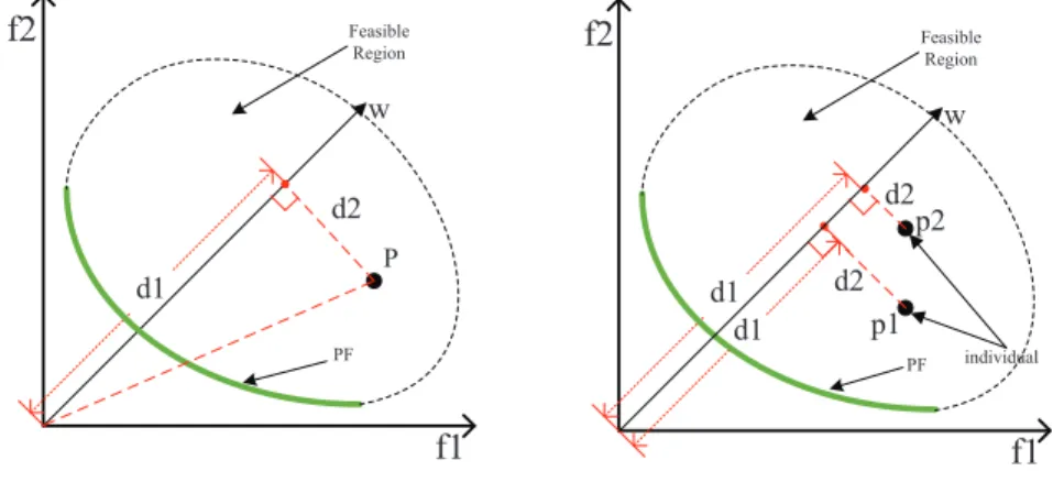
An example of an aggregate function value calculation is described in Figure 114
1. The d1 is Euclidean distance from perpendicular to the origin, and the d2
115
is Euclidean distance from perpendicular to the individual P. These parameters 116
f1
f2
d1 d2 P w PF Feasible RegionFigure 1: Illustration of the penalty-based boundary intersection approach in MOEA/D.
f1
f2
d2 d2 w p1 p2 d1 d1 individual PF Feasible RegionFigure 2: Illustration of the update operation.
can be computed respectively as follows: 117 d1= ||f(x)·wj|| ||wj|| . (1) d2=||f(x)−d1(wj/||wj||)||. (2) AF =d1+θ∗d2, (3)
where theθis set by the decision maker andAF is the aggregate function value
118
of the solution. It can be seen in Figure 2 that individualp1 will more likely be
119
replaced by individualp2 according to the aggregate function value, yet,p1 has
120
better convergence thanp2.
121
To solve this problem, we propose using the knee point selection strategy 122
instead of the aggregate function value strategy. This effectively prevents the 123
optimal solution from being replaced by the inferior solution. The knee point is 124
the most critical point on the PF. There are many methods to choose the knee 125
point. For example, you can see a knee point selection based on the angle[32] 126
in Figure 3. Slopes of the two lines through an individual and its two neighbors 127
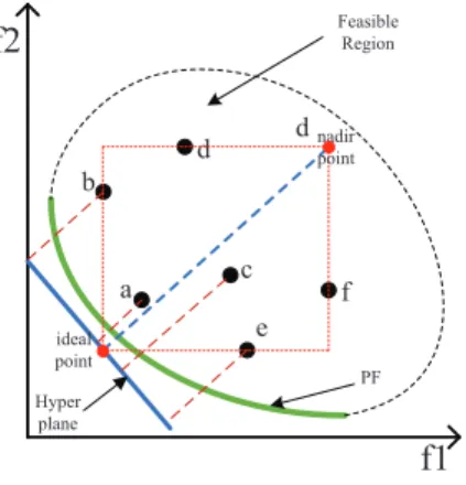
f1
a b c d e PF Feasible Regionf2
a © ©b ©c ©d ©eFigure 3: Illustration for determining knee point by angle for a bi-objective minimiza-tion problem.
f1
f2
PF Feasible Region a b d c f e Hyper plane d ideal point nadir pointFigure 4: Illustration for determining knee point by distance for a bi-objective minimiza-tion problem.
are shared, and then the angle between these slopes is regarded as a criterion 128
of whether the individual is at a knee or not. It is obvious that the angleθd is
129
the largest among all of the angles, so solution dis chosen as the knee point.
130
Another method for selecting knee points is based on the distance from the 131
point to hyperplane [33]. Using the ideal point and nadir point to construct a 132
hyperplane, the vertical distance of all solutions to the hyperplane is calculated. 133
The solution with the shortest vertical distance is chosen as the knee point. 134
Take two objective problems as an example, such as Figure 4, the solution with 135
the shortest distance will be the knee point. 136
Of the aforementioned methods, the first uses the angle of the adjacent 137
solution on both sides, meaning it cannot be applied to MaOPs because adjacent 138
angles are unsure. Thus, we choose the latter as the way to calculate the knee 139
point. In the KnEA [33], the knee point is selected from solutions of the same 140
Pareto layer. The solutions around the knee point are eliminated until all knee 141
points of the same Pareto layer are found. Even though the region exclusion 142
method is adopted, the population still easily falls into the marginal region. 143
This method can make full use of the solution’s convergence, but the diversity 144
f1
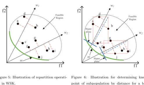
f2
w1 w2 a b c d f g h i j PF Feasible RegionFigure 5: Illustration of repartition operati-on in WSK.
f1
f2
w1 w2 a b c d f g h i j PF Hyper plane Hyper plane Feasible RegionFigure 6: Illustration for determining knee point of subpopulation by distance for a bi-objective minimization problem.
is not as good as the former. 145
In order to maximize the performance of the knee point, this paper proposes 146
an algorithm to introduce the concept of knee point to subpopulation. The 147
distance from solution to weight is computed to associated solution with weight. 148
In every subpopulation, the line through an ideal point and a nadir point is used 149
to construct a hyperplane. The distance from solution to hyperplane can be 150
regarded as a criterion of whether the individual is at a knee or not. As in Figure 151
5 and Figure 6, the whole population is divided into a set of subpopulations, and 152
the knee point is found in every subpopulation. We can see each subpopulation 153
has its own standard for calculating knee point rather than the unified formula 154
of MOEA/D. 155
3. PROPOSED ALGORITHM: WSK
156
The key task of WSK is to find the knee point of the subpopulation. As in 157
[33], the subpopulation knee point can be defined as follows: 158
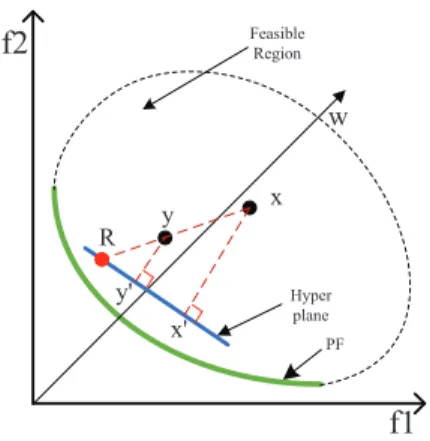
Definition of subpopulation knee point: An individual is considered 159
to be a knee point if and only if it has the shortest vertical distance from the 160
f1
f2
w Feasible Region x' x y y' R Hyper plane PFFigure 7: Illustration of the uniqueness of the knee point in the subpopulation.
individual to the hyperplane among the subpopulation. 161
According to this definition, the subpopulation’s knee point has the following 162
properties: 163
Property: If xis the knee point, it cannot be Pareto-dominated by other 164
individuals in the subpopulation. 165
Proof: Let us use a specific example shown in Figure 7 to prove this defini-166
tion. Supposexis knee point andy Pareto-dominates x. Connecting xandy,
167
it can be seen that vertical lineyy0 is parallel with vertical linexx0. According
168
to the similarity theorem of triangles,Ryy0 ∼Rxx0 (TriangleRyy0 is similar to
169
TriangleRxx0). Since Ry < Rx, we can derive thatyy0 < xx0. Obviously, the
170
result contradicts the hypothesis. Therefore, the property is reasonable. 171
3.1. General Framework of the Proposed Algorithm 172
The general framework of WSK consists of three parts: (1) Initialization, 173
which mainly aims to initialize a population; (2) Mating selection, which is to 174
selectN individuals for evolutionary operations through the binary tournament
175
selection. (In binary tournament selection, three criteria are adopted, namely, 176
the dominance relationship, the knee point judge and the crowding degree.) (3) 177
Environmental selection, which selects N individuals as the parent population of 178
the next generation. This procedure is repeated until the termination condition 179
is satisfied and the pseudocode of the general framework of WSK is shown in 180
Algorithm 1.
Algorithm 1General Framework of WSK
Input: P(population), W(weight)
Output: Ptmax 1: Initialization(P, W) 2: whileT < Tmaxdo 3: P = Mating selection(P) 4: Q= Variation(P) 5: Environmental selection(P, P , W) 6: T++ 7: end while 181 3.2. Mating Selection 182
The binary tournament selection has three competitive strategies. First, two 183
solutions are randomly chosen from the population. If one solution dominates 184
the other solution, the former is chosen. If there is no dominance relation
185
between the two solutions, individuals are checked to see whether they are knee 186
points or not. If one solution is a knee point and the other solution is not, 187
the former is chosen; otherwise, a third strategy is used. Next, the crowding 188
degrees between the two individuals are compared, and the bigger one was is 189
selected. The crowding degree is the sum of the angles between the solution and 190
the nearest two individuals. Finally, if the above conditions are all invalid, a 191
solution will be chosen randomly. The pseudocode of mating selection is shown 192
in Algorithm 2. 193
3.3. Environmental Selection 194
Environmental selection is to select solutions to form the next generation 195
of the population. Unlike other MOEAs with a nondominated sort, WSK does 196
Algorithm 2M ating Selection(P)
Input: P(population)
Output: Q(childpopulation)
1: Q← ∅
2: while|Q|<|N|do
3: randomly choose a and b f rom P
4: if a≺b then
5: Q←Q∪ {a}
6: else if b≺athen
7: Q←Q∪ {b}
8: else
9: if a.judgekneeistrue and b.judgekneeisf alsethen
10: Q←Q∪ {a}
11: else if b.judgekneeistrue and a.judgekneeisf alsethen
12: Q←Q∪ {b}
13: else
14: if a.crowd > b.crowdthen
15: Q←Q∪ {a} 16: else 17: Q←Q∪ {b} 18: end if 19: end if 20: end if 21: end while
not use nondominated sorting but elite replacement. The elite replacement
197
strategy is to replace the original population with the elite solutions of the 198
new population. Beforeenvironmental-selectionoperation, some strategies are
199
used. Normalization is used to compress the population into the standard space. 200
The repartition operation finds the nearest weight through min angle between 201
solution and weight. Hyperdistance represents the performance of a solution. 202
The details of environmental selection of WSK are presented in Algorithm 3.
Algorithm 3Environmental Selection(P, P0, W)
Input: P(population), N(populationsize), Q(archive)
Output: P(thenewpopulation) 1: i= 1 2: N ormalization(P0) 3: Repartition(P0, W) 4: ComputeHyperdistance(P0, W) 5: whilei <|W|do 6: U pdateP opulation(P, P0, W i) 7: i+ + 8: end while 9: if |P|>|W|then 10: Reduction(P) 11: end if 203
1) Normalization: The procedure of normalization is shown in Algorithm4.
First, the ideal pointZmin= (zmin1 , z
min
2 , . . . , z
min
m ) and nadir pointZmax=
(z1max, z2max, . . . , zmmax) are found, where theZminandZmaxdenote the
min-imal and maxmin-imal objective values in each objective function, respective-ly. Then the solutions in the populations are normalized to standard space through the following formula:
fi0(xj) =
fi−Zimin
Zmax
i −Zimin
, i= 1,2, . . . , m. (4)
Here thefi0(xj) is the transformed objective value.
204
2) Repartition: After the transformation of objective space, the repartition operation can be executed in transformed objective space. The angle between solution and weight are used to find the nearest weight of each solution in the population. The formula for calculating angles is as follows:
cosθ= Fi(x)·Wj(x) |Fi(x)| · |Wj(x)|
Algorithm 4N ormalization(P)
Input: P(population)
1: Calculate the minimal objective valueZmin , whereZimin=min
|P| j=1fi(xj),
i=1,2, . . . , m.
2: Calculate the minimal objective valueZmax , whereZimax=max
|P| j=1fi(xj),
i=1,2, . . . , m.
3: forj= 1 toP do
4: fori= 1 toM do
5: fi0(xj) = (fi−Zimin)/(Zimax−Zimin)
6: end for
7: end for
Here Fi(x)·Wj(x) return the inner product betweenFi(x) andWj(x). The
205
angle value is between zero and one. This procedure is shown in Algorithm5. 206
Algorithm 5Repartition(P, W)
Input: P(population), W(weightvector)
1: fori= 1 to|P|do 2: forj= 1 to|W|do 3: cosθ= Fi(x)·Wj(x) |Fi(x)|·|Wj(x)|, i= 1,2, ..., m 4: end for 5: end for
3) Compute Hyperdistance: The computation of hyperdistance is executed in 207
each subpopulation. By computing the direction of the ideal point and nadir 208
point, the normal vector of the hyperplane can be obtained. The solution 209
in the subpopulation needs to be calculated by taking the distance from the 210
point to hyperplane and the distance from the point to normal vector. The 211
sum of the two distances is used to indicate fitness value. 212
4) Update Population: The new population and original population need not be 213
merged, but the old population is updated by the new population. We need 214
to compare the distribution of new and old populations on the same weight. 215
If there is a solution assigned to this weight in the new population, but not 216
in the old population, the solution in the new population will be added. If 217
the old and new populations have solutions assigned to the same weight, the 218
best solution of the new population will replace the worst solution of the old 219
population. The superiority or inferiority of a solution is expressed by the 220
sum of hyperdistance and vertical distance between solution and weight. In 221
addition to the above two cases, other situations do not take any action.
Algorithm 6U pdateP opulation(P, P , W)
Input: P(population), W(weightvector)
1: fori= 1 to|W|do 2: if d(Wi).size= 0then 3: P =P∪P0(Wi) 4: else 5: forj= 1 to|P0(W i)|do
6: if P0.best betterthan P.worstthen
7: swap(P0.best, P.worst)
8: end if
9: end for
10: end if
11: end for
222
5) Reduction: After the update of the population, the size of the old population 223
may exceed the size required, so we need a reduction operation to reduce 224
some solutions in the population. To begin with, the extreme solutions in 225
each population are eliminated. Then, many solutions assigned to the same 226
weight are reduced. This prevents a knee point with poor performance and 227
extreme hyperdistance. 228
3.4. Computational Complexity Analysis 229
In this section, we show the analysis of the computational complexity of the 230
algorithms mentioned in this paper. We use the complexity within one iteration 231
Algorithm 7Reduction(P)
Input: P(population), W(weightvector)
1: while|P|>|W|do
2: Find theexS in P
3: reduceexS
4: end while
5: while|P|>|W|do
6: Calculate the maximal number ofd(Wi)
7: Reduce worst individual ind(Wi)
8: end while
as the complexity of the algorithm. For a population size N and
optimiza-232
tion problem of M objectives, the repartition operation has time complexity
233
O(M N2). Finding the ideal point and nadir point require a total of O(M N)
234
computations. The update operation has a time complexity of O(M N2). For
235
computing the operation of hyperdistance, a runtime of O(M N) is needed.
236
Therefore, the overall complexity of one generation in WSK is O(M N2).
Com-237
pared with recent popular MaEAs, the computational complexity of WSK is 238
considerable. 239
3.5. Discussion 240
In MOEA/D, NSGA-III and WSK, each population member is associated 241
with a reference line based on the perpendicular distance that could be measured 242
by angles to some extent. Notably, both ways consider the relation between the 243
individual and the reference line, which has no obvious difference in validity and 244
performance. 245
Consider the neighborhood concept. MOEA/D makes full use of the neigh-246
bor’s information, but the probability that the population falls into the local 247
optima increases. Different from MOEA/D, which uses a scalar function to 248
measure the convergence of a solution, WSK introduces the concept of a sub-249
population knee point, where the subpopulation knee point represents the best 250
convergence in the subpopulation. Meanwhile, one of the major differences be-251
tween the two algorithms is that WSK does not convert a MOP into a number 252
of scalar optimization subproblems. In NSGA-III, the perpendicular distance 253
between the individual and the reference line is served as either convergence or 254
diversity. Therefore, the NSGA-III has more difficulty converging than other 255
algorithms. 256
Unlike other algorithms such as KnEA and NSGA-III, which are based on 257
the nondominated sort, WSK uses elite replacement. The elite replacement 258
strategy replaces the original population with the elite solutions of the new 259
population. The subpopulation knee point used in WSK is different from KnEA. 260
Even though it has the same calculation method, the subpopulation knee point 261
is defined for each subpopulation and each one is unique, while the knee point 262
in KnEA is defined for the whole population and the number of knee points 263
increases with the evolution. 264
4. SIMULATION RESULTS
265
In this section, the performance of WSK is verified experimentally. We
266
compared WSK with seven state-of-the-art MaEAs for MaOPs, namely, S-267
PEA2+SDE [18], MOEA/D [22], MSOPS [20], NSGA-III [26], GrEA [16], HypE 268
[23] and KnEA [33] on the WFG [34], DTLZ [35] and ZDT [36] test suites. 269
4.1. Experimental Setting 270
For fairness, general parameters are used in this paper. Parameters were set 271
as follows: 272
1) Crossover and Mutation: The recommended SBX [37] and polynomial mu-273
tation [38] were adopted to generate offspring. The distribution index nc
274
of crossover was set to 20, and the crossover probability pc was set to 1.0.
275
Similarly, the distribution indexnm of mutation was set to 20, and the
mu-276
tation probabilitypmwas set to 1/n, wherendenotes the number of decision
277
variables. 278
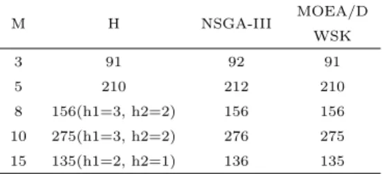
Table 1: Setting of population size M H NSGA-III MOEA/D WSK 3 91 92 91 5 210 212 210 8 156(h1=3, h2=2) 156 156 10 275(h1=3, h2=2) 276 275 15 135(h1=2, h2=1) 136 135
2) Population Size: The strategy of two-layered reference points in NSGA-279
III[26] was adopted to generate a set of uniformly distributed weight vectors. 280
Table 1 shows the setting of population size in MOEA/D and NSGA-III. 281
3) Number of Runs and Termination Condition: All algorithms were indepen-282
dently run 30 times on each test instance according to the parameter condi-283
tions. The setting of maximum function evaluations (MFEs) can be seen in 284
Table II. For different numbers of objectives, the termination condition can 285
be calculated byTmax= MFE/N.
286
4.2. Performance Metrics 287
In our experiment, two quality indicators were adopted to compare the per-288
formance of different algorithms. Both Inverted Generational Distance(IGD) 289
[39] and Hypervolume (HV) [40] can provide the information of convergence 290
and distribution of the algorithm simultaneously, have been accepted by peers 291
and are used as a common measure of algorithm performance evaluation. 292
1) IGD: This metric represents the mean distance between the solution on the 293
true PF and the nearest solution in the population. Let P be a set of points 294
uniformly distributed on the true PF, andP0 be a set of points in the
pop-295
ulation. For IGD, the smaller value is preferable, which indicates that the 296
solution set is close to the true PF and has a good distribution. The IGD 297
metrics are defined as follows: 298 IGD= 1 |P0| X z∈P0 dist(z, P). (6)
2) HV: This metric calculates the volume between the solution in the population 299
and the given reference point. A key issue that must be addressed to calculate 300
the HV indicator is the choice of the reference point. The objective value of 301
the population is normalized into the standard space according to the range 302
of the problems’ PFs. Similarly, the reference point is set to 1.1 times the 303
upper bound of the true PFs. We used Monte Carlo sampling[23] to evaluate 304
the performance of the algorithms. For HV, the bigger value is preferable. 305
To have statistically comprehensive conclusions, the Wilcoxon’s Rank test[41] 306
at a 0.05 significance level was adopted to test the significant difference between 307
the data obtained by paired algorithms. 308
4.3. Results and Analysis 309
The WFG test suite [34] is a set of widely used benchmark problems. These 310
test problems have various properties, such as having a concave, convex, mixed, 311
discontinuous, or degenerate PF and having a multimodal, biased or deceptive 312
search space. HV results in terms of the mean and standard deviation of the 313
MaEAs are shown in Table 2. As can be seen from the table, WSK performed 314
outstanding on all test problems except for WFG1. WFG1 has a mixed PF 315
and a biased search space. For WFG1, the performance of WSK is general and 316
SDE achieved the best HV value on all numbers of objectives. This occurrence 317
may be because the mixed PF affects the selection of the subpopulation knee 318
point. WFG2 has a convex and discontinuous PF. For WFG2, WSK achieved 319
the best HV values on 8-objective and 10-objective problems and achieved the 320
second best HV value on 3-objective and 5-objective problems. WFG3 has a 321
degenerate PF. WSK performs better than other algorithms on WFG2 with all 322
numbers of objectives except for 3. 323
For the other problems, different algorithms have their own strengths. Six 324
test problems, from WFG4 to WFG9 have a concave PF. For WFG4 and WFG8, 325
WSK obtained the best HV value on three test instances and obtained the sec-326
ond best HV value on three test instances. From the statistics, WSK is slightly 327
inferior to SDE and NSGA-III. For WFG5, WFG6, WFG7 and WFG9, WSK 328
performed better than the other algorithms. As we can see from the statistics, 329
WSK had excellent performance when dealing with asymmetric problems. 330
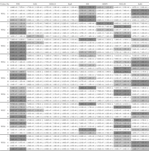
Table 2: HV (mean and standard deviation) results of the five algorithms on the WFG suites, where the best mean is shown with a deep gray background and the second best with a light gray background.
Problem Obj. WSK GrEA MOEA/D HypE SDE MSOPS NSGA-III KnEA
WFG1
3 4.088E+01 ( 7.27E-01 ) 4.774E+01 ( 2.12E+00 )∗4.557E+01 ( 2.39E+00 )∗4.010E+01 ( 1.33E+00 )‡5.133E+01 ( 2.53E+00 )∗5.042E+01 ( 1.81E+00 )∗4.648E+01 ( 2.55E+00 )∗4.927E+01 ( 2.93E+00 )∗ 5 3.359E+03 ( 6.44E+01 ) 3.796E+03 ( 6.13E+01 )∗3.973E+03 ( 1.17E+02 )∗3.222E+03 ( 1.21E+02 )‡4.272E+03 ( 1.39E+02 )∗4.210E+03 ( 1.12E+02 )∗4.219E+03 ( 7.96E+01 )∗4.274E+03 ( 1.97E+02) )∗ 8 1.107E+07 ( 1.66E+05 ) 1.047E+07 ( 1.36E+05 )∗1.146E+07 ( 2.79E+05 )∗9.201E+06 ( 1.41E+05 )‡1.397E+07 ( 6.19E+05 )∗1.081E+07 ( 1.38E+05 )‡1.102E+07 ( 4.01E+05 )†1.398E+07 ( 4.18E+05 )∗ 10 3.893E+09 ( 6.43E+07 ) 3.972E+09 ( 6.50E+07 )∗4.461E+09 ( 1.31E+08 )∗3.489E+09 ( 8.55E+07 )‡5.496E+09 ( 2.16E+08 )∗4.077E+09 ( 9.20E+07 )∗4.327E+09 ( 2.12E+08 )∗5.418E+09 ( 9.77E+09 )∗ 15 6.085E+16 ( 1.12E+15 ) 4.820E+16 ( 1.20E+15 )‡4.678E+16 ( 6.68E+14 )‡4.195E+16 ( 1.75E+15 )‡7.352E+16 ( 4.47E+15 )∗4.832E+16 ( 9.12E+14 )‡6.066E+16 ( 3.40E+15 )‡4.036E+16 ( 4.01E+17 )‡
WFG2
3 9.633E+01 ( 5.13E+00 ) 9.242E+01 ( 6.47E+00 )‡7.896E+01 ( 5.56E+00 )‡9.222E+01 ( 5.93E+00 )‡9.287E+01 ( 6.99E+00 )‡9.746E+01 ( 3.74E+00 )∗9.608E+01 ( 6.94E+00 )‡9.275E+01 ( 7.93E+00 )‡ 5 1.006E+04 ( 4.96E+01 ) 9.339E+03 ( 7.51E+02 )‡7.734E+03 ( 3.31E+02 )‡9.158E+03 ( 7.87E+02 )‡9.275E+03 ( 7.98E+02 )‡9.578E+03 ( 7.40E+02 )‡1.053E+04 ( 1.30E+01 )∗9.433E+03 ( 2.62E+02 )‡ 8 3.252E+07 ( 1.50E+06 ) 2.957E+07 ( 2.20E+06 )‡2.282E+07 ( 1.70E+06 )‡2.835E+07 ( 1.52E+06 )‡3.117E+07 ( 2.25E+06 )‡3.241E+07 ( 1.88E+06 )‡3.168E+07 ( 2.66E+06 )‡3.152E+07 ( 1.73E+06 )‡ 10 1.322E+10 ( 9.91E+08 ) 1.186E+10 ( 9.58E+08 )‡8.818E+09 ( 6.66E+08 )‡1.102E+10 ( 2.27E+08 )‡1.078E+10 ( 1.03E+09 )‡1.243E+10 ( 7.44E+08 )‡1.272E+10 ( 6.47E+08 )‡1.089E+10 ( 5.33E+08 )‡ 15 1.465E+17 ( 1.59E+16 ) 1.649E+17 ( 1.37E+16 )∗1.195E+17 ( 9.84E+15 )‡1.379E+17 ( 1.32E+16 )‡1.487E+17 ( 1.40E+16 )∗1.640E+17 ( 1.34E+16 )∗1.757E+17 ( 1.64E+16 )∗1.477E+17 ( 1.09E+17 )∗
WFG3
3 7.363E+01 ( 6.23E-01 ) 7.369E+01 ( 6.16E-01 )‡6.925E+01 ( 2.28E+00 )‡7.063E+01 ( 3.55E+00 )‡7.421E+01 ( 4.36E-01 )∗7.236E+01 ( 5.56E-01 )‡7.208E+01 ( 4.53E-01 )†7.396E+01 ( 4.24E+00 )∗ 5 6.599E+03 ( 2.49E+02 ) 6.471E+03 ( 1.37E+02 )‡5.836E+03 ( 1.98E+02 )‡3.367E+03 ( 7.84E+02 )‡6.163E+03 ( 2.13E+02 )‡6.443E+03 ( 8.40E+01 )‡6.344E+03 ( 4.56E+01 )‡6.173E+03 ( 3.97E+02 )‡ 8 2.010E+07 ( 2.47E+06 ) 1.864E+07 ( 6.89E+05 )‡1.288E+07 ( 1.39E+06 )‡3.231E+06 ( 2.01E+05 )‡1.945E+07 ( 8.68E+05 )‡1.717E+07 ( 5.46E+05 )‡1.960E+07 ( 1.42E+06 )‡1.971E+07 ( 8.44E+05 )† 10 8.236E+09 ( 2.16E+08 ) 6.669E+09 ( 7.80E+08 )‡3.200E+09 ( 9.00E+07 )‡9.606E+08 ( 8.22E+07 )‡7.492E+09 ( 3.40E+08 )‡6.589E+09 ( 1.82E+08 )‡7.815E+09 ( 8.29E+08 )‡7.256E+09 ( 9.48E+07 )‡ 15 9.298E+16 ( 1.60E+16 ) 8.196E+16 ( 8.89E+15 )‡1.808E+16 ( 1.11E+15 )‡1.083E+16 ( 2.26E+15 )‡8.587E+16 ( 1.07E+16 )‡8.055E+16 ( 5.02E+15 )‡7.575E+16 ( 1.29E+16 )‡8.536E+16 ( 7.42E+15 )‡
WFG4
3 7.510E+01 ( 4.00E-01 ) 7.382E+01 ( 3.30E-01 )‡7.126E+01 ( 7.60E-01 )‡7.093E+01 ( 3.12E+00 )‡7.501E+01 ( 4.22E-01 )†7.292E+01 ( 6.86E-01 )‡7.441E+01 ( 3.71E-01 )‡7.312E+01 ( 5.27E-01 )‡ 5 8.218E+03 ( 5.66E+01 ) 8.007E+03 ( 1.13E+02 )‡7.432E+03 ( 1.15E+02 )‡5.264E+03 ( 4.76E+02 )‡8.096E+03 ( 3.92E+01 )‡7.923E+03 ( 4.35E+01 )‡7.990E+03 ( 4.47E+02 )‡8.210E+03 ( 7.14E+00 )‡ 8 2.473E+07 ( 5.32E+05 ) 2.335E+07 ( 9.14E+05 )‡1.757E+07 ( 1.01E+06 )‡9.144E+06 ( 8.64E+05 )‡2.626E+07 ( 4.94E+05 )∗2.280E+07 ( 6.21E+05 )‡2.779E+07 ( 1.74E+06 )∗2.834E+07 ( 3.99E+05 )∗ 10 9.016E+09 ( 2.30E+08 ) 5.728E+09 ( 2.61E+08 )‡6.374E+09 ( 7.87E+08 )‡3.604E+09 ( 4.56E+08 )‡1.020E+10 ( 2.46E+08 )∗8.526E+09 ( 3.13E+08 )‡8.615E+09 ( 2.72E+08 )‡1.081E+10 ( 3.06E+08 )∗ 15 1.267E+17 ( 1.68E+15 ) 4.993E+16 ( 5.20E+15 )‡7.996E+16 ( 2.28E+16 )‡4.302E+16 ( 6.76E+15 )‡1.308E+17 ( 2.64E+15 )†8.077E+16 ( 5.17E+15 )‡1.425E+17 ( 5.22E+15 )∗1.404E+17 ( 9.65E+15 )∗
WFG5
3 7.210E+01 ( 4.88E-01 ) 7.051E+01 ( 3.34E-01 )‡6.926E+01 ( 5.82E-01 )‡7.013E+01 ( 3.06E+00 )‡7.204E+01 ( 6.01E-01 )†6.959E+01 ( 3.98E-01 )‡7.273E+01 ( 4.70E-01 )∗7.015E+01 ( 5.17E-01 )‡ 5 8.119E+03 ( 5.97E+01 ) 7.964E+03 ( 5.65E+01 )‡7.229E+03 ( 2.08E+02 )‡7.185E+03 ( 3.81E+02 )‡8.048E+03 ( 5.95E+01 )‡7.684E+03 ( 5.81E+01 )‡7.958E+03 ( 2.20E+01 )‡8.072E+03 ( 8.01E+01 )‡ 8 2.587E+07 ( 3.51E+05 ) 2.415E+07 ( 5.23E+05 )‡1.742E+07 ( 1.19E+06 )‡9.462E+06 ( 1.83E+06 )‡2.578E+07 ( 4.60E+05 )‡2.423E+07 ( 4.16E+05 )‡2.454E+07 ( 2.49E+06 )‡2.574E+07 ( 5.10E+05 )‡ 10 9.244E+09 ( 1.22E+08 ) 3.906E+09 ( 4.04E+08 )‡6.381E+09 ( 3.08E+08 )‡2.812E+09 ( 2.76E+08 )‡9.477E+09 ( 1.45E+08 )∗9.014E+09 ( 2.31E+08 )‡1.071E+10 ( 5.86E+08 )∗1.071E+10 ( 4.82E+07 )∗ 15 1.316E+17 ( 1.63E+15 ) 3.002E+16 ( 2.85E+15 )‡6.255E+16 ( 1.93E+15 )‡3.471E+16 ( 3.31E+15 )‡1.239E+17 ( 5.47E+15 )‡9.718E+16 ( 3.81E+15 )‡1.346E+17 ( 3.85E+15 )∗1.514E+17 ( 3.17E+14 )∗
WFG6
3 7.249E+01 ( 4.44E-01 ) 7.194E+01 ( 4.32E-01 )∗6.832E+01 ( 1.35E+00 )‡7.066E+01 ( 3.66E+00 )‡7.265E+01 ( 6.04E-01 )∗7.044E+01 ( 5.30E-01 )‡7.035E+01 ( 5.00E-01 )‡6.882E+01 ( 7.10E-01 )‡ 5 8.170E+03 ( 5.45E+01 ) 8.094E+03 ( 9.38E+01 )‡6.474E+03 ( 5.21E+02 )‡6.275E+03 ( 2.02E+02 )‡8.028E+03 ( 1.11E+02 )‡7.792E+03 ( 7.50E+01 )‡8.733E+03 ( 4.85E+01 )∗7.965E+03 ( 8.10E+01 )‡ 8 2.687E+07 ( 4.61E+05 ) 2.515E+07 ( 6.28E+05 )‡1.365E+07 ( 3.17E+05 )‡1.757E+07 ( 4.44E+06 )‡2.592E+07 ( 3.68E+05 )†2.568E+07 ( 7.17E+05 )‡3.076E+07 ( 3.16E+05 )∗2.634E+07 ( 4.94E+05 )‡ 10 1.276E+10 ( 3.32E+08 ) 4.024E+09 ( 2.92E+08 )‡4.595E+09 ( 9.12E+07 )‡3.033E+09 ( 5.59E+08 )‡1.069E+10 ( 2.27E+08 )∗9.897E+09 ( 1.64E+08 )∗8.959E+09 ( 6.30E+07 )‡1.112E+10 ( 2.87E+08 )‡ 15 1.479E+17 ( 6.90E+15 ) 2.967E+16 ( 3.91E+15 )‡6.070E+16 ( 2.21E+15 )‡2.084E+16 ( 8.43E+15 )‡1.391E+17 ( 5.03E+15 )‡1.169E+17 ( 4.25E+15 )‡1.331E+17 ( 6.75E+15 )‡1.419E+17 ( 2.20E+15 )‡
WFG7
3 7.574E+01 ( 2.86E-01 ) 7.492E+01 ( 2.72E-01 )‡6.921E+01 ( 2.04E+00 )‡7.393E+01 ( 2.59E+00 )‡7.608E+01 ( 4.55E-01 )∗7.327E+01 ( 5.74E-01 )‡7.435E+01 ( 4.51E-01 )‡7.432E+01 ( 2.05E+00 )‡ 5 8.702E+03 ( 6.72E+01 ) 8.577E+03 ( 7.42E+01 )‡7.112E+03 ( 2.50E+02 )‡7.428E+03 ( 3.78E+02 )‡8.553E+03 ( 5.73E+01 )‡8.255E+03 ( 8.83E+01 )‡9.186E+03 ( 2.78E+01 )∗8.682E+03 ( 3.39E+01 )‡ 8 2.695E+07 ( 6.87E+05 ) 2.592E+07 ( 6.43E+05 )‡1.494E+07 ( 6.95E+05 )‡1.430E+07 ( 2.31E+06 )‡2.528E+07 ( 4.32E+05 )‡2.572E+07 ( 6.91E+05 )‡2.213E+07 ( 4.51E+06 )‡2.571E+07 ( 8.00E+05 )‡ 10 9.827E+09 ( 2.15E+08 ) 5.455E+09 ( 1.93E+08 )‡5.852E+09 ( 7.23E+08 )‡4.435E+09 ( 1.14E+09 )‡9.762E+09 ( 3.68E+08 )‡8.874E+09 ( 4.22E+08 )‡6.786E+09 ( 9.02E+08 )‡1.005E+10 ( 9.48E+08 )∗ 15 1.525E+17 ( 4.57E+15 ) 4.675E+16 ( 4.29E+15 )‡6.672E+16 ( 1.65E+15 )‡3.760E+16 ( 4.74E+15 )‡1.456E+17 ( 4.89E+15 )‡7.536E+16 ( 9.35E+15 )‡1.462E+17 ( 1.82E+15 )‡1.524E+17 ( 4.77E+15 )†
WFG8
3 6.903E+01 ( 3.90E-01 ) 6.754E+01 ( 4.65E-01 )‡6.606E+01 ( 9.11E-01 )‡6.609E+01 ( 2.61E+00 )‡6.833E+01 ( 2.93E-01 )‡6.695E+01 ( 3.25E-01 )‡7.060E+01 ( 4.55E-01 )∗6.393E+01 ( 9.70E-01 )‡ 5 7.381E+03 ( 1.06E+02 ) 7.024E+03 ( 6.83E+01 )‡5.254E+03 ( 7.32E+02 )‡5.692E+03 ( 3.40E+02 )‡7.260E+03 ( 7.27E+01 )‡6.585E+03 ( 1.26E+02 )‡7.275E+03 ( 3.24E+02 )‡6.978E+03 ( 6.71E+01 )‡ 8 2.423E+07 ( 4.99E+05 ) 1.633E+07 ( 5.31E+05 )‡6.534E+06 ( 2.59E+06 )‡1.349E+07 ( 1.44E+06 )‡2.125E+07 ( 3.51E+05 )‡1.665E+07 ( 1.03E+06 )‡2.624E+07 ( 2.82E+06 )∗2.130E+07 ( 2.26E+06 )‡ 10 7.848E+09 ( 2.58E+08 ) 4.325E+09 ( 3.01E+08 )‡1.806E+09 ( 2.80E+08 )‡4.778E+09 ( 1.18E+09 )‡9.713E+09 ( 1.37E+08 )∗6.142E+09 ( 1.93E+08 )‡8.672E+09 ( 2.97E+08 )∗9.271E+09 ( 1.46E+09 )∗ 15 1.288E+17 ( 1.88E+15 ) 3.840E+16 ( 4.18E+15 )‡8.194E+16 ( 4.26E+16 )‡3.983E+16 ( 6.66E+15 )‡1.381E+17 ( 3.24E+15 )∗5.556E+16 ( 5.72E+15 )‡1.446E+17 ( 2.67E+15 )∗1.327E+17 ( 1.71E+17 )∗
WFG9
3 7.013E+01 ( 1.66E+00 ) 6.742E+01 ( 2.00E+00 )‡6.288E+01 ( 1.38E+00 )‡6.337E+01 ( 2.73E+00 )‡6.830E+01 ( 1.85E+00 )‡6.754E+01 ( 1.87E+00 )‡7.011E+01 ( 2.58E+00 )†6.668E+01 ( 2.06E+00 )‡ 5 7.500E+03 ( 7.74E+01 ) 7.411E+03 ( 1.79E+02 )‡6.490E+03 ( 7.45E+02 )‡6.189E+03 ( 3.62E+02 )‡7.311E+03 ( 2.01E+02 )‡6.836E+03 ( 9.44E+01 )‡7.444E+03 ( 1.91E+02 )‡7.222E+03 ( 1.90E+03 )‡ 8 2.263E+07 ( 9.97E+05 ) 1.949E+07 ( 1.19E+06 )‡1.077E+07 ( 3.73E+06 )‡1.083E+07 ( 2.08E+06 )‡2.254E+07 ( 6.53E+05 )‡1.771E+07 ( 1.55E+06 )‡2.508E+07 ( 1.31E+06 )∗2.541E+07 ( 7.62E+05 )∗ 10 8.386E+09 ( 4.35E+08 ) 4.700E+09 ( 3.77E+08 )‡4.859E+09 ( 1.39E+09 )‡3.152E+09 ( 6.97E+08 )‡8.567E+09 ( 4.27E+08 )∗5.853E+09 ( 5.99E+08 )‡8.616E+10 ( 2.60E+08 )∗9.435E+09 ( 4.80E+08 )∗ 15 1.140E+17 ( 4.41E+15 ) 4.439E+16 ( 3.79E+15 )‡2.693E+16 ( 1.28E+16 )‡3.819E+16 ( 7.03E+15 )‡1.110E+17 ( 3.95E+15 )‡5.944E+16 ( 9.88E+15 )‡1.058E+17 ( 2.84E+15 )‡1.124E+17 ( 1.11E+15 )‡ ‡indicates that the value is significantly outperformed by WSK
∗indicates that the value is significantly better than WSK
†indicates that no significant difference is detected.
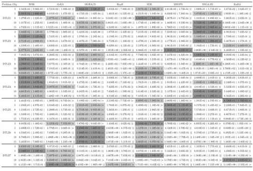
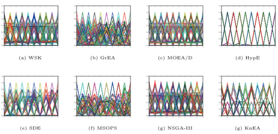
As in previous work, we compared the performance of these algorithms on 331
the seven DTLZ test problems in terms of IGD. From Table 3, some contrasting 332
results can be observed. WSK performed well on DTLZ2, DTLZ3 and DTLZ4. 333
For DTLZ1, WSK achieved the best IGD only on 5-objective problems. This 334
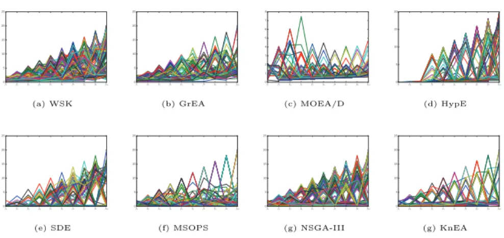
(a) WSK (b) GrEA (c) MOEA/D (d) HypE
(e) SDE (f) MSOPS (g) NSGA-III (g) KnEA
Figure 8: Final solution set of the seven algorithms on the 10-objective WFG9, shown by parallel coordinates.
Figure 9: Final solution set of the seven algorithms on the 5, 10, 15-objective WFG9, shown by box plots.
occurrence may be attributed to the flat PF. Although the subpopulation was 335
divided by weight, the calculation of the distance between the solution to the 336
hyperplane may still be affected by the PF. WSK achieved the best and sec-337
ond best IGD values on DTLZ2, DTLZ3 and DTLZ4. Among the DTLZ test 338
problems, DTLZ5 and DTLZ6 are considered to be degenerated problems. The 339
performance of WSK was general in DTLZ5 and DTLZ6. MOEA/D, SDE, M-340
SOPS and NSGA-III performed well on DTLZ5 and DTLZ6. This occurrence 341
may be attributed to the selection of the knee point. Although the knee point 342
represents the critical point in the subpopulation, the weight allocated on the 343
PF is very limited to degradation. For DTLZ7, WSK achieved the best IGD 344
value on 5 objectives and second best IGD value on 3 objectives. GrEA and 345
SDE performed well on DTLZ7. 346
Table 3: IGD (mean and standard deviation) results of the five algorithms on the DTLZ suites, where the best mean is shown with a deep gray background and the second best with a light gray background.
Problem Obj. WSK GrEA MOEA/D HypE SDE MSOPS NSGA-III KnEA
DTLZ1
3 2.345E-02 ( 9.96E-03 )3.721E-02 ( 1.09E-02 )‡ 1.866E-02 ( 2.02E-05 )∗ 5.835E-02 ( 7.88E-03 )‡ 1.947E-02 ( 2.58E-03 )∗2.813E-02 ( 4.75E-04 )‡1.920E-01 ( 5.71E-05 )∗ 3.875E-02 ( 3.04E-03 )‡ 5 5.391E-02 ( 1.88E-03 )6.835E-02 ( 1.47E-02 )‡ 6.175E-02 ( 1.63E-04 )‡ 1.401E-01 ( 6.53E-03 )‡ 6.231E-02 ( 5.94E-04 )‡8.036E-02 ( 7.26E-04 )‡ 5.876E-02 ( 1.34E-02 )‡1.903E-01 ( 1.38E+00 )‡ 8 1.279E-01 ( 1.22E-01 )1.077E-01 ( 7.89E-03 )∗ 1.088E-01 ( 6.39E-04 )∗3.610E+01 ( 2.52E+00 )‡8.695E-02 ( 1.80E-03 )∗1.267E-01 ( 8.75E-04 )†1.101E-01 ( 8.89E-02 )∗ 5.801E-01 ( 2.62E-01 )‡ 10 1.417E-01 ( 1.25E-02 )2.684E-01 ( 1.40E-01 )‡ 9.655E-02 ( 2.38E-04 )∗3.881E+01 ( 5.69E+00 )‡1.174E-01 ( 2.90E-03 )∗1.468E-01 ( 9.50E-04 )‡9.522E-02 ( 1.09E-01 )∗6.166E+00 ( 2.04E+00 )‡ 15 4.732E-01 ( 1.51E-02 ) 3.521E+01 ( 3.53E+01 )‡1.393E-01 ( 2.37E-03 )∗ 4.249E-01 ( 1.34E-01 )∗1.497E-01 ( 1.89E-03 )∗1.706E-01 ( 1.91E-03 )∗7.082E-02 ( 2.96E-01 )∗9.005E+00 ( 1.11E+01 )‡
DTLZ2
3 5.402E-02 ( 1.12E-04 )5.779E-02 ( 1.08E-03 )‡ 5.425E-02 ( 4.62E-06 )‡ 1.875E-01 ( 2.42E-02 )‡ 7.215E-02 ( 2.95E-03 )‡7.258E-02 ( 3.68E-04 )‡ 5.396E-02 ( 1.08E-04 )† 6.991E-02 ( 7.43E-02 )‡ 5 1.322E-01 ( 2.22E-04 )1.745E-01 ( 1.46E-03 )‡ 1.579E-01 ( 2.18E-04 )‡ 4.159E-01 ( 2.27E-02 )‡ 1.804E-01 ( 9.85E-03 )‡1.901E-01 ( 3.99E-03 )‡ 1.348E-01 ( 1.81E-03 )‡ 1.739E-01 ( 5.02E-01 )‡ 8 3.751E-01 ( 2.90E-03 )3.965E-01 ( 3.67E-03 )‡ 4.497E-01 ( 7.08E-04 )‡ 6.753E-01 ( 1.16E-02 )‡ 4.479E-01 ( 4.58E-03 )‡4.177E-01 ( 2.38E-03 )‡3.699E-01 ( 1.39E-03 )∗ 5.467E-01 ( 1.57E-01 )‡ 10 4.339E-01 ( 2.48E-03 )4.838E-01 ( 4.32E-03 )‡ 4.209E-01 ( 5.59E-04 )∗ 8.029E-01 ( 4.12E-02 )‡ 5.197E-01 ( 6.90E-03 )‡4.961E-01 ( 2.50E-03 )‡ 5.194E-01 ( 1.73E-01 )‡ 4.252E-01 ( 4.68E-03 )∗ 15 6.377E-01 ( 2.68E-03 ) 1.134E+00 ( 1.46E-01 )‡ 6.527E-01 ( 2.90E-02 )‡ 1.051E+00 ( 2.36E-02 )‡6.966E-01 ( 6.92E-03 )‡6.304E-01 ( 6.03E-03 )∗1.083E+00 ( 2.34E-02 )‡ 6.482E-01 ( 1.53E-02 )‡
DTLZ3
3 7.063E-02 ( 3.67E-03 )8.208E-02 ( 1.03E-02 )‡ 5.039E-02 ( 2.00E-04 )∗ 2.316E-01 ( 6.07E-02 )‡ 7.738E-02 ( 3.02E-03 )‡7.247E-02 ( 6.32E-04 )‡5.036E-02 ( 9.10E-05 )∗ 8.050E-02 ( 1.33E-04 )‡ 5 1.507E-01 ( 5.13E-03 )3.469E-01 ( 2.80E-01 )‡ 1.592E-01 ( 5.82E-04 )‡1.855E+02 ( 5.66E+01 )‡1.898E-01 ( 5.55E-03 )‡1.837E-01 ( 3.79E-03 )‡ 1.618E-01 ( 3.77E-02 )‡ 4.589E-01 ( 6.12E-02 )‡ 8 4.299E-01 ( 8.90E-03 )7.677E-01 ( 2.16E-01 )‡ 6.704E-01 ( 2.79E-01 )‡2.440E+02 ( 7.93E+00 )‡5.444E-01 ( 1.37E-02 )‡6.058E-01 ( 3.36E-01 )‡4.480E-01 ( 1.48E+00 )‡6.286E+01 ( 8.40E+00 )‡ 10 4.640E-01 ( 5.13E-03 )7.191E-01 ( 2.46E-01 )‡ 9.314E-01 ( 3.41E-01 )‡2.461E+02 ( 5.42E+00 )‡6.203E-01 ( 1.39E-02 )‡1.147E+00 ( 6.47E-01 )‡9.582E-01 ( 2.86E+01 )‡2.780E+02 ( 1.01E+02 )‡ 15 8.694E-01 ( 3.28E-02 ) 1.877E+02 ( 5.77E+01 )‡1.069E+00 ( 2.58E-01 )‡1.233E+02 ( 5.37E+01 )‡7.423E-01 ( 8.81E-03 )∗1.820E+00 ( 9.40E-01 )‡1.071E+00 ( 2.08E+01 )‡4.152E+02 ( 1.52E+02 )‡
DTLZ4
3 5.425E-02 ( 1.94E-01 )7.775E-02 ( 1.62E-03 )‡ 4.867E-01 ( 4.48E-01 )‡ 2.036E-01 ( 1.72E-01 )‡ 6.904E-02 ( 2.73E-01 )‡7.335E-02 ( 1.84E-04 )‡ 2.696E-01 ( 2.81E-01 )‡ 9.203E-02 ( 2.81E-03 )‡ 5 1.331E-01 ( 3.67E-04 )1.854E-01 ( 3.91E-02 )‡ 4.475E-01 ( 3.08E-01 )‡ 3.658E-01 ( 7.34E-02 )‡ 1.761E-01 ( 1.22E-01 )‡1.918E-01 ( 4.42E-03 )‡ 1.650E-01 ( 1.90E-01 )‡ 2.246E-01 ( 3.37E-03 )‡ 8 3.853E-01 ( 3.94E-03 )3.997E-01 ( 3.58E-03 )‡ 7.342E-01 ( 1.73E-01 )‡ 7.423E-01 ( 3.47E-02 )‡ 4.584E-01 ( 4.40E-02 )‡4.300E-01 ( 2.40E-03 )‡ 4.818E-01 ( 3.52E-01 )‡ 5.525E-01 ( 4.93E-03 )‡ 10 4.681E-01 ( 1.66E-03 )4.903E-01 ( 3.33E-03 )‡ 8.345E-01 ( 1.44E-01 )‡ 7.856E-01 ( 1.59E-02 )‡ 5.614E-01 ( 2.33E-02 )‡5.137E-01 ( 2.44E-03 )‡4.454E-01 ( 2.44E-01 )∗ 5.449E-01 ( 1.09E-02 )‡ 15 6.485E-01 ( 4.51E-04 ) 1.426E+00 ( 9.40E-02 )‡ 9.917E-01 ( 1.58E-01 )‡ 8.518E-01 ( 1.90E-02 )‡ 7.165E-01 ( 5.58E-03 )∗6.630E-01 ( 4.04E-03 )‡4.039E-01 ( 1.29E-01 )∗ 6.582E-01 ( 2.20E-03 )‡
DTLZ5
3 3.464E-02 ( 2.08E-03 )1.309E-02 ( 6.74E-04 )∗ 3.199E-02 ( 1.09E-04 )∗ 3.518E-02 ( 7.73E-03 )∗8.889E-03 ( 5.98E-04 )‡2.000E-02 ( 1.38E-04 )∗1.591E-02 ( 4.79E-03 )∗8.726E-03 ( 5.70E-03 )∗ 5 1.058E-01 ( 4.97E-02 )3.634E-02 ( 1.45E-02 )‡ 2.931E-02 ( 2.65E-04 )∗ 1.783E-01 ( 6.07E-02 )‡ 8.489E-02 ( 1.10E-02 )∗2.360E-02 ( 5.11E-03 )∗3.157E-02 ( 6.43E-02 )∗ 2.238E-01 ( 7.84E-01 )‡ 8 1.334E-01 ( 2.72E-02 )2.208E-01 ( 3.73E-02 )‡ 6.731E-02 ( 9.91E-05 )∗ 5.365E-01 ( 1.23E-01 )‡ 1.121E-01 ( 2.96E-02 )∗1.940E-02 ( 9.05E-03 )∗7.574E-01 ( 3.00E-01 )‡ 6.671E-01 ( 3.80E-01 )‡ 10 1.349E-01 ( 3.70E-02 )3.408E-01 ( 5.52E-02 )‡ 5.033E-02 ( 6.29E-03 )∗ 4.856E-01 ( 9.27E-02 )‡ 1.334E-01 ( 3.18E-02 )‡2.956E-02 ( 3.15E-02 )∗1.398E-01 ( 2.27E-01 )‡ 6.867E-01 ( 7.27E-01 )‡ 15 1.755E-01 ( 6.32E-02 )6.347E-01 ( 1.02E-01 )‡ 1.535E-01 ( 4.16E-05 )∗ 4.440E-01 ( 1.27E-01 )‡ 1.605E-01 ( 2.46E-02 )∗1.319E-01 ( 6.81E-02 )∗2.114E-01 ( 1.11E-01 )‡9.984E-01 ( 4.74E+00 )‡
DTLZ6
3 8.045E-02 ( 1.48E-02 )4.125E-02 ( 7.35E-03 )∗ 5.870E-02 ( 9.64E-03 )∗ 1.434E-01 ( 4.62E-02 )‡ 3.539E-02 ( 7.37E-03 )∗5.789E-02 ( 1.06E-02 )∗6.095E-02 ( 6.26E-03 )∗6.370E-02 ( 1.05E+01 )∗ 5 3.498E-01 ( 1.72E-02 )2.776E-01 ( 3.06E-01 )∗ 8.290E-02 ( 1.66E-02 )∗2.633E+00 ( 8.57E-02 )‡1.127E-01 ( 1.18E-02 )∗4.126E-01 ( 3.70E-02 )‡ 4.818E-01 ( 1.54E-01 )‡8.830E-01 ( 4.83E+00 )‡ 8 4.558E-01 ( 2.49E-02 )7.830E-01 ( 9.28E-01 )‡ 1.100E-01 ( 1.51E-02 )∗2.560E+00 ( 1.92E-01 )‡2.950E-01 ( 2.67E-02 )∗3.184E+00 ( 5.02E-01 )‡9.578E-01 ( 2.73E-01 )‡6.492E-01 ( 5.53E+00 )‡ 10 8.788E-01 ( 3.98E-02 ) 1.486E+00 ( 1.86E+00 )‡1.209E-01 ( 2.21E-02 )∗2.963E+00 ( 4.23E-01 )‡2.419E-01 ( 4.03E-02 )∗3.102E+00 ( 7.79E-01 )‡2.148E+00 ( 1.54E+00 )‡1.191E+01 ( 4.34E+01 )‡ 15 5.465E-01 ( 7.06E-02 ) 3.948E+00 ( 1.23E+00 )‡2.078E-01 ( 3.12E-02 )∗2.672E+00 ( 5.21E-01 )‡2.683E-01 ( 6.07E-02 )∗3.560E+00 ( 4.06E-01 )‡4.070E+00 ( 1.99E-01 )‡1.483E+00 ( 4.86E-02 )‡
DTLZ7
3 8.838E-02 ( 8.18E-02 )9.971E-02 ( 6.98E-03 )‡ 1.956E-01 ( 2.08E-01 )‡ 2.676E-01 ( 6.57E-02 )‡ 5.845E-02 ( 9.46E-02 )∗1.625E-01 ( 1.42E-02 )‡ 1.103E-01 ( 7.77E-02 )‡ 9.600E-02 ( 6.61E-01 )‡ 5 3.108E-01 ( 2.58E-02 )3.169E-01 ( 8.78E-03 )‡ 9.151E-01 ( 4.22E-01 )‡ 1.009E+00 ( 3.78E-01 )‡3.675E-01 ( 1.63E-02 )‡5.124E-01 ( 3.06E-02 )‡ 8.853E-01 ( 3.28E-01 )‡ 4.498E-01 ( 8.55E-02 )‡ 8 1.489E+00 ( 1.40E-01 ) 7.097E-01 ( 2.09E-02 )∗2.887E+00 ( 9.31E-01 )‡4.667E+00 ( 7.65E-01 )‡6.918E-01 ( 3.99E-02 )∗1.284E+00 ( 1.05E-01 )∗1.583E+00 ( 3.13E-01 )‡1.214E+00 ( 4.23E-02 )∗ 10 2.562E+00 ( 5.32E-01 ) 9.650E-01 ( 3.39E-02 )∗2.084E+00 ( 9.84E-01 )∗7.416E+00 ( 2.32E-01 )‡1.039E+00 ( 7.64E-03 )∗3.170E+00 ( 3.73E-01 )‡1.983E+00 ( 9.58E-01 )∗6.873E-01 ( 2.03E-02 )∗ 15 4.131E+00 ( 5.71E-01 ) 1.569E+00 ( 1.16E-01 )∗6.418E+00 ( 1.96E+00 )‡1.647E+00 ( 3.03E-01 )∗1.751E+00 ( 8.82E-02 )∗5.468E+00 ( 8.78E-01 )‡5.106E+00 ( 7.31E+00 )‡3.118E+00 ( 3.55E-01 )∗
To visualize the performance of algorithms in high-dimensional objective 347
space, the final solution set of the seven algorithms is shown by parallel coor-348
(a) WSK (b) GrEA (c) MOEA/D (d) HypE
(e) SDE (f) MSOPS (g) NSGA-III (g) KnEA
Figure 10: Final solution set of the seven algorithms on the 10-objective DTLZ2, shown by parallel coordinates.
Figure 11: Final solution set of the seven algorithms on the 5, 10, 15-objective DTLZ2, shown by box plots.
dinates. The lines with different colors represent different individuals in the 349
figure, so that information can be easily acquired by readers. Figure 8 shows 350
the final solution set of the WSK, GrEA, MOEA/D, HypE, SDE, MSOPS and 351
NSGA-III on the 10-objective WFG9. Clearly, for this problem, WSK has a set 352
of excellently distributed solutions over the PF; NSGA-III and SDE were slight-353
ly worse than WSK, and other algorithms were unable to maintain uniformity 354
in their solutions. Figure 10 gives the final solution obtained by WSK, GrEA, 355
MOEA/D, HypE, SDE, MSOPS and NSGA-III on the 10-objective DTLZ2. For 356
this problem, WSK and NSGA-III have a set of excellently distributed solutions 357
on the PF, HypE is unable to maintain uniformity of the solutions, and other 358
algorithms performed well in maintaining distribution. 359
Box plots are shown Figure 9 and Figure 11, where the plus sign represents 360
the extreme solution; the short line represents the range of all solutions; the red 361
line represents the mean value, and the rectangle represents the range of most 362
solutions except for the extreme solution. The smaller the rectangle is, the more 363
stable the algorithm is. In Figure 9 and Figure 11, WSK has a minimal rect-364
angle, indicating that WSK is a stable algorithm. In Figure 9, WSK achieved 365
a best mean value and best stability on the 5-objective and 15-objective prob-366
lems. NSGA-III achieved the best mean value on the 10-objective problems. 367
For DTLZ2, WSK obtained the best mean value on the 5-objective problem-368
s. MOEA/D obtained the best mean value on 10-objective problems. MSOPS 369
obtained the best mean value on 15 objectives. 370
From Table 2 and Table 3, we can see WSK achieved the best HV in eighteen 371
test instances and second best HV in twelve out of forty-five WFG test instances. 372
Furthermore, WSK achieved the best IGD in nine test instances and the second 373
best IGD in seven out of 35 DTLZ test instances. As a whole, WSK performed 374
better than the other algorithms. 375
As shown in tables 2 and 3, the best performance of WSK appears in the 376
problems DTLZ2-DTLZ4 and WFG4-WFG9. Specifically, WSK is good at these 377
kinds of problems. Although having various properties, these problems have the 378
same PF, which has a spherical shape. The reason for the better performance 379
Table 4: IGD (mean and standard deviation) results of the five algorithms on the ZDT suites, where the best mean is shown with a deep gray background and the second best with a light gray background.
Problem WSK GrEA MOEA/D HypE SDE MSOPS NSGA-III KnEA ZDT1 8.522E-02(2.14E-03) 1.899E-01(7.70E-03)‡ 1.203E-01(3.34E-04)‡5.246E-01(2.10E-03)‡8.679E-02(2.22E-03)‡8.492E-01(1.03E-01)‡5.674E-01(4.05E-02)‡ 2.765E-01(8.73E-03)‡
ZDT2 2.483E-01(3.70E-03) 4.605E-01(1.92E-02)‡ 4.225E-01(4.58E-02)‡6.339E-01(5.95E-03)‡4.092E-01(1.00E-02)‡1.149E+00(1.45E-01)‡1.112E+00(1.27E-01)‡4.254E-01(4.13E-02)‡
ZDT3 2.293E-01(4.91E-03) 1.776E-01(8.20E-03)∗ 1.565E-01(3.29E-03)∗4.947E-01(8.17E-03)‡1.054E-01(1.04E-03)∗8.377E-01(6.66E-02)‡4.132E-01(1.06E-01)‡ 2.472E-01(9.95E-03)‡
ZDT4 1.283E-01(1.74E-03) 2.410E-01(1.41E-02)‡ 5.739E-01(5.33E-02)‡6.245E-01(1.32E-02)‡1.280E-01(1.73E-03)∗9.009E-01(1.29E-01)‡4.825E-01(8.34E-02)‡ 3.374E-01(4.14E-02)‡
ZDT5 1.167E+00(4.85E-02) 3.173E+00(2.06E+00)‡7.897E+00(3.45E-03)‡2.350E+00(4.96E-02)‡1.013E+00(3.65E-02)∗1.456E+00(3.00E-01)‡1.026E+00(6.51E-02)∗6.075E+00(1.18E+00)‡
ZDT6 6.982E-02(3.27E-04) 1.610E-01(9.84E-04)‡ 1.050E-01(5.51E-04)‡8.552E-02(1.33E-03)‡7.022E-02(3.30E-04)†2.477E-01(9.67E-03)‡4.095E-01(3.18E-02)‡ 1.045E-01(2.27E-03)‡
of WSK on these test problems is that not only can the subpopulation knee 380
point ensure the direction of the search, but it can also dynamically adjust 381
the search direction of each subpopulation. What is more, the diversity and 382
convergence in WSK are kept balanced by update-population and reduction
383
operation. Meanwhile, this also may be attributed to the fact that the PFs of 384
the test problems are regular. To these problems, weight vectors cover the whole 385
PF regions, so the subpopulation knee point can take full advantage of its guide 386
function. Therefore, unlike NSGA-III and MOEA/D in which the directions are 387
fixed by weight vectors, WSK cannot be easily trapped into local optima. 388
Table 5: Statistical Result (mean and standard deviation) of the IGD value obtained by WSK* and WSK on DTLZ1 -DTLZ4,The best mean is shown with a deep gray background.
Problem Obj. WSK* WSK
DTLZ1
5 5.146E-02 ( 7.72E-09 ) 5.391E-02 ( 1.88E-03 )‡
10 8.100E-02 ( 1.65E-06 ) 1.417E-01 ( 1.25E-02 )‡
15 1.535E-01 ( 4.71E-06 ) 4.732E-01 ( 1.51E-02 )‡
DTLZ2
5 1.330E-01(1.89E-08) 1.322E-01 ( 2.22E-04 )‡
10 4.254E-01 ( 5.05E-06 ) 4.339E-01 ( 2.48E-03 )‡
15 6.356E-01 ( 4.19E-06 ) 6.377E-01 ( 2.68E-03 )‡
DTLZ3
5 1.340E-01 ( 8.95E-07 ) 1.507E-01 ( 5.13E-03 )‡
10 4.360E-01 ( 9.07E-06 ) 4.640E-01 ( 5.13E-03 )‡
15 6.465E-01 ( 2.21E-04 ) 8.694E-01 ( 3.28E-02 )‡
DTLZ4
5 1.499E-01(2.68E-03) 1.331E-01 ( 3.67E-04 )‡
10 4.540E-01 ( 1.38E-05 ) 4.681E-01 ( 1.66E-03 )‡
From Table 4, some contrasting results can be observed. WSK achieved 389
the best and second-best IGD values on ZDT1, ZDT2, ZDT4 and ZDT6. The 390
performance of WSK was general in ZDT3 and ZDT5. This occurrence may 391
be attributed to the discrete and discontinuous properties of the test problems. 392
In these problem, weight vectors have difficulty covering the whole PF regions 393
accurately, so the knee point cannot guide the population direction. 394
4.4. Discussion 395
To illustrate the performance of WSK, it was compared to six other state-396
of-the-art MaEAs on a series of test problems. The experimental results on test 397
problems with 3 to 15 objectives show that WSK is significantly better than 398
GrEA, MSOPS, and MOEA/D, and is comparative with SDE and NSGA-III. 399
In summary, given a large number of benchmark problems with various problem 400
characteristics and the performance metrics IGD and HV, WSK ensures better 401
performance in both convergence and diversity. 402
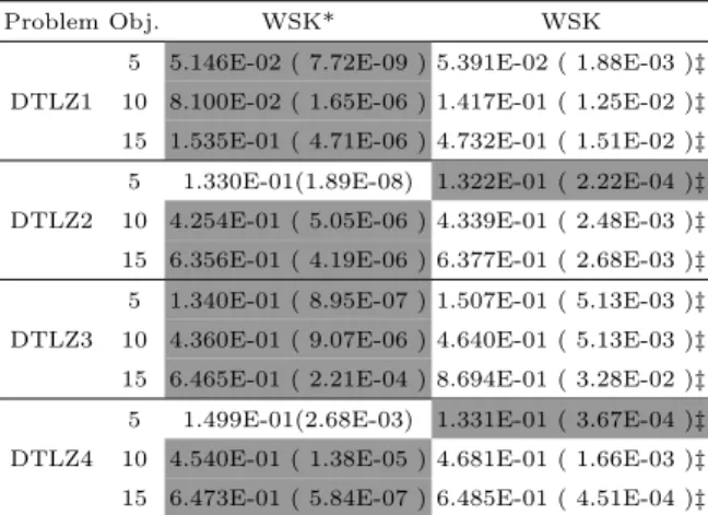
Meanwhile, the WSK with the normalization strategy removed (denoted as 403
WSK* hereafter) is compared with the original WSK. To compare the perfor-404
mance of the solutions obtained by WSK* and WSK, the IGD indicator is used. 405
As shown in Table 5, WSK* significantly outperformed the original WSK on 406
DTLZ1-4. The major reason for the better performance of WSK* on these 407
test problems is scaling of objective function. Since the association operation 408
of algorithm does not consider the scaling of individuals, the dimensions with 409
different scales will cause uneven distribution in the population. The accuracy 410
of the association operation will be reduced. 411
5. CONCLUSION
412
In order to ensure excellent convergence and diversity in solving MaOPs, this 413
paper has proposed an algorithm combining the advantages of decomposition 414
and knee point. In WSK, the worst solution of the old population was replaced 415
by the best solution in the new population. By repeating the update operation, 416
a solution set with good performance was obtained. 417
In addition, it is also worth mentioning that the performance of proposed 418
WSK is related to the shape of the PF for a given multiobjective problem since 419
a set of weights have different distributions on different shapes of PF. When 420
the shape of the PF is convex, the weight tends to be more concentrated on 421
the center of the PF; when the shape of the PF is concave, the weight tends 422
concentrate more on the edges of the PF. Therefore, WSK is not good at solving 423
convex problems because the number of solutions on the edge is difficult to 424
maintain. However, this problem can be addressed by adjusting each dimension 425
of weights (according to the extreme individual in the current population) before 426
the association operation. 427
In the next stage, we will have a deeper insight into the weight adjustment of 428
WSK, so as to further improve its performance. It would also be interesting to 429
extend our WSK to solve the problems with convex traits. Moreover, we would 430
apply WSK to real-world problems in order to further verify its effectiveness. 431
Studies on MOEAs have been carried out for many years. So far, many 432
MOEAs have been proposed. These algorithms have important guiding signif-433
icance for solving MOPs and practical research. In the study of MOEA, we 434
need to fully understand the idea of the algorithm and grasp its strengths and 435
weaknesses in order to provide a theoretical basis for further research. 436
6. Acknowledgements
437
The authors wish to thank the support of the National Natural Science 438
Foundation of China (Grant No. 61876164, 61502408, 61673331), the Education 439
Department Major Project of Hunan Province (Grant No. 17A212), The MOE 440
Key Laboratory of Intelligent Computing and Information Processing, the Sci-441
ence and Technology Plan Project of Hunan Province (Grant No. 2016TP1020), 442
the Provinces and Cities Joint Foundation Project (Grant No. 2017JJ4001), the 443
Hunan province science and technology project funds(2018TP1036). 444
References
445
[1] B. Li, J. Li, K. Tang, X. Yao, Many-objective evolutionary algorithms: A 446
survey, Acm Computing Surveys 48 (1) (2015) 13. 447
[2] G. Fu, Z. Kapelan, J. R. Kasprzyk, P. Reed, Optimal design of water dis-448
tribution systems using many-objective visual analytics, Journal of Water 449
Resources Planning & Management Asce 139 (6) (2013) 624–633. 450
[3] R. J. Lygoe, M. Cary, P. J. Fleming, A real-world application of a many-451
objective optimisation complexity reduction process. 452
[4] P. J. Fleming, R. C. Purshouse, R. J. Lygoe, Many-objective optimization: 453
An engineering design perspective, Lecture Notes in Computer Science 3410 454
(2005) 14–32. 455
[5] V. Khare, X. Yao, K. Deb, Performance scaling of multi-objective evolu-456
tionary algorithms, in: International Conference on Evolutionary Multi-457
Criterion Optimization, 2003, pp. 376–390. 458
[6] K. Deb, A. Pratap, S. Agarwal, T. Meyarivan, A fast and elitist multi-459
objective genetic algorithm: Nsga-ii, IEEE Transactions on Evolutionary 460
Computation 6 (2) (2002) 182–197. 461
[7] E. Zitzler, M. Laumanns, L. Thiele, Spea2: Improving the strength pareto 462
evolutionary algorithm. 463
[8] D. W. Corne, N. R. Jerram, J. D. Knowles, M. J. Oates, Pesa-ii: region-464
based selection in evolutionary multiobjective optimization, in: Conference 465
on Genetic and Evolutionary Computation, 2001, pp. 283–290. 466
[9] G. Ruan, G. Yu, J. Zheng, J. Zou, S. Yang, The effect of diversity mainte-467
nance on prediction in dynamic multi-objective optimization, Applied Soft 468
Computing 58 (2017) 631–647. 469
[10] J. Zou, Y. Zhang, S. Yang, Y. Liu, J. Zheng, Adaptive neighborhood selec-470
tion for many-objective optimization problems, Applied Soft Computing. 471
[11] J. Zou, J. Zheng, R. Shen, C. Deng, A novel metric based on changes in 472
pareto domination ratio for objective reduction of many-objective optimiza-473
tion problems, Journal of Experimental & Theoretical Artificial Intelligence 474
29 (5) (2017) 1–12. 475
[12] J. Zou, L. Fu, S. Yang, J. Zheng, G. Yu, Y. Hu, A many-objective evolu-476
tionary algorithm based on rotated grid, Applied Soft Computing 67. 477
[13] L. Fu, J. Zou, S. Yang, R. Gan, Z. Ma, J. Zheng, A proportion-based 478
selection scheme for multi-objective optimization, in: Computational Intel-479
ligence, 2018, pp. 1–7. 480
[14] D. Hadka, P. M. Reed, T. W. Simpson, Diagnostic assessment of the borg 481
moea for many-objective product family design problems, in: Evolutionary 482
Computation, 2012, pp. 1–10. 483
[15] H. Sato, H. E. Aguirre, K. Tanaka, Controlling Dominance Area of So-484
lutions and Its Impact on the Performance of MOEAs, Springer Berlin 485
Heidelberg, 2007. 486
[16] S. Yang, M. Li, X. Liu, J. Zheng, A grid-based evolutionary algorithm for 487
many-objective optimization, IEEE Transactions on Evolutionary Compu-488
tation 17 (5) (2013) 721–736. 489
[17] S. F. Adra, P. J. Fleming, Diversity management in evolutionary many-490
objective optimization, IEEE Transactions on Evolutionary Computation 491
15 (2) (2011) 183–195. 492
[18] M. Li, S. Yang, X. Liu, Shift-based density estimation for pareto-based 493
algorithms in many-objective optimization, IEEE Transactions on Evolu-494
tionary Computation 18 (3) (2014) 348–365. 495
[19] Y. Liu, D. Gong, S. Jing, Y. Jin, A many-objective evolutionary algorithm 496
using a one-by-one selection strategy, IEEE Transactions on Cybernetics 497
47 (9) (2017) 2689–2702. 498
[20] E. J. Hughes, Multiple single objective pareto sampling, in: Evolutionary 499
Computation, 2003. CEC ’03. The 2003 Congress on, 2004, pp. 2678–2684 500
Vol.4. 501
[21] T. Ray, M. Asafuddoula, A. Isaacs, A steady state decomposition based 502
quantum genetic algorithm for many objective optimization, in: Evolu-503
tionary Computation, 2013, pp. 2817–2824. 504
[22] Q. Zhang, H. Li, Moea/d: A multiobjective evolutionary algorithm based 505
on decomposition, IEEE Transactions on Evolutionary Computation 11 (6) 506
(2007) 712–731. 507
[23] J. Bader, E. Zitzler, Hype: An algorithm for fast hypervolume-based many-508
objective optimization, Evolutionary Computation 19 (1) (2014) 45–76. 509
[24] M. Emmerich, N. Beume, B. Naujoks, An emo algorithm using the hy-510
pervolume measure as selection criterion, in: International Conference on 511
Evolutionary Multi-Criterion Optimization, 2005, pp. 62–76. 512
[25] E. Zitzler, S. Knzli, Indicator-Based Selection in Multiobjective Search, 513
2004. 514
[26] K. Deb, H. Jain, An evolutionary many-objective optimization algorithm 515
using reference-point-based nondominated sorting approach, part i: Solv-516
ing problems with box constraints, IEEE Transactions on Evolutionary 517
Computation 18 (4) (2014) 577–601. 518
[27] B. Li, J. Li, K. Tang, X. Yao, An improved two archive algorithm for many-519
objective optimization, in: Evolutionary Computation, 2014, pp. 524–541. 520
[28] H. J. F. Moen, N. B. Hansen, H. Hovland, J. Trresen, Many-objective op-521
timization using taxi-cab surface evolutionary algorithm, in: International 522
Conference on Evolutionary Multi-Criterion Optimization, 2013, pp. 128– 523
142. 524
[29] Y. Xiang, Y. Zhou, M. Li, Z. Chen, A vector angle-based evolutionary algo-525
rithm for unconstrained many-objective optimization, IEEE Transactions 526
on Evolutionary Computation 21 (1) (2017) 131–152. 527
[30] H. K. Singh, A. Isaacs, T. Ray, A pareto corner search evolutionary algo-528
rithm and dimensionality reduction in many-objective optimization prob-529
lems, IEEE Transactions on Evolutionary Computation 15 (4) (2011) 539– 530
556. 531
[31] J. Zou, J. Zheng, C. Deng, R. Shen, An evaluation of non-redundant objec-532
tive sets based on the spatial similarity ratio, Soft Computing 19 (8) (2015) 533
2275–2286. 534
[32] J. Branke, K. Deb, H. Dierolf, M. Osswald, Finding knees in multi-objective 535
optimization (2004) 722–731. 536
[33] X. Zhang, Y. Tian, Y. Jin, A knee point-driven evolutionary algorithm for 537
many-objective optimization, IEEE Transactions on Evolutionary Compu-538
tation 19 (6) (2015) 761–776. 539
[34] S. Huband, P. Hingston, L. Barone, L. While, A review of multiobjective 540
test problems and a scalable test problem toolkit., IEEE Transactions on 541
Evolutionary Computation 10 (5) (2006) 477–506. 542
[35] K. Deb, L. Thiele, M. Laumanns, E. Zitzler, Scalable multi-objective opti-543
mization test problems, in: wcci, 2002, pp. 825–830. 544
[36] E. Zitzler, K. Deb, L. Thiele, Comparison of multiobjective evolutionary 545
algorithms: Empirical results, Evolutionary Computation 8 (2) (2000) 173– 546
195. 547
[37] K. Deb, R. B. Agrawal, Simulated binary crossover for continuous search 548
space 9 (3) (1994) 115–148. 549
[38] K. Deb, M. Goyal, A combined genetic adaptive search (geneas) for engi-550
neering design, 1996, pp. 30–45. 551
[39] Q. Zhang, A. Zhou, Y. Jin, RM-MEDA: A Regularity Model-Based Multi-552
objective Estimation of Distribution Algorithm, IEEE Press, 2008. 553
[40] L. While, P. Hingston, L. Barone, S. Huband, A faster algorithm for cal-554
culating hypervolume, IEEE Transactions on Evolutionary Computation 555
10 (1) (2006) 29–38. 556
[41] E. Zitzler, J. Knowles, L. Thiele, Quality assessment of pareto set approx-557
imations, in: Multiobjective Optimization, 2008, pp. 373–404. 558