Heuristic Rule Learning
Vom Fachbereich Informatik der Technischen Universität Darmstadt zur Erlangung des akademischen Grades eines Doktor der Naturwissenschaften (Dr. rer. nat.)
genehmigte
Dissertation
von
Dipl.-Inform. Frederik Janssen (geboren in Bad Schwalbach)
Referent: Prof. Dr. Johannes Fürnkranz Korreferent: Niklas Lavesson, Ph.D.
School of Computing,
Blekinge Institute of Technology Karlskrona, Sweden
Tag der Einreichung: 29.08.2012 Tag der mündlichen Prüfung: 10.10.2012
D17 Darmstadt 2012
Please cite this document as
URN: urn:nbn:de:tuda-tuprints-31352
URL: http://tuprints.ulb.tu-darmstadt.de/3135 This document is provided by tuprints,
E-Publishing-Service of the TU Darmstadt http://tuprints.ulb.tu-darmstadt.de [email protected]
Abstract
The primary goal of the research reported in this thesis is to identify what criteria are responsible for the good performance of a heuristic rule evaluation function in a greedy top-down covering algorithm both in classification and regression. We first argue that search heuristics for inductive rule learning algorithms typically trade off consistency and coverage, and we investigate this trade-off by determining op-timal parameter settings for five different parametrized heuristics for classification. In order to avoid biasing our study by known functional families, we also inves-tigate the potential of using metalearning for obtaining alternative rule learning heuristics. The key results of this experimental study are not only practical de-fault values for commonly used heuristics and a broad comparative evaluation of known and novel rule learning heuristics, but we also gain theoretical insights into factors that are responsible for a good performance. Additionally, we evaluate the spectrum of different search strategies to see whether separate-and-conquer rule learning algorithms are able to gain performance in terms of predictive ac-curacy or theory size by using more powerful search strategies like beam search or exhaustive search. Unlike previous results that demonstrated that rule learning algorithms suffer from oversearching, our work pays particular attention to the in-teraction between the search heuristic and the search strategy. Our results show that exhaustive search has primarily the effect of finding longer, but nevertheless more general rules than hill-climbing search.
A second objective is the design of a regression rule learning algorithm. To do so, a novel parametrized regression heuristic is introduced and its parameter is tuned in the same way as before. A new splitpoint generation method is introduced for the efficient handling of numerical attributes. We show that this metric-based algo-rithm performs comparable to several other regression algoalgo-rithms. Furthermore, we propose a novel approach for learning regression rules by transforming the regression problem into a classification problem. The key idea is to dynamically define a region around the target value predicted by the rule, and considering all examples within that region as positive and all examples outside that region as negative. In this way, conventional rule learning heuristics may be used for induc-ing regression rules. Our results show that our heuristic algorithm outperforms approaches that use a static discretization of the target variable, and performs en par with other comparable rule-based approaches, albeit without reaching the performance of statistical approaches.
In the end, two case studies on real world problems are presented. The first one deals with the problem of predicting skin cancer and the second one is about
decid-ing whether or not students have to be invited to a counseldecid-ing session. For reasons of interpretability, rules were perfectly suited to work with in both case studies. The results show that the derived rule-based algorithms are able to find rules that are very diverse, proved to be interesting, and are also sufficiently accurate. All experiments were performed in the SECO-Framework, a new versatile framework for heuristic rule learning, which allows for an easy configuration of a wide range of different components rule learners consist of.
Zusammenfassung
Das hauptsächliche Forschungsziel dieser Dissertation ist, Kriterien zu identifizie-ren, die für eine gute Performanz von heuristischen Evaluationsfunktionen in ei-nem Greedy Top-Down Covering Algorithmus verantwortlich sind. Dies wurde sowohl für Klassifikation als auch für Regression untersucht. Zu Beginn wird ar-gumentiert, dass Suchheuristiken für induktive Regel-Lern-Algorithmen typischer-weise zwischen Konsistenz und Abdeckung abwägen. Es werden Parameter für fünf verschiedene Heuristiken für Klassifikation zur optimalen Abwägung dieser beiden Ziele bestimmt. Diese Parameterwerte sind von praktischer Relevanz da sie als Standardwerte für Regel-Lern-Algorithmen verwendet werden können. Um aber eine Beeinflussung durch bereits bekannte Funktionsfamilien auszuschließen, wird das Potential von Meta-Lernverfahren untersucht, um alternative Regel-Lern-Heuristiken zu erhalten. Hervorzuheben ist, dass theoretische Einblicke in Fakto-ren, die für eine gute Performanz verantwortlich sind, in beiden Studien gewonnen wurden. Des Weiteren wurde das Spektrum verschiedener Suchstrategien ana-lysiert, um festzustellen ob Separate-and-Conquer Algorithmen von mächtigeren Suchstrategien wie z.B. einer Beam-Suche oder einer vollständigen Suche im Hin-blick auf Genauigkeit oder Theoriegröße profitieren können. Im Gegensatz zu bis-herigen Resultaten aus der Literatur, in welchen festgestellt wurde, dass Regel-Lern-Algorithmen am sog. „Oversearching“ leiden, wird in dieser Arbeit beson-deres Augenmerk auf das Zusammenspiel zwischen der Suchheuristik sowie der Suchstrategie gelegt. Die Ergebnisse verdeutlichen, dass eine vollständige Suche den vorrangigen Effekt hat längere, aber trotzdem generellere Regeln als eine Hill-Climbing Suche zu finden.
Ein zweites Ziel dieser Dissertation ist die Erstellung eines Regel-Lern-Algorithmus für Regression. Um dieses Ziel zu erreichen wird eine parametri-sierbare Regressionsheuristik entworfen und der Parameter wird in der gleichen Weise wie zuvor angepasst. Eine effiziente Methode um Splitpoints zu generieren wird ebenfalls eingeführt, da man auf aus der Klassifikation bekannte Verfahren nicht zurückgreifen kann. Es wird gezeigt, dass dieser Metrik-basierte Algorithmus vergleichbar gut wie andere Regressionsalgorithmen funktioniert, obwohl er ein deutlich simpleres Modell für die Regeln verwendet. Im Weiteren wird eine neuar-tige Methode präsentiert mit welcher Regressionsregeln gelernt werden können in-dem Regression in ein Klassifikationsproblem transformiert wird. Die Kernidee ist, dynamisch eine Region um den Vorhersagewert der Regel zu definieren, innerhalb dieser alle Beispiele als positiv zu betrachten sind und alle die außerhalb liegen als negativ. So können konventionelle Regel-Lern-Heuristiken verwendet werden, um
Regressionsregeln zu lernen. Die Experimente zeigen, dass der entwickelte heuris-tische Algorithmus signifikant bessere Ergebnisse als eine staheuris-tische Diskretisierung liefert. Zudem ist das Verfahren ähnlich gut wie andere regelbasierte Ansätze wenn auch nicht so gut wie statistische Methoden.
Zuletzt werden zwei Fallstudien präsentiert, die auf realen Daten durchgeführt werden. Das Ziel der ersten Studie ist das Hautkrebsrisiko eines Patienten vor-herzusagen. In der zweiten Studie geht es um die Entscheidung, ob Studieren-de entsprechend verschieStudieren-dener persönlicher Daten zu einem Beratungsgespräch eingeladen werden müssen. Aus Gründen der guten Interpretierbarkeit sind Re-geln optimal geeignet um diese beiden Probleme zu lösen. Die Resultate zeigen, dass die in dieser Dissertation eingeführten Regel-Lern-Algorithmen geeignet sind, Regeln zu finden die sehr unterschiedlich, die für Domänenexperten interessant und die trotzdem noch ausreichend genau sind. Alle Experimente wurden im sog. SECO-Framework durchgeführt, einem neuartigen vielseitigen Framework für heu-ristisches Regel-Lernen welches eine bequeme Konfiguration verschiedenster Kom-ponenten eines Regel-Lern-Algorithmus erlaubt.
Acknowledgements
This thesis was done at theKnowledge Engineering Groupat the TU Darmstadt. The whole research presented was supported by theGerman Science Foundation (DFG). Without this support this work would not have been possible.
In the beginning, I would like to thank Prof. Dr. Johannes Fürnkranz for his support during my time at the Knowledge Engineering Group. He always had an open ear for all the problems that arose through the years. Not only in scientific topics but also in all other questions he provided a constant support. Without all the discussions with him I never would have had the opportunity to finish such a thesis. Prof. Dr. Johannes Fürnkranz also provided a fruitful environment to do research, namely the Knowledge Engineering Group. I am very glad that I had the opportunity to work under his supervision and I could not imagine a better support. Secondly, I like to thank my second supervisor Associate Prof. Niklas Lavesson, PhD. Niklas and I met at theSDMconference in 2009 and quickly recognized that we are both interested in very similar research topics. I am glad that he accepted to review my thesis and I am thankful for all the high quality comments he made. He clearly participated in improving the thesis considerably.
I am also thankful to Prof. Dr. Mira Mezini, Prof. Dr. Chris Biemann, and Prof. Dr. Ulf Brefeld for being part of the board of examiners.
During my time at the Knowledge Engineering Group I had the opportunity to work with very funny but also very smart colleagues. I never had the feeling that I am not totally satisfied to be able to work in this group. We always had fun, even in times when there was a lot to do and the atmosphere was not as pleasant as usual. In particular, I like to thank Dr. Eneldo Loza Mencía for many fruitful discussions (also during several vacations), Dr. Sang-Hyeun Park for being my cigarette partner during the time I was a smoker (I quit smoking now) and the interesting conversations, Dr. Heiko Paulheim for introducing me to the Semantic Web and for writing papers with me, Jan-Nikolas Sulzmann for working on the same project as I, and Lorenz Weizsäcker for interesting discussions (from every point of view). I also wish to thank all the student workers who supported my thesis by implementing the main parts of the SECO-Framework or by working on several other important topics. During the years Raad Bahmani, David Schuld, and Markus Zopf supported the framework and my work. Dirk große Osterhues and Kilian Kiekenap provided working hardware so that all experiments could be conducted very conveniently. I never could forget to mention the secretary Gabriele Ploch. I would like to thank her for all the nice chats during breaks and all the good tips for a whole bunch of different things.
In the end, I would like to thank my parents Uta Janssen and Peter Janssen. With-out them nothing at all could have been possible in my whole life. They always supported me in every aspect a child could wish for. My father even introduced me to Computer Science in the first place. Without him I would have never found such joy in working on topics concerned with computational problems. My father and I had the chance of being part of the early days of the information age and even loaded the first programs by playing a cassette. I am very glad that my mother al-ways was there for me and supported me with everything one can imagine. I never had to bother with anything related to my education because it was always clear that a constant support is ensured. I also like to thank my brother Arik Janssen for all the interesting discussions away from all the computer science topics. Life has much more to offer than sitting in front of a computer which my brother constantly highlighted. Walter Untermann was there for me any time I needed him, so I am also very grateful for that. I like to thank Golriz Chehrazi who supported me most of the time during my job as a PhD-guy.
Many thanks go to my girlfriend Martina Hochstatter. She never hesitated to proof-read the thesis even when I tried to convince her that this really is not neces-sary. The mistakes and typos she found in my thesis are uncountable as her support for me and my love for her also is.
Contents
1 Introduction 1
1.1 Contributions . . . 2
1.2 Contents . . . 4
2 Inductive Rule Learning 7 2.1 Foundations of Machine Learning and Inductive Rule Learning . . . . 8
2.1.1 Classification . . . 10
2.1.2 Regression . . . 11
2.2 Separate-and-Conquer Rule Learning . . . 12
2.2.1 Introduction of Rules . . . 13
2.2.2 A straight-forward Separate-and-Conquer Algorithm . . . 15
2.2.3 Searching for good Rules . . . 17
2.2.4 Discussion of the straight-forward Algorithm . . . 18
2.2.5 Characterizing Separate-and-Conquer Algorithms . . . 19
2.3 Handling Multi-Class Problems . . . 20
2.3.1 (Unordered) 1-vs-all Class Binarization . . . 21
2.3.2 Ordered 1-vs-all Class Binarization . . . 22
2.3.3 Pairwise Class Binarization . . . 24
2.3.4 Ordered and Unordered Lists of Rules . . . 25
2.4 Overfitting Avoidance . . . 27
2.5 Visualization with Coverage Space Isometrics . . . 29
2.6 Rule Learning Heuristics . . . 30
2.6.1 Basic Heuristics . . . 32
2.6.2 Composite Heuristics . . . 33
2.6.3 Parametrized Heuristics . . . 36
2.6.4 Gain-Heuristics . . . 39
2.7 Evaluation Methods for Rule Learning Algorithms . . . 40
2.7.1 Cross-Validation . . . 40
2.7.2 Theory size . . . 41
2.7.3 Evaluation of Regression Rule Learning Algorithms . . . 42
2.7.4 Evaluation of Classification Rule Learning Algorithms . . . 44
2.7.5 Evaluation of Performance Rankings . . . 45
3 The SECO-Framework for Rule Learning 49
3.1 Separate-and-conquer Rule Learning in the SECO-Framework . . . 49
3.2 Unifying Rule Learners in the SECO-Framework . . . 53
3.2.1 Fixed Properties of the SECO-Framework . . . 54
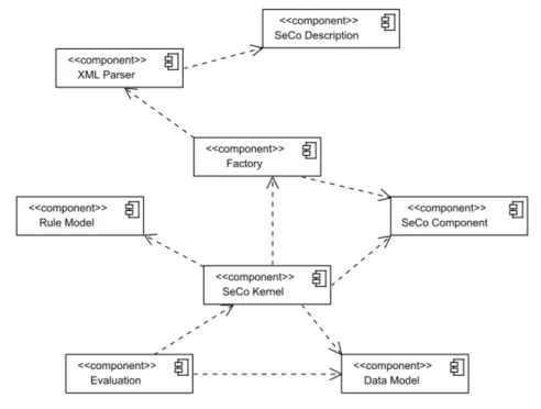
3.3 Architecture of the SECO-Framework . . . 56
3.4 Configurable Objects in the Framework . . . 58
3.4.1 Binarization in the SECO-Framework . . . 61
3.5 Example Configurations . . . 63 3.5.1 CN2 . . . 64 3.5.2 AQ . . . 64 3.5.3 RIPPER . . . 65 3.5.4 SIMPLESECO . . . 68 3.6 Evaluation Package . . . 70 3.7 Related Work . . . 73 3.8 Summary . . . 75
4 Heuristics for Classification 77 4.1 Experimental Setup . . . 79
4.1.1 The Datasets . . . 81
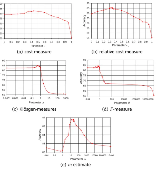
4.2 Optimization of Parametrized Heuristics . . . 81
4.2.1 Search Strategy . . . 81
4.2.2 Optimal Parameters for the Five Heuristics . . . 83
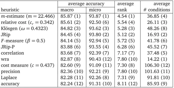
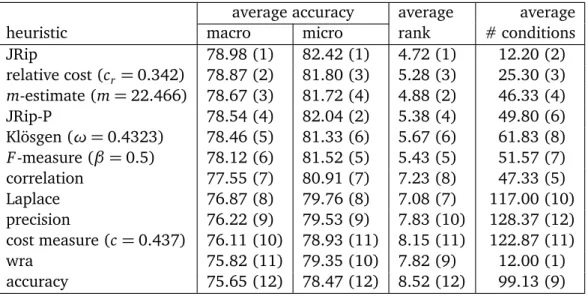
4.2.3 Experimental Results of the Tuned Heuristics . . . 84
4.2.4 Interpretation of the Learned Heuristics . . . 91
4.3 Meta-Learning of Rule Learning Heuristics . . . 91
4.3.1 Meta-Learning Scenario . . . 92
4.3.2 Experimental Results . . . 95
4.3.3 Interpretation of the Learned Functions . . . 100
4.4 Related Work . . . 103
4.5 Summary . . . 105
5 A Comparison of Search Algorithms for Heuristic Rule Learning 107 5.1 Implementation of the Algorithm . . . 108
5.2 Search Strategies . . . 108 5.2.1 Hill-Climbing . . . 109 5.2.2 Beam Search . . . 109 5.2.3 Exhaustive Search . . . 110 5.3 Experimental Setup . . . 111 5.4 Results . . . 113
5.4.1 Varying the Beam Size . . . 113
5.4.2 Single Rules . . . 115
5.4.4 Runtime of the Search Methods . . . 120
5.5 Bidirectional Rule Learning . . . 120
5.5.1 Theoretical Considerations . . . 121 5.5.2 Experimental Setup . . . 122 5.5.3 Results . . . 123 5.5.4 Discussion . . . 127 5.6 Related work . . . 128 5.7 Summary . . . 129
6 A Metric-Based Approach to Regression Rule Learning 131 6.1 Separate-and-Conquer Rule Learning for Regression . . . 132
6.2 Regression Datasets, Regression Algorithms, and Experimental Setup 133 6.3 A Direct Adaption of the SIMPLESECORule Learner to Regression . . . 135
6.3.1 Splitpoint Processing . . . 137
6.4 Optimizing Several Parameters . . . 139
6.4.1 Splitpoint and Left-Out-Parameter . . . 140
6.4.2 Parameter of the Regression Heuristic . . . 142
6.5 Results . . . 144
6.5.1 Using Different Numbers of Splitpoints . . . 144
6.5.2 Comparison with other Systems on the Tuning Datasets . . . . 145
6.5.3 Comparison with other Algorithms on the Test Sets . . . 147
6.6 Related Work . . . 149
6.7 Summary . . . 150
7 Regression via Dynamic Reduction to Classification 151 7.1 Dynamic Reduction to Classification . . . 152
7.2 Experimental Setup . . . 154
7.3 Results . . . 156
7.4 Comparison of Metric-Based Algorithms and Dynamic Reduction . . . 159
7.5 Related Work . . . 161
7.6 Summary . . . 162
8 Experiments on Real-World Data 165 8.1 Using Rule Learning Algorithms to Predict Skin Cancer . . . 165
8.1.1 Introduction to the domain . . . 166
8.1.2 The datasets . . . 168
8.1.3 Results . . . 171
8.2 Using Rule Learning to Identify Students Who Need Assistance . . . . 175
8.2.1 Introduction to the domain . . . 176
8.2.2 The dataset . . . 177
8.2.3 Results . . . 179
8.4 Summary . . . 183
9 Discussion of the Results 185 10 Conclusions and Future Work 191 10.1 Conclusions . . . 191
10.2 Future Work . . . 195
10.2.1 SECO-Framework . . . 195
10.2.2 Classification Heuristics . . . 195
10.2.3 Search Algorithms . . . 196
10.2.4 Regression Rule Learning . . . 196
10.2.5 Real-World Applications . . . 197
Bibliography 199
List of Figures
2.1 Comparison of a rule set and a linear regression . . . 12
2.2 A4-class classification problem . . . 21
2.3 1-vs-all class binarization . . . 22
2.4 The second step of an ordered class binarization . . . 23
2.5 Two steps of a pairwise class binarization . . . 24
2.6 A simple decision list . . . 26
2.7 A strongly overfitted rule set . . . 27
2.8 Isometrics in 2-d and 3-d coverage space . . . 29
2.9 Isometrics forrecallandMinNegCoverage. . . 32
2.10 Isometrics forprecision . . . 34
2.11 Isometrics forcorrelation. . . 35
2.12 General behavior of the F-Measure . . . 37
2.13 Klösgen-Measure for different settings ofω . . . 38
3.1 Example of a refinement process . . . 51
3.2 UMLdiagram of the SECOstructure . . . 55
3.3 UMLdiagram of the SECOcomponents . . . 56
3.4 UMLdiagram of the SECOdata model . . . 57
3.5 UMLdiagram of the SECOheuristics . . . 58
3.6 XMLconfiguration of CN2 . . . 63
3.7 XMLconfiguration of AQ . . . 64
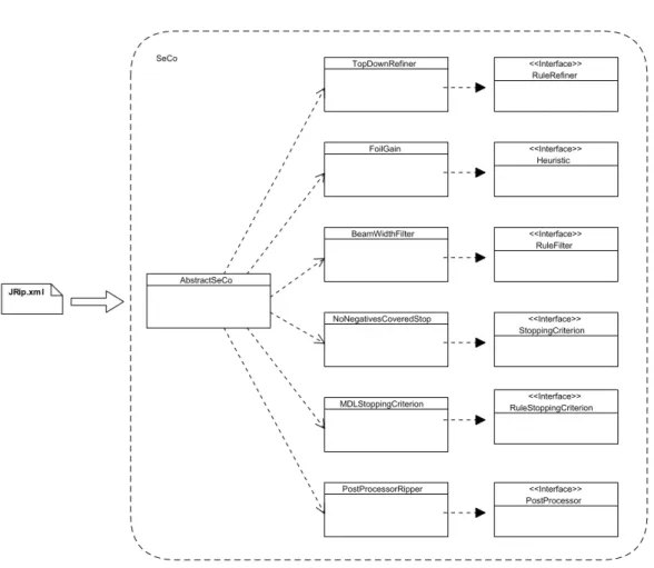
3.8 XML-configuration of RIPPER . . . 65
3.9 UMLof RIPPERimplemented in the SECO-Framework . . . 66
3.10 XMLconfiguration of SIMPLESECO . . . 69
3.11 Property-file of an evaluation configuration . . . 71
4.1 Accuracy over parameter values for five parametrized heuristics . . . 82
4.2 Comparison of all heuristics with the Nemenyi test . . . 88
4.3 Isometrics of the best parameter settings . . . 90
4.4 Histogram of frequencies . . . 97
4.5 Isometrics of three meta-heuristics . . . 102
5.1 Hill-Climbing and Beam Search . . . 109
5.2 Ordered Exhaustive search . . . 110
5.3 Accuracy and number of conditions vs. beam size . . . 112
5.5 Bidirectional search, based on [95] . . . 121
6.1 Example of the splitpoint clustering method . . . 136
6.2 Parameters overrrmsefor both subsets of the tuning datasets . . . 141
6.3 Isometrics of the regression heuristic forα=0.59 . . . 143
6.4 Comparison of the algorithms on the two subsets . . . 146
7.1 Comparison of the algorithms from Table 7.2 with the Nemenyi test . 157 7.2 Comparison of the algorithms from Table 7.3 with the Nemenyi test . 161 8.1 Selected rules on datasetD1 . . . 172
8.2 Selected rules on datasetD2 . . . 173
8.3 Selected rules on datasetD3 . . . 174
List of Algorithms
2.1 SEPARATEANDCONQUER(Examples) . . . 15
2.2 FINDBESTRULEWITHTOPDOWNSEARCH(Examples) . . . 16
3.1 ABSTRACTSECO(Examples) . . . 50
3.2 FINDBESTRULE(Growing, Pruning) . . . 52
4.1 GENERATEMETADATA(TrainSet,TestSet), adapted from [57] . . . 93
List of Tables
2.1 A sample classification task . . . 10
2.2 A sample regression task . . . 11
2.3 The confusion matrix . . . 17
2.4 Basic heuristics . . . 32
2.5 Composite heuristics . . . 33
2.6 Parametrized heuristics . . . 36
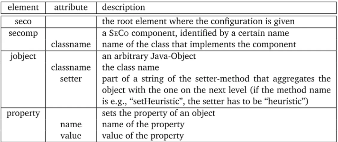
3.1 Elements and attributes of a SECOdescription inXML . . . 59
3.2 Combination of the binarization method and classification method . . 62
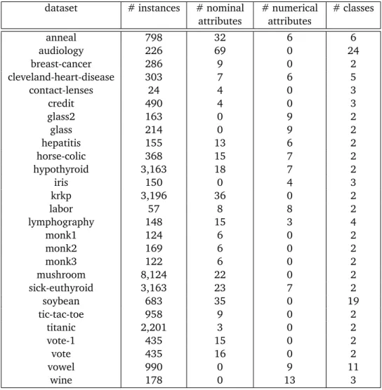
3.3 The17datasets used for experiments with the optimization phase . . 67
3.4 Fields of the evaluation . . . 72
4.1 The 27 tuning datasets . . . 79
4.2 The 30 validation datasets . . . 80
4.3 Results of the optimal parameter settings on the 27 tuning datasets . 85 4.4 Results of the optimal parameter settings on the 30 validation datasets 86 4.5 Spearman rank correlation for Table 4.3 and 4.4 . . . 86
4.6 Win/Loss/Tie Statistics and thep-values on the 30 validation datasets 87 4.7 Accuracy of the five heuristics when used in JRIPand CN2 . . . 89
4.8 Accuracies of SIMPLESECOfor several meta-learned heuristics . . . 96
4.9 Accuracies of SIMPLESECOfor two meta-learned heuristics . . . 98
4.10 Comparison of heuristics for training set and predicted coverages . . 99
4.11 Coefficients of various functions learned by linear regression . . . 100
5.1 Number of rules/conditions for hill-climbing and exhaustive search . 115 5.2 Results for the single rule learner . . . 116
5.3 Runtimes (in sec.) of the heuristics with different beam sizes . . . 119
5.4 Results of the top-down and the bidirectional approach . . . 123
5.5 Comparison of RIPPERand bidirectional search . . . 125
5.6 Comparison of bidirectional and beam search forcorrelation. . . 126
5.7 Comparison of bidirectional and beam search form-estimate . . . 127
6.1 Overview of the tuning databases for regression . . . 133
6.2 Overview of the validation databases for regression . . . 134
6.3 Results for the splitpoint computation and left-out-parameter . . . 140
6.5 Runtime of different splitpoint methods on the test set . . . 144
6.6 Results for different algorithms on the tuning datasets . . . 145
6.7 Results in terms ofrrmsefor differentWekaalgorithms on the test set 147 6.8 Comparison to REGENDER on some of the test datasets . . . 148
7.1 Evaluation of dynamic and static regression and rule-based learners . 155 7.2 Comparison of bagged version and other algorithms . . . 158
7.3 Comparison of the two approaches including other algorithms . . . . 159
8.1 The attributes given by the patient and by the dermatoligist . . . 167
8.2 Statistics of the three datasets . . . 168
8.3 Theory size and performance of differentWekaalgorithms . . . 170
8.4 Different statistics for selected configurations of SIMPLESECO. . . 171
8.5 The44attributes used for prediction . . . 177
1 Introduction
With the emergence of the Internet and computer systems that have more and more storage space, the available information also grows drastically. Nowadays, there are estimates that 15 Petabyte of new information are generated every day [74]. Clearly, the process of extracting valuable knowledge, whatever form it may have, becomes unfeasible for a human. Consequently, computer systems are neces-sary that are able to extract important knowledge out of the mass of information. The task of finding relationships in datasets is called data mining. Data mining involves methods ofmachine learning. Machine learning focuses on the design and construction of algorithms that are able to learn. The discipline of machine learn-ing, however, is a branch of artificial intelligence, which dates back to 1956when John McCarthy coined the term when he wrote a proposal for the Darthmouth Summer Research Project on Artificial Intelligence1. Today, there are many differ-ent subfields of machine learning [117] such as neural networks, support vector machines, or rule learning.
The latter is the main topic of this thesis. The discipline of rule learning dates back to the early days of the field of machine learning. It has various subfields such as association rule mining (see for example [1, 77, 102]), inductive logic pro-gramming (see [120, 121, 136]), and propositional rule learning. We are mostly concerned with the task ofpropositionalorattribute-valuerule learning, where the rules are learned from a single table. The most famous strategy for learning such decision rules is the so-calledseparate-and-conquerorcovering strategy. This strat-egy was proposed in 1969 by Ryszard S. Michalski [113]. The discipline of rule learning had its up and downs but research on this topic never completely van-ished. The main reason to foster research on models that are composed by simple, interpretable rules is that they are easy to understand. Hence, a human has the ability to comprehend what a rather incomprehensible algorithm has learned on a given set of information. This property is not evident for most of the machine learning algorithms. In fact, one might argue that only decision trees are also interpretable by humans.
Especially in domains where the experts are unfamiliar with machine learning, algorithms that yield interpretable models are beneficial. Often, humans also think in a more or less rule-based way [140] which makes it easy to compare knowledge, because, at least to some extent, it is built in a similar manner. The advantages then are that these simple models are more trustful in the eyes of an expert, that they 1 The full proposal can be found under http://www-formal.stanford.edu/jmc/history/
can be compared to the assumptions of the humans, and that faulty parts of the model can be detected easily. In this sense, rules provide an excellent testbed for interacting with fields different from machine learning.
Through the years considerable progress had been made in the field of rule learn-ing. Various authors proposed an amazing number of different algorithms. Never-theless, rule learning is hard to analyze from a statistical point of view due to its combinatorial complexity or the heuristic search (cf. [144]). Following from this, there are different aspects of rule learning that are still not well researched. For ex-ample, the requirements of rule learning heuristics are still not framed in a unifying way. Despite, there is some work on providing theoretical frameworks for analyz-ing heuristics [60]. But still, some fundamental issues of heuristics are not well known. For example, it is unclear which parameter setting works best for heuris-tics that feature a parameter. While there are some suggestions (cf. [180, 96, 97] for the Klösgen-Measure ), a solid empirical evaluation is yet missing for other mea-sures. Presumably, a single parameter setting that works best in all situations can also not be found because of the no free lunch theorem [179]. Essentially, the the-orem states that an optimal setting always is domain-dependent. It is also an open question how heuristics behave when different search algorithms are employed. Albeit there is some work (cf. [134]), this topic needs to be further examined. For the task of regression, some heuristics were proposed but there is also a lack of clear formulations, which requirements heuristics should met in this field. How different heuristics behave when the same algorithm is used has yet to be investi-gated in detail. Often, only some heuristics are evaluated for a certain algorithm. A comprehensive overview still needs to be done. This thesis can be seen as an approach to answer some of these questions.
Interestingly, most of the rule learning algorithms share several concepts. For ex-ample, the majority of decision rule learning algorithms are based on the separate-and-conquer strategy. In spite of these similarities, there is no unifying framework in which, for example, different algorithms based on the same basic strategy could be implemented. Often, new work about an algorithm can be characterized as changing some of the fundamental elements of the algorithm (cf., e.g., the im-provements of CN2 [20, 19]). Thus, such a unifying framework would be of great value for the rule learning community. It is also a necessary first step to ease the experiments conducted in this work.
1.1 Contributions
In this thesis the following contributions are made. General framework for rule learning
To unify different rule learning algorithms, the SECO-Framework for rule learning is introduced (note that SECOstands for Separate-and-Conquer). The framework
al-lows to configure rule learning algorithms by specifying different building blocks. In this way, it is easy to interchange the components of a given algorithm. The modular design allows to implement many existing rule learning algorithms and simplifies the process of changing components of one algorithm such as the heuris-tic or the search algorithm. Due to an evaluation package that is included in the SECO-Framework, comparing several algorithms is also a simple task.
Broad understanding of heuristics for classification
The work reported in this thesis enriches the general understanding of the heuris-tic component most rule learning algorithms consist of. For some parametrized heuristics for classification, optimal parameters are suggested based on an em-pirical optimization. Beyond that, two entirely new heuristics are derived and compared to existing ones. It is shown that their performance is comparable to the best heuristics for classification. Another important insight is that the prefer-ence structure of those heuristics is also quite similar to existing state-of-the-art heuristics.
Rule learning algorithms for regression
For the task of regression, on the one hand, a novel heuristic to solve regression directly is derived and evaluated. On the other hand, by the usage of a reduc-tion scheme, the performance of classificareduc-tion heuristics for regression is reported. Thus, two algorithms that are able to deal with numerical target attributes are developed. The evaluation shows that their performance is comparable to other regression algorithms. Besides, the limitations that come with the rule based ap-proach to regression are also discussed in detail.
Schemes for reducing regression to classification
A new mechanism to dynamically reduce the regression problem to classification is introduced. Among the interesting observations when using the reduction is that heuristics that are known to find many rules in classification end up in considerably fewer rules when used in regression. The scheme is not restricted to rule learning but can also be employed whenever an algorithm is based on positive and negative coverage statistics (as, e.g., decision tree algorithms are).
Behavior of heuristics in different search scenarios
Most of the research about classification heuristics deals with scenarios where the search algorithm of the rule learner is fixed. The majority of systems only use a simple hill-climbing search instead of complex search algorithms. The work re-ported here contributes to the understanding of how the requirements of heuristics change when they are used in more complex search algorithms. The performance of algorithms that employ these elaborate search algorithms, scaled even up to a true exhaustive search, is evaluated with a special focus on the phenomenon of oversearching.
1.2 Contents
In Chapter 2 the separate-and-conquer strategy, which forms the basis for most algorithms used in this thesis, is illustrated on the basis of two simple algorithms. Separate-and-conquer rule learning is used to solve the concept learning problem which is also described. When more than two classes are present, means for re-ducing the data to two-class problems are discussed. The main tool for a graphical analysis of heuristics, the so-called coverage space, is introduced. Subsequently, some general concepts for the design of rule learning heuristics are summarized. Then, the different rule learning heuristics that are used in this thesis are intro-duced. For some of them, examples of their isometrics in coverage space are also given. The chapter concludes with a descriptionn of evaluation methods for classi-fication and regression rule learning algorithms.
Chapter 3 gives an overview of the SECO-Framework for rule learning, a new versatile and extendable framework. The architecture and the components are described. The chapter is completed by showing how to implement some existing algorithms in the framework and by a brief description of an additional evaluation package that is part of the framework.
In Chapter 4 work on classification heuristics is reported. It starts with a sum-mary on the research on parameter tuning of heuristics. The parameters of five heuristics are optimized. The heuristics are compared by using the coverage space framework. In the following, new heuristics are derived that are learned by a meta-learning approach. The chapter also includes an extensive empirical evaluation.
Chapter 5 deals with the search algorithm of the rule learning algorithm. Based on a previous work on that topic [134], in this chapter the experiments are ex-tended. The focus lies on the behavior of different classification heuristics, includ-ing those tuned in the previous chapter, when the search algorithm is changed. In particular, simple hill-climbing, beam search, a true exhaustive search, and a bidirectional search are compared against each other and against state-of-the-art algorithms.
Heuristics for regression are described in Chapter 6. The chapter summarizes work on a direct adaption of the classification algorithm to regression. Conse-quently, a new heuristic for regression had to be designed and some additional changes to the basic algorithm are described. The new algorithm is compared against other well-known algorithms.
Chapter 7 deals with a different approach to regression. Here, a mechanism to dynamically reduce the regression problem to classification is presented. As a consequence of the reduction, the heuristics for classification from Chapter 4 can be used again. In the end of the chapter, a comparison of the two regression algorithms is given.
In Chapter 8 experiments on real-world data are shown. The main purpose here is to demonstrate that the derived algorithms also perform well on actual
data. All previous experiments were done on datasets that are publicly available in repositories. These datasets may not meet the conditions that are observed in real-world data. For this reason, two domains were picked and experiments on the derived datasets are reported.
Chapter 9 focuses on providing a unified view of separate-and-conquer rule learning algorithms. Here, all results and observations are put into context fol-lowing some identified criteria a good rule learning heuristic has to fulfill.
2 Inductive Rule Learning
Inductive learningis the process of deriving a general description from special cases in an empirical way. Its direct counterpart is deduction where special cases are de-rived from general given knowledge. Generalizations from specialized cases are constructed in the form of a model. This model can then be applied on new pre-viously unseen cases and is able to categorize them. Often, when some form of assignments of cases to certain categories or classes is been employed in an au-tomated way, this is referred to as classification. Classification is the process of constructing a definition of a class. Among others, this can be achieved by the
concept learningapproach.
Concept learning was introduced by Bruner, Goodnow, and Austin [10] in1967
and is defined there as “the search for and listing of attributes that can be used to distinguish exemplars from non exemplars of various categories”. In machine learning the exemplars and non exemplars are calledexamplesorinstances. Some-times these two terms are distinguished. Then, an instance has no class label whereas an example has a class label, i.e., the category is known. The term category is called class or label. Whenever the class for an example is given the task is referred to as supervised learning. Unsupervised learning describes the op-posite, i.e., situations where the class is unknown to the algorithm. In this thesis, we are only concerned with supervised learning problems. Essentially, in a con-cept learning problem, examples are given from which some belong to the concon-cept and some do not belong to the concept. The concept is one predefined class. The exemplars (examples that belong to the concept) are called positive examples and the non-exemplars, i.e., those that do not belong to the concept, are called nega-tive examples. Then, a learning algorithm is applied to these examples to find a description of the concept. Its output is amodel, ahypothesis, or atheorythat is, by some predefined means, able to decide whether new examples are part of the con-cept or not. There are many different types of models, such as decision trees [7], neural networks [41, 72, 76], statistical methods (e.g., support vector machines, e.g., [24]), or rule-based theories given in the literature. This thesis is focused on rule-based theories.
In the beginning of this chapter, some definitions and notations are presented that form the basis for the following sections. These include a definition of clas-sification and regression. Then, separate-and-conquer rule learning is introduced. Here, the model class of rules is explained in detail. In Chapter 3 a generic al-gorithm that implements this strategy is explained. For this reason, the basic concepts of rule learning in this fashion are illustrated here, before a concrete
implementation is given later. In Section 2.3 different mechanisms to handle mul-ticlass classification problems are explained. Then, methods to avoid overfitting are shown. In Section 2.5 coverage spaces are introduced which are our main means for analyzing heuristics graphically. Section 2.6 is dedicated to heuristics. Here, four different types of heuristics are shown and for some of them isometrics in coverage space are given. In the last section, evaluation methods for rule learn-ing algorithms are introduced. The section summarizes some general evaluation methods, some that are used in classification, and some for regression. In the end, statistical tests are described.
2.1 Foundations of Machine Learning and Inductive Rule Learning
Inductive rule learning aims at building rule sets from sets of examples. Attributes are used to form an example. An attribute A can either be nominal or numeri-cal. There are also other types of attributes including, e.g., hierarchical attributes. These types are not considered in this thesis. A nominal attribute encodes situ-ations that can be described by adjectives. An example for a nominal attribute is “outlook” which can have values like “sunny”, “overcast”, or “rainy”. Values of nominal attributes cannot be ordered. The values of anumerical attributeare num-bers that are comparable. The numerical attribute “temperature” may have values in certain ranges. For example, the temperature can be defined to reside in the range[−20, 50]. Each instance x assigns all attributes a concrete value xi. The attributes form the instance space or data spaceD. An example for a collection of
such instances can be found later in Table 2.1. Note that parts of the notation are based on [81].
Ddef=A1× · · · ×Ak An instance x then is defined as given below.
x def= (x1,j, . . . ,xk,j)∈D (2.1) The index j identifies the j-th value of an attribute wherekis the total number of attributes.
Usually, a complete instance is formed by adding another special attribute, called theclass attribute(cf. Equation 2.2). It encodes the label or class of the instance in label spaceL. This attribute allows to assign each instance to a class or a category
by adding a label y∈Lto the example. The class attribute can be nominal (nomi-nal class attributes are considered in Chapter 4, 5, and 8) or numerical (Chapter 6 and 7). In the first case the label space is defined byL={y1, . . . ,yu}, where uis the number of classes. Note that in a concept learning scenario m = 2, in other words it is a binary classification task. One of the two labels refers to is “part of
the concept” whereas the other label states that the example is “not part of the concept”. The class attribute can also be numerical. In this case the label space changes. Consequently, it is defined by L ⊆ R then. When the class attribute is
numerical the learning task is usually referred to as regression.
Attribute values can also be missing. This means that the true value of the at-tribute for the given instance is unknown or cannot be determined exactly. For instance, if the values of an attribute are measured by a sensor, it may happen that in some situations the sensor fails. In these cases the attribute value cannot be retrieved and remains missing. How algorithms cope with such situations is described in Section 3.2.1.
A set of instances is calleddatasetordatabase. A dataset is defined by
Ddef=(
x1,y1), . . . ,(xt,yt) ⊆D×L (2.2)
where t is the number of examples. Note that each instance now has an additional label marking it as an example, i.e., the label is known to the algorithm during the training phase. In the remainder of the thesis the target value always is the last attribute. This convention stems from Weka[177]. We also do not differentiate between the term instance or example any more because in the remainder of the thesis we are only dealing with examples, i.e., with instances for which the class is known.
One of the main tools we used in this thesis for the handling of datasets as well as for employing learning algorithms isWeka[177]. The abbreviationWekastands for Waikato Environment for Knowledge Analysis. It is a framework where a huge number of different algorithms is implemented and it is developed at the University of Waikato1.
Datasets as defined in Equation 2.2 can be of arbitrary size, have a different number of attributes and the attributes can be of different types. They come from various different domains that have numerous requirements. The attributes of a medical domain, e.g., are completely dissimilar to those of a dataset that encodes game playing situations. We do not focus on a particular domain, the goal of this thesis is to provide high quality algorithms for a wide variety of different domains. Note that datasets can include duplicate examples or inconsistent examples. In the latter case two examples have the same characteristics but different class values, i.e., the values of the last attribute differ.
Note that Weka is also able to pre-process datasets. The term pre-processing
means that the dataset is modified before the learning starts, e.g., by removing these inconsistent examples.
Table 2.1:A sample classification task
attribute class attribute
example outlook temperature humidity windy play
x1 sunny 75 high FALSE yes
x2 sunny 80 high TRUE yes
x3 overcast 83 medium FALSE no
x4 rainy 70 high FALSE no
x5 rainy 68 medium FALSE no
x6 sunny 65 low TRUE yes
2.1.1 Classification
Classification is a popular task in machine learning. In classification, a function (or a classifier) is induced by a learning algorithm given training examples. The class of these examples is known to the algorithm, i.e., a label yi is present. In the end, the classifier is able to assign a class to each of the test examples for whom the class is unknown. Such a classification problem can be rather simple and solvable by a human. For example, the task of deciding whether or not someone should play golf based on weather conditions (cf. Table 2.1) can be tackled by a human. Note that this example is an excerpt of the popular weather example used in many different sources (e.g., [117] orWeka [177]). The dataset contains four attributes, one of them is a numerical one (“temperature” measured in Fahrenheit) whereas the others are nominal attributes. It has a binary class, thus having only two values (yesandno). The relation between the attributes or one attribute and the class is quite obvious. For example, whenever the outlook is “sunny” one should play. Nevertheless, datasets can also be quite complex, thus showing multivariate coherences, containing millions of examples, and thousands of attributes. Those classification problems can hardly be solved by a human.
In regular classification a learning algorithm is trained on a training dataset that is composed by attributes andone nominal class attribute. There are other cases as, e.g., multi-target learning where more than one class is predicted simultane-ously, but these are not considered here. The output of such an algorithm is a classifier that is able to predict the class attribute for an instance where the class is unknown (a test instance). Formally, a discrete function f should be learned that maps instances to class values.
1 For more information about Weka see http://www.cs.waikato.ac.nz/ml/weka/ (visited
Table 2.2:A sample regression task
attribute regression value
example outlook play humidity windy temperature
x1 sunny yes high FALSE 75
x2 sunny yes high TRUE 80
x3 overcast no medium FALSE 83
x4 rainy no high FALSE 70
x5 rainy no medium FALSE 68
x6 sunny yes low TRUE 65
f :D→L
In the remainder of the thesis the prediction of such a function f is called y0∈L
whereas the true value is conveniently written by y∈L.
2.1.2 Regression
In Regression, however, the target value is numeric and therefore calledregression value or numerical target value. Thus, the task switches from learning a discrete function to finding a continuous one becauseL⊆R. Hence, there is no direct way
to derive a notion of positive and negative examples as known from classification. In essence, there are two ways to deal with this problem, either by
• the use of different metrics to measure the quality of the model (e.g., the
mean absolute error(cf. Section 2.7.3) or similar ones) or by • reducing the regression problem to classification.
In Table 2.2 a sample regression dataset is presented. It is an adaption of the dataset of Table 2.1. In essence, the attributes “temperature” and “play” were exchanged. It has four nominal attributes. The regression value is the attribute “temperature”. Usually, the class values of such a regression dataset are to a large extent disjunct. As a result, it is harder to observe a relation between the attributes and the class. Where it was possible for a human to manually find a classifier for the dataset of Table 2.1, it is nearly impossible to do so for the regression dataset. For this reason, it usually is more complicated to deal with regression problems.
0 1 2 3 4 5 6 7 8 9 10 x 0 1 2 3 4 5 6 7 8 9 10 y y=x x≤2→y= 1 x≤5∧x >2→y= 3.5 x≤6∧x >5→y= 5.5 x >6→y= 8
Figure 1: A4class classification problem
Figure 2.1:Comparison of a rule set and a linear regression
2.2 Separate-and-Conquer Rule Learning
There are many strategies to induce a set of rules. The most popular one is the so-calledseparate-and-conquerorcoveringstrategy. In the following merely a brief overview of the strategy is given which is illustrated by a straight-forward conquer algorithm. The focus is to give an overview of the separate-and-conquer strategy without paying so much attention to implementational details. Indeed, actual implementations and a detailed discussion of a framework called SECO-Framework that makes use of this strategy are postponed here and discussed in Chapter 3.
The goal of an inductive rule learning algorithm is to automatically learn rules that allow to map the examples of a domain to their respective classes. Algorithms differ in the way they learn individual rules, but most of them employ a separate-and-conquer strategy for combining rules into a rule set [55]. This means that a rule is learned, the examples covered by the rule are removed from the dataset and the next rule is learned as long as examples are left. The origin of this strategy is the famous AQ algorithm [113], but it is still used in many algorithms, most notably RIPPER[22] arguably still one of the most accurate rule learning algorithms today. The term separate-and-conquer was coined by Pagallo and Haussler [126] and stands in contrast to the divide-and-conquerstrategy that is usually used to build decision trees [145, 143]. Where in the latter the example space is divided into
different regions, in separate-and-conquer learning this space itself is modified by removing covered examples.
Note that algorithms of that kind are used to solve the concept learning problem, i.e., they try to find a description (or namely a rule set) that is able to decide whether an example is a part of the concept or not. Consequently, they operate only on binary problems. How problems with more than two classes are tackled is described in Section 2.3.
2.2.1 Introduction of Rules
The output of such a separate-and-conquer learning algorithm are simple if-then rules. These rules are easy to interpret in comparison to more complex models such as support vector machines or neural networks [68]. Because of their simplic-ity, rules are often not as accurate as complex models because they are restricted. Consider, e.g., Figure 2.1. The target function here is y = x. Rules are only able to approximate this function in a discrete, piecewise way whereas, e.g., a linear regression is able to learn the exact function2. The figure is meant as an exam-ple, the rule set of course can be different. Nevertheless, in this setting, a rule set is never able to be as exact as more complex models. Whenever interpretability is more important than accuracy, rules are a natural choice. The implementation of learning algorithms which yield simple rules that go hand in hand with an ac-ceptable performance is of importance since often interpretable models are favored over complex ones.
A rule consists of abodyand ahead. There are many different types of rules de-pending on what elements are used in the rule’s body, how they are combined, and what the head of the rule consists of. We are concerned with propositional rules. A propositional rule’s body is formed by attribute-value tests. Each attribute-value test is called a condition. For nominal attributes a condition is build by checking for equality or inequality against a value of the attribute that is present in the data (Ai=xi,j orAi=6 xi,j) and numerical attributes are compared by using<,≤,>, or
≥. Thus, a numerical condition is of the form Ai <v,Ai ≤v, Ai >v, or Ai ≥v. The value v is a threshold. Note that v not necessarily has to be present in the dataset. Usually, it is a generated value. In the remainder, conditions are referred to by the letter g. A rule has the following generic form
body→head
where the body is formed by a conjunction of conditions and the head is a single condition setting the class to one of the class labels. It is to be read as “if body
then head”. Given that all conditions that are present in the rule are either equal to the value of the example or suffice the comparators given above for numerical 2 The linear regression model would bey0=β·x+ε, whereβ=1andε=0
attributes, the rule is said tocoverthe example. Note that there are also other types of rules. For example, the conditions of a rule can also be combined in a disjunctive way by a logicalOR(∨). Then, the rule covers an example as soon as one condition is true. Another example is a rule that has more than one condition in the head. These rules predict more than one class and are typically used in association rule mining [129, 1].
As noted above, we are only concerned with propositional rules. Other types as relational rules, where the body is formed in first-order logic, are not considered here. Furthermore, the conditions of a rule are combined with a logicalAND (∧) in the remainder of the thesis. A sample rule rnom for the dataset displayed in Table 2.1 is given below.
rnom: outlook=sunny∧temperature<81→play=yes
The rule rnom covers all examples whose “outlook” is “sunny” and whose “tem-perature” is below 81 and classifies them as “play = yes”. In this case it covers the examplesx1,x2, andx6. The other three examples are not covered by the rule meaning they are not part of the concept “play = yes”.
Rules can also be used to describe regression data. Then, in the head of the rule a numerical value is predicted instead of a nominal value. The way a rule is build is the same as in classification but the search for a good rule is based on different metrics. An example for a regression rule for the dataset of Table 2.2 is given below.
rnum: windy=FALSE→temperature=74
The rule rnum covers all examples where it was not windy (examplesx1,x3,x4, andx5). Then, it classifies their temperature to be74. Contrarily to classification, where rulernomcovered three examples correctly, rulernum does not cover a single example correctly (because the temperature is never74). While there may also be rules in classification that do not classify a single example correctly, this situation is much more typical for regression as the number of distinct values usually is much higher compared to classification. For example, the dataset with the biggest num-ber of classes used in this thesis has24classes (cf. Table 4.1). The biggest number of distinct values for the regression datasets is845(cf. Table 6.1). Consequently, different metrics to measure the error of the rule are necessary as the probabil-ity that a regression rule exactly matches the correct value is much less than that a classification rule will predict the right class. In general, compared to classification, regression rules are harder to find and usually are not as accurate.
Typically, a dataset cannot be described sufficiently by using only a single rule. For example, if an additional example is added to the dataset displayed in Table 2.1 that has the form
Algorithm 2.1SEPARATEANDCONQUER(Examples)
Theory← ;
whilePOSITIVE(Examples)6=;do #the conquer step: find a “good” rule
Rule= FINDBESTRULEWITHTOPDOWNSEARCH(Examples)
Covered= COVER(Examples)
#the separate step: remove the covered examples Examples=Examples\ Covered
Theory=Theory∪Rule
return(Theory)
a single rule is unable to explain all the positive examples (those where “play=yes”) anymore. How the rules can be combined if a single rule is insufficient to cover all positive examples is described later (cf. Section 2.3.4).
2.2.2 A straight-forward Separate-and-Conquer Algorithm
Separate-and-conquer rule learning can be divided into two main steps: 1. learn a “good” rule from the given data
2. add the rule to the rule set and remove all examples covered by the rule; if positive examples are leftGOTO1
Algorithm 2.1 shows pseudo-code that implements these two steps.
First, a single rule is learned by the method FINDBESTRULEWITHTOPDOWNSEARCH (the conquer step). Then this rule is added to a set of rules (the Theory) and all examples covered by the rule are removed from the Examples (the separate
step). The two steps are repeated until no more positive examples are left. In the simplest case this ensures that every positive example is covered at least by one rule (completeness) and no negative example is included (consistency). A rule that does not cover a negative example is called aconsistent rule.
The procedure FINDBESTRULEWITHTOPDOWNSEARCH is shown in detail in Algo-rithm 2.2. It implements a straight-forward version of atop-downalgorithm, where rules are searched in a general-to-specific way (each refinement makes the rule more specific). The procedure starts by refining the empty rule (the most general rule rg). It is defined by
most general rule rg:TRUE→class = class value. (2.3) This rule covers all examples. A specialization of a rule is defined by adding a new condition to it while a generalization means that a condition is deleted from
Algorithm 2.2FINDBESTRULEWITHTOPDOWNSEARCH(Examples)
BestRule=rg
BestRefinement=BestRule
BestRuleEvaluation= EVALUATERULE(BestRule, Examples)
BestRefinementEvaluation=BestRuleEvaluation
#loop as long as refinements left
whileRefinements6=;do
#add all possible conditions, if any, to the best refinement Refinements= REFINERULE(BestRefinement, Examples)
forRefinement∈Refinementsdo #evaluate the current refinement
Evaluation= EVALUATERULE(Refinement, Examples) #find the best refinement
ifEvaluation>BestRefinementEvaluationthen
BestRefinement=Refinement
BestRefinementEvaluation=Evaluation
#if best refinement is better than the current best rule, use it as best rule
ifBestRefinementEvaluation>BestRuleEvaluationthen
BestRule=BestRefinement
BestRuleEvaluation=BestRefinementEvaluation
return(BestRule)
the rule. After a rule is specialized it covers less examples and has more conditions than before. We then call this rule more special as the rule was before. On the other hand, if a rule is generalized, a condition is removed from it so that it covers more examples but has less conditions than before. The most specific rule is defined by
most specific rule rs:FALSE→class = class value. (2.4)
The rule rs does not cover a single example. Note thatrg cannot be generalized any more and another specialization is impossible for rs.
In the first step of the refinement procedure FINDBESTRULEWITHTOPDOWNSEARCH, all possiblerefinementsof a given rule (Refinements) are built from the data. In this algorithm, a refinement of acandidate rule rc is the addition of a condition g, i.e. a specialization. The refinement thus is defined as a conjunction (rc∧g). Refining a candidate rule is also calledrefinement step. Note that, in general, a refinement can also be a generalization. Candidate rules are those that are potential candi-dates for a good rule. If no such refinement is possible any more the set returned by the REFINERULE method will be empty. This is usually the case when the rule tests all available attributes. In previous steps, REFINERULEwill return a set of all possible refinements of a given candidate rule. The quality of all those refinements
Table 2.3:The confusion matrix
predicted positive predicted negative
class is positive p(true positives) P−p(false negatives) P
class is negative n(false positives) N−n(true negatives) N
rule covers the examples rule does not cover the
ex-amples
P+N
is evaluated by the EVALUATERULE method, i.e., it is decided which of them should be used to yield a “good” rule.
After the method REFINERULE has computed all possible refinements, the best one is determined by the heuristic. This is done by evaluating all the refinements and storing the best one inBestRefinement. In the next step it is checked whether this best refinement is better than the current best rule and, if so, the new best rule becomes the refinement. These steps are repeated as long as it is possible to build new refinements. Note that in this straight-forward algorithm refinements are computed even if it is clear that the current best refinement cannot get better in further refinement steps. Importantly, the best rule that is returned in the end has not to be the last refinement, but the refinement that yielded the highest heuristic value during all refinement steps. A concrete example of the different refinement steps, namely the refinement process, is given in Chapter 3 (Figure 3.1).
After the best rule is found, it is added to the theory, the examples covered by it are removed and a new best rule is searched given that not all positive examples are already covered. Note that the rules that are induced with such a separate-and-conquer algorithm may overlap. This is because the examples covered by the rule are removed. Therefore, subsequent rules may also cover examples that were removed in previous steps. For this reason, the rules can be only used in the context of all previous rules. For example, a rule that states that all animals with two legs can fly may be correct because previous rules excluded all animals with two legs that cannot fly.
One of the most important points of the whole algorithm is how “good” is defined in the conquer step of Algorithm 2.1. Clearly, the best rule that can be induced from the given dataset is unknown. Additionally, there is no oracle at hand that tells which condition will be the best one to be added to the current rule. Consequently, some means of deciding which condition will be the best choice is necessary.
2.2.3 Searching for good Rules
Usually, aheuristicis used to evaluate such candidate rules. Heuristics are denoted by hid ent i f ier, where the identifier is usually an abbreviation of the name of the
heuristic. We adopt a notation that was previously used [60]. The objective of a heuristic is to rank the rules based on their coverage statistics (cf. Table 2.3). Among others, the most important objectives are: cover as many positive examples and exclude as many negative examples as possible. The more positive examples and the less negative examples are covered by the candidate rule, the higher the evaluation (the value returned by the heuristic) will be.
In a concept learning problem, statistics based on positive and negative examples can be gathered. These statistics are then used inside the algorithm mostly for evaluating the candidate rules that are build during the process of learning a rule set (cf. Algorithm 2.2). Table 2.3 shows a so-called confusion matrix. All positive examples that are covered by the rule are called p, all negatives that are covered are referred to asn. The total number of positive/negative examples isP and N. Hence, the rule rnom presented in Section 2.2.2 has a coverage of p=3andn=0
among the total three positive and three negative examples. Usually these coverage statistics are denoted by[n,p]at the end of the rule.
A simple example for a heuristic isMaxPosCoverage hp =p, where the coverage on the positive examples is computed without regarding the negative coverage. In this sense, only one of the two objectives is met. Analogously, the heuristic
MinNegCoverage hn = −n only tries to minimize the negative coverage without using the positive coverage. These two heuristics are rather simple and clearly they do not reach the two objectives for a solid heuristic. A simple method to meet both requirements is to combine these two heuristics. The resulting heuristic
accuracyis defined byhacc=p−n, accordingly. What means are used to implement more complex heuristics is discussed in detail in Section 2.6. At this point, the three heuristics presented above are also revisited. Here, it is only important to recognize that a heuristic evaluates a candidate rule and based on this value a best rule can be determined.
2.2.4 Discussion of the straight-forward Algorithm
Clearly the presented algorithm has some limitations. For example, it may be un-necessary to refine the candidate rule anymore (e.g., when it covers no negative instances). To circumvent this, usually a so-called stopping criterion is used. The way how the best rule is searched also is fixed. In Algorithm 2.1 a top-down strat-egy is used, i.e., the process starts with an empty rule and iteratively adds condi-tions to it. The empty rule is defined as a rule with the bodyTRUE, thus covering all examples. This rule is the most general rule rg because when conditions are removed from the rule it will never cover more examples (cf. Equation 2.3).
Note that the length l of this rule is zero (the conditionsTRUEfor rg andFALSE
for rs given in Equation 2.4 do not count). The lengthlis defined by
By adding more and more conditions, the rule covers less and less examples until, eventually, only a single example is covered. By adding conditions the length of the rule also increases. Thus, a different strategy to reach a good rule would be to start with a very specific rule (usually with a rule that has length k, i.e., the number of attributes) and remove conditions from it. This strategy is called bottom-up search. The type of strategy used to search for a rule is calledsearch bias.
Assuming that a heuristic is used that minimizes the covered negative examples (e.g., MinNegCoverage), a rule set induced by this straight-forward algorithm is consistent. In situations where we deal with noisy data3or where the found rules tend to be overly specific, it may be beneficial to allow certain degrees of incon-sistency. A rule set that is adapted too strongly to the given example set is said to
overfit the data. Usually, these specific rule sets often classify new examples erro-neously. Hence, an important factor for a good rule learning algorithm is to avoid overfitting. Algorithmically, this can be assured by selecting an appropriate heuris-tic, by stopping to refine a rule, or by using an additional method that prevents the algorithm from adding a rule to the theory.
2.2.5 Characterizing Separate-and-Conquer Algorithms
There are many different separate-and-conquer algorithms but nearly all of them can be distinguished by the following three basic dimensions [55]. First, a defini-tion of these dimensions is given, then each of them is discussed briefly.
Language Bias: The hypothesis language of the algorithm, i.e., the type of rules that are used.
Search Bias: The search method that is used to guide through the search space.
Overfitting Avoidance Bias: The mechanism used to avoid overfitting. This could either be a mechanism to remove conditions from a learned rule, i.e., making it more general or whole rules are not added to the theory if they do not fulfill predefined requirements.
In each implementation of a rule learning algorithm that is based on the separate-and-conquer strategy these three basic dimensions are defined in a dif-ferent way. For example, such a rule learning algorithm can use conditions that check nominal attributes for equality or inequality (the language bias of the algo-rithm). Other algorithms are employing a dynamic language that can be adapted in each step of the algorithm. Typically the languages are ordered by increasing ex-pressive power. When a sufficient theory cannot be learned in the current language, it is switched to the next (more expressive) one (cf., e.g., CLINT [27, 26]).
3 Noisy data commonly are data that have errors in the measurements of the attribute values.
The search algorithm sketched in Algorithm 2.2 is a top-down search where conditions are iteratively added to an initially empty rule (the FINDBESTRULEWITH -TOPDOWNSEARCH procedure). One could also reverse the procedure by removing conditions from a maximal specific rule. This results in a bottom-up search. A different choice is to combine these two search mechanisms resulting in a bidi-rectional search. Consequently, a refinement can be the addition or deletion of a condition then. There are many other alternatives including a beam search where many candidate rules are refined simultaneously or an exhaustive search where all possible candidates are generated. The search bias defines what actual method is used to find a promising rule.
Inauspiciously, rule sets are often strongly adapted to the given training data, which hinders their ability to classify new unseen examples. Without question, a good rule learning algorithm has to find a general rule set that is valid for the domain rather than a specific training dataset. The training data can be seen as an excerpt from the domain. In this sense, it is never complete. For example, the weather dataset (cf. Table 2.1) only includes observations of six different days. Clearly, future weather observations are not present in the dataset yet. In machine learning in general and in rule learning as a special case, overfitting is an impor-tant problem. Whenever a rule set or some other model overfits the data, it is suboptimal.
There are different ways to implement a bias to avoid overfitting. Often, rules are only accepted as candidates when they are general enough. This can either be assured directly by the heuristic or by an external method that checks every refinement whether it meets some predefined generality constraints or not. On the other hand, a general rule set can also be reached after the theory is learned by trying to reduce it then. Hence, either conditions are removed from the complete rules or whole rules are deleted from the rule set. Because overfitting avoidance is a severe factor when building rule sets it is described in more detail in Section 2.4.
2.3 Handling Multi-Class Problems
So far, we were concerned with concept learning problems, namely with datasets that have only two classes. Real-world problems often have more than two classes. The separate-and-conquer algorithm that was used in this thesis, as most other rule learners, is restricted to concept learning problems. Hence, a mechanism is necessary to adapt the algorithm to be able to deal with more than two classes. Essentially, this involves converting amulti-classproblem to a binary (or two-class) one. For this reason, schemes that do so are called binarization techniques. The most common ones are described below.
As before, letube the number of classes and yithei-th class. When a dataset has more than two classes (u>2), a method is needed to decompose thismulti-class
A
1A
2 0 2 4 6 8 0 2 4 6 8Figure 1: A
Figure 2.2:4
Aclass classification problem
4-class classification problem1-vs-allclass binarization. It can be ordered or unordered. Other methods include thepairwise approach[56] which is explained later.
2.3.1 (Unordered) 1-vs-all Class Binarization
The goal of a 1-vs-all cla