CMSC 427 Computer Graphics 1

CMSC 427

Computer Graphics

1

David M. Mount

Department of Computer Science

University of Maryland

Fall 2010

1_{Copyright, David M. Mount, 2010, Dept. of Computer Science, University of Maryland, College Park, MD, 20742. These lecture notes were} prepared by David Mount for the course CMSC 427, Computer Graphics, at the University of Maryland. Permission to use, copy, modify, and distribute these notes for educational purposes and without fee is hereby granted, provided that this copyright notice appear in all copies.

Lecture 1: Course Introduction

Computer Graphics: Computer graphics is concerned with producing images and animations (or sequences of im-ages) using a computer. The field of computer graphics dates back to the early 1960’s with Ivan Sutherland, one of the pioneers of the field. This began with the development of the (by current standards) very simple software for performing the necessary mathematical transformations to produce simple line-drawings of 2- and 3-dimensional scenes. As time went on, and the capacity and speed of computer technology improved, succes-sively greater degrees of realism were achievable. Today it is possible to produce images that are practically indistinguishable from photographic images (or at least that create a pretty convincing illusion of reality). Computer graphics has grown tremedously over the past 20–30 years with the advent of inexpensive interactive display technology. The availability of high resolution, highly dynamic, colored displays has enabled computer graphics to serve a role inintelligence amplification, where a human working in conjunction with a graphics-enabled computer can engage in creative activities that would be difficult or impossible without this enabling technology. An important aspect of this interaction is that vision is the sensory mode of highest bandwidth. Because of the importance of vision and visual communication, computer graphics has found applications in numerous areas of science, engineering, and entertainment. These include:

Computer-Aided Design: The design of 3-dimensional manufactured objects such as automobiles.

Drug Design: The design and analysis drugs based on their geometric interactions with molecules such as proteins and enzymes.

Architecture: Designing buildings by computer with the capability to perform virtual “fly throughs” of the structure and investigation of lighting properties at various times of day and at various seasons.

Medical Imaging: Visualizations of the human body produced by 3-dimensional scanning technology. Computational Simulations: Visualizations of physical simulations, such as airflow analysis in computational

fluid dynamics or stresses on bridges.

Entertainment: Film production and computer games.

Interaction versus Realism: One of the most important tradeoffs faced in the design of interactive computer graphics systems is the balance between the speed of interactivity and degree of visual realism. To provide a feeling of interaction, images should be rendered at speeds of at least 20–30 frames (images) per second. However, producing a high degree of realism at these speeds for very complex objects is difficult. This complexity arises from a number of sources:

Large Geometric Models: Large-scale architectural plans of factories and entire city-scapes can involve vast numbers of geometric elements.

Complex Geometry: Many natural objects (such as hair, fur, trees, plants, clouds) have very complex geomet-ric structure.

Complex Illumination: Many natural objects (such as human skin) behave in very complex and subtle ways to light.

The Scope of Computer Graphics: Graphics is both fun and challenging. The challenge arises from the fact that computer graphics draws from so many different areas, including:

Mathematics and Geometry: Modeling geometric objects. Representing and manipulating surfaces and shapes. Describing 3-dimensional transformations such as translation and rotation.

Physics (Illumination): Understanding how physical objects reflect light.

Computer Science: The design of efficient algorithms and data structures for rendering.

Software Engineering: Software design and organization for large and complex systems, such as computer games.

Computer Engineering: Understanding how graphics processors work in order to produce the most efficient computation times.

The Scope of this Course: There has been a great deal of software produced to aid in the generation of large-scale software systems for computer graphics. Our focus in this course will not be on how to use these systems to produce these images. (If you are interested in this topic, you should take courses in the art technology department). As in other computer science courses, our interest is not in how to use these tools, but rather in understanding how these systems are constructed and how they work.

Course Overview: Given the state of current technology, it would be possible to design an entire university major to cover everything (important) that is known about computer graphics. In this introductory course, we will attempt to cover only the merestfundamentalsupon which the field is based. Nonetheless, with these funda-mentals, you will have a remarkably good insight into how many of the modern video games and “Hollywood” movie animations are produced. This is true since even very sophisticated graphics stem from the same basic elements that simple graphics do. They just involve much more complex light and physical modeling, and more sophisticated rendering techniques.

In this course we will deal primarily with the task of producing a both single images and animations from a 2- or 3-dimensional scene models. Over the course of the semester, we will build from a simple basis (e.g., drawing a triangle in 3-dimensional space) all the way to complex methods, such as lighting models, texture mapping, motion blur, morphing and blending, anti-aliasing.

Let us begin by considering the process of drawing (orrendering) a single image of a 3-dimensional scene. This is crudely illustrated in the figure below. The process begins by producing a mathematical model of the object to be rendered. Such a model should describe not only the shape of the object but its color, its surface finish (shiny, matte, transparent, fuzzy, scaly, rocky). Producing realistic models is extremely complex, but luckily it is not our main concern. We will leave this to the artists and modelers. The scene model should also include information about the location and characteristics of the light sources (their color, brightness), and the atmospheric nature of the medium through which the light travels (is it foggy or clear). In addition we will need to know the location of the viewer. We can think of the viewer as holding a “synthetic camera”, through which the image is to be photographed. We need to know the characteristics of this camera (its focal length, for example).

Light sources

Object model

Image plane Viewer

Fig. 1: A typical rendering situation.

Based on all of this information, we need to perform a number of steps to produce our desired image.

Projection: Project the scene from 3-dimensional space onto the 2-dimensional image plane in our synthetic camera.

Color and shading: For each point in our image we need to determine its color, which is a function of the object’s surface color, its texture, the relative positions of light sources, and (in more complex illumination models) the indirect reflection of light off of other surfaces in the scene.

Surface Detail: Are the surfaces textured, either with color (as in a wood-grain pattern) or surface irregularities (such as bumpiness).

Hidden surface removal: Elements that are closer to the camera obscure more distant ones. We need to deter-mine which surfaces are visible and which are not.

Rasterization: Once we know what colors to draw for each point in the image, the final step is that of mapping these colors onto our display device.

By the end of the semester, you should have a basic understanding of how each of the steps is performed. Of course, a detailed understanding of most of the elements that are important to computer graphics will beyond the scope of this one-semester course. But by combining what you have learned here with other resources (from books or the Web) you will know enough to, say, write a simple video game, write a program to generate highly realistic images, or produce a simple animation.

The Course in a Nutshell: The process that we have just described involves a number of steps, from modeling to rasterization. The topics that we cover this semester will consider many of these issues.

Basics:

Graphics Programming: OpenGL, graphics primitives, color, viewing, event-driven I/O, GL toolkit, frame buffers.

Geometric Programming: Review of linear algebra, affine geometry, (points, vectors, affine transforma-tions), homogeneous coordinates, change of coordinate systems.

Implementation Issues: Rasterization, clipping. Modeling:

Model types: Polyhedral models, hierarchical models, fractals and fractal dimension.

Curves and Surfaces: Representations of curves and surfaces, interpolation, Bezier, B-spline curves and surfaces, NURBS, subdivision surfaces.

Surface finish: Texture-, bump-, and reflection-mapping. Projection:

3-d transformations and perspective: Scaling, rotation, translation, orthogonal and perspective trans-formations, 3-d clipping.

Hidden surface removal: Back-face culling,z-buffer method, depth-sort.

Issues in Realism:

Light and shading: Diffuse and specular reflection, the Phong and Gouraud shading models, light trans-port and radiosity.

Ray tracing: Ray-tracing model, reflective and transparent objects, shadows. Color: Gamma-correction, halftoning, and color models.

Although this order represents a “reasonable” way in which to present the material. We will present the topics in a different order, mostly to suit our need to get material covered before major programming assignments.

Lecture 2: Basics of Graphics Systems and Architectures

Elements of 2-dimensional Graphics: Computer graphics is all about producing pictures (realistic or stylistic) by computer. Traditional 2-dimensional (flat) computer graphics treats the display like a painting surface, which can colored with various graphical entities. Examples of the primitive drawing elements includeline segments, polylines,curves,filled regions, andtext.

Polylines: A polyline (or more properly apolygonal curve) is a finite sequence of line segments joined end to end. These line segments are callededges, and the endpoints of the line segments are calledvertices. A single line segment is a special case. A polyline isclosedif it ends where it starts. It issimpleif it does not self-intersect. Self-intersections include such things as two edge crossing one another, a vertex intersecting in the interior of an edge, or more than two edges sharing a common vertex. A simple, closed polyline is also called asimple polygon. If all its internal angle are at most180◦_{, then it is aconvex polygon. (See} Fig. 2.)

without boundary with holes self intersecting with boundary

Simple polyline

Closed polyline Simple polygon Convex polygon

Polylines

Filled Regions

Fig. 2: Polylines and filled regions.

The geometry of a polyline in the plane can be represented simply as a sequence of the(x, y)coordinates of its vertices. The way in which the polyline is rendered is determined by a set of properties calledgraphical attributes. These include elements such ascolor,line width, andline style(solid, dotted, dashed). Polyline attributes also include how consecutive segments are joined. For example, when two line segments come together at a sharp angle, do we round the corner between them, square it off, or leaving it pointed? Curves: Curves consist of various common shapes, such as circles, ellipses, circular arcs. It also includes

special free-form curves. Later in the semester we will discussBezier curvesandB-splines, which are curves that are defined by a collection ofcontrol points.

Filled regions: Any simple, closed polyline in the plane defines a region consisting of an inside and outside. (This is a typical example of an utterly obvious fact from topology that is notoriously hard to prove. It is called theJordan curve theorem.) We can fill any such region with a color or repeating pattern. In some cases it is desired to draw both the bounding polyline and the filled region, and in other cases just the filled region is to be drawn.

A polyline with embedded “holes” also naturally defines a region that can be filled. In fact this can be generalized by nesting holes within holes (alternating color with the background color). Even if a polyline is not simple, it is possible to generalize the notion of inside and outside. (We will discuss various methods later in the semester.) (See Fig. 2.)

Text: Although we do not normally think of text as a graphical output, it occurs frequently within graphical images such as engineering diagrams. Text can be thought of as a sequence of characters in somefont. As

with polylines there are numerous attributes which affect how the text appears. This includes the font’s face(Times-Roman, Helvetica, Courier, for example), itsweight(normal, bold, light), its styleorslant (normal, italic, oblique, for example), its size, which is usually measured in points, a printer’s unit of measure equal to1/72-inch), and itscolor. (See Fig. 3.)

Style (slant) Normal Italic Weight Normal Bold Helvetica Times−Roman Courier

Face (family) Size

8 point

10 point

12 point

Fig. 3: Text font properties.

Raster Images: Raster images are what most of us think of when we think of a computer generated image. Such an image is a 2-dimensional array of square (or generally rectangular) cells calledpixels(short for “picture elements”). Such images are sometimes calledpixel mapsorpixmaps.

An important characteristic of pixel maps is the number of bits per pixel, called itsdepth. The simplest example is an image made up of black and white pixels (depth 1), each represented by a single bit (e.g., 0 for black and 1 for white). This is called abitmap. Typical gray-scale (ormonochrome) images can be represented as a pixel map of depth 8, in which each pixel is represented by assigning it a numerical value over the range 0 to 255. More commonly, full color is represented using a pixel map of depth 24, where 8 bits each are used to represented the components of red, green and blue. We will frequently use the term RGBwhen refering to this representation.

Interactive 3-dimensional Graphics: Anyone who has played a computer game is accustomed to interaction with a graphics system in which the principal mode of rendering involves 3-dimensional scenes. Producing highly realistic, complex scenes at interactive frame rates (at least 30 frames per second, say) is made possible with the aid of a hardware device called agraphics processing unit, orGPUfor short. GPUs are very complex things, and we will only be able to provide a general outline of how they work.

Like the CPU (central processing unit), the GPU is a critical part of modern computer systems. It has its own memory, separate from the CPU’s memory, in which it stores the various graphics objects (e.g., object coordinates and texture images) that it needs in order to do its job. Part of this memory is called theframe buffer, which is a dedicated chunk of memory where the pixels associated with your monitor are stored. Another entity, called thevideo controller, reads the contents of the frame buffer and generates the actual image on the monitor. This process is illustrated in schematic form in Fig. 4.

CPU System bus I/O Devices Memory System Controller Video _Monitor Memory Buffer Frame GPU

Fig. 4: Architecture of a simple GPU-based graphics system.

Traditionally, GPUs are designed to perform a relatively limited fixed set of operations, but with blazing speed and a high degree of parallelism. Modern GPUs are muchprogrammable, in that they provide the user the ability

to program various elements of the graphics process. For example, modern GPUs support programs calledvertex shadersandfragment shaders, which provide the user with the ability to fine-tune the colors assigned to vertices and fragments. Recently there has been a trend towards what are called general purpose GPUs, which can perform not just graphics rendering, but general scientific calculations on the GPU. Since we are interested in graphics here, we will focus on the GPUs traditional role in the rendering process.

The Graphics Pipeline: The key concept behind all GPUs is the notion of thegraphics pipeline. This is conceptual tool, where your user program sits at one end sending graphics commands to the GPU, and the frame buffer sits at the other end. A typical command from your program might be “draw a triangle in 3-dimensional space at these coordinates.” The job of the graphics system is to convert this simple request to that of coloring a set of pixels on your display. The process of doing this is quite complex, and involves a number of stages. Each of these stages is performed by some part of the pipeline, and the results are then fed to the next stage of the pipeline, until the final image is produced at the end.

Broadly speaking the pipeline can be viewed as involving four major stages. (This is mostly a conceptual aid, since the GPU architecture is not divided so cleanly.) The process is illustrated in Fig. 5.

Vertex

Processing Rasterization ProcessingFragment Blending User Program

Transformed Geometry Fragments Frame−Buffer Image

Fig. 5: Stages of the graphics pipeline.

Vertex Processing: Geometric objects are introduced to the pipeline from your program. Objects are described in terms of vectors in 3-dimensional space (for example, a triangle might be represented by three such vectors, one per vertex). In the vertex processing stage, the graphics systemtransformsthese coordinates into a coordinate system that is more convenient to the graphics system. For the purposes of this high-level overview, you might imagine that the transformation projects the vertices of the three-dimensional triangle onto the 2-dimensional coordinate system of your screen, calledscreen space.

In order to know how to perform this transformation, your program sends a command to the GPU spec-ifying the location of the camera and its projection properties. The output of this stage is called the transformed geometry.

This stage involves other tasks as well. For one, clipping is performed to snip off any parts of your geometry that lie outside the viewing area of the window on your display. Another operation islighting, where computations are performed to determine the colors and intensities of the vertices of your objects. (How the lighting is performed depends on commands that you send to the GPU, indicating where the light sources are and how bright they are.)

Rasterization: The job of the rasterizer is to convert the geometric shape given in terms of its screen coordinates into individual pixels, calledfragments.

Fragment Processing: Each fragment is then run through various computations. First, it must be determined whether this fragment isvisible, or whether it is hidden behind some other fragment. If it is visible, it will then be subjected to coloring. This may involve applying various coloring textures to the fragment and/or color blending from the vertices, in order to produce the effect of smooth shading.

Blending: Generally, there may be a number of fragments that affect the color of a given pixel. (This typically results from translucence or other special effects like motion blur.) The colors of these fragments are then blended together to produce the final pixel color. The final output of this stage is theframe-buffer image. Graphics Libraries: Let us consider programming a 3-dimensional interactive graphics system, as described above.

to be drawn. We call each such redrawing adisplay cycleor arefresh cycle, since your program is refresh the current contents of the image. Your program communicates with the graphics system through a library, or more formally, anapplication programmer’s interfaceor API. There are a number of different APIs used in modern graphics systems, each providing some features relative to the others. Broadly speaking, graphics APIs are classified into two general classes:

Retained Mode: The library maintains the state of the computation in its own internal data structures. With each refresh cycle, this data is transmitted to the GPU for rendering.

• Because it knows the full state of the scene, the library can perform global optimizations automatically. • This method is less well suited to time-varying data sets, since the internal representation of the data

set needs to be updated frequently.

• This is functionally analogous to program compilation. • Examples: Java3d, Ogre, Open Scenegraph.

Immediate Mode: The application provides all the primitives with each display cycle. In other words, your program transmits commands directly to the GPU for execution.

• The library can only perform local optimizations, since it does not know the global state. It is the

responsibility of the user program to perform global optimizations.

• This is well suited to highly dynamic scenes.

• This is functionally analogous to program interpretation. • Examples: OpenGL, DirectX.

OpenGL: OpenGL is a widely used industry standard graphics API. It has been ported to virtually all major systems, and can be accessed from a number of different programming languages (C, C++, Java, Python, . . . ). Because it works across many different platforms, it is very general. (This is in contrast to DirectX, which has been desired to work primarily on Microsoft systems.)

For the most part, OpenGL operates inimmediate mode, which means that each function call results in a com-mand being sent directly to the GPU. There are some retained elements, however. For example, transformations, lighting, and texturing need to be set up, so that they can be applied later in the computation.

Because of the design goal of being independent of the window system and operating system, OpenGL does not provide capabilities for windowing tasks or user input and output. For example, there are no commands in OpenGL to create a window, to resize a window, to determine the current mouse coordinates, or to detect whether a keyboard key has been hit. Everything is focused just on the process of generating an image. In order to achieve these other goals, it is necessary to use an additional toolkit. There are a number of different toolkits, which provide various capabilities. We will cover a very simple one in this class, calledGLUT, which stands for theGL Utility Toolkit. GLUT has the virtue of being very simple, but it does not have a lot of features. To get these features, you will need to use a more sophisticated toolkit.

There are many, many tasks needed in a typical large graphics system. As a result, there are a number of software systems available that provide utility functions. For example, suppose that you want to draw a sphere. OpenGL does not have a command for drawing spheres, but it can draw triangles. What you would like is a utility function which, given the center and radius of a sphere, will produce a collection of triangles that approximate the sphere’s shape. OpenGL provides a simple collection of utilities, called theGL Utility LibraryorGLUfor short.

Since we will be discussing a number of the library functions for OpenGL, GLU, and GLUT during the next few lectures, let me mention that it is possible to determine which library a function comes from by its prefix. Functions from the OpenGL library begin with “gl” (as in “glTriangle”), functions from GLU begin with “glu” (as in “gluLookAt”), and functions from GLUT begin with “glut” (as in “glutCreateWindow”).

We have described some of the basic elements of graphics systems. Next time, we will discuss OpenGL in greater detail.

Lecture 3: Basic Elements of OpenGL and GLUT

Reading: This material is not covered in our text. Documentation and general information on OpenGL can be found at http://www.opengl.org/documentation/. Documentation on GLUT can be found on the GLUT home page http://www.opengl.org/resources/libraries/glut/.

The OpenGL API: Today we will begin discussion of using OpenGL, and its related libraries, GLU (which stands for the OpenGL utility library) and GLUT (an OpenGL Utility Toolkit). OpenGL is designed to be a machine-independent graphics library, but one that can take advantage of the structure of typical hardware accelerators for computer graphics.

The Main Program: Before discussing how to actually draw shapes, we will begin with the basic elements of how to create a window. OpenGL was intentionally designed to be independent of any specific window system. Consequently, a number of the basic window operations are not provided. For this reason, a separate library, calledGLUT orOpenGL Utility Toolkit, was created to provide these functions. It is the GLUT toolkit which provides the necessary tools for requesting that windows be created and providing interaction with I/O devices. Let us begin by considering a typical main program. Throughout, we will assume that programming is done in C++, but most our examples will compile in C as well. Do not worry for now if you do not understand the meanings of the various calls. Later we will discuss the various elements in more detail. This program creates a window that is 400 pixels wide and 300 pixels high, located in the upper left corner of the display.

Typical OpenGL/GLUT Main Program int main(int argc, char** argv) // program arguments

{

glutInit(&argc, argv); // initialize glut and gl // double buffering and RGB glutInitDisplayMode(GLUT_DOUBLE | GLUT_RGBA);

glutInitWindowSize(400, 300); // initial window size glutInitWindowPosition(0, 0); // initial window position glutCreateWindow(argv[0]); // create window

...initialize callbacks here (described below)...

myInit(); // your own initializations

glutMainLoop(); // turn control over to glut

return 0; // (make the compiler happy)

}

The call toglutMainLoopturns control over to the system. After this, the only return to your program will occur due to various callbacks. (The final “return 0” is only there to keep the compiler from issuing a warning.) Here is an explanation of the first five function calls.

glutInit: The arguments given to the main program (argcandargv) are the command-line arguments supplied to the program. This assumes a typical Unix environment, in which the program is invoked from a command line. We pass these into the main initialization procedure,glutInit. This procedure must be called before any others. It processes (and removes) command-line arguments that may be of interest to GLUT and the window system and does general initialization of GLUT and OpenGL. Any remaining arguments are then left for the user’s program to interpret, if desired.

glutInitDisplayMode: The next procedure, glutInitDisplayMode, performs initializations informing OpenGL how to set up its frame buffer. Recall that the frame buffer is a special 2-dimensional array in main memory where the graphical image is stored. OpenGL maintains an enhanced version of the frame buffer with additional information. For example, this include depth information for hidden surface removal. The system needs to

know how we are representing colors of our general needs in order to determine the depth (number of bits) to assign for each pixel in the frame buffer. The argument toglutInitDisplayModeis a logical-or (using the operator “|”) of a number of possible options, which are given in Table 1.

Display Mode Meaning GLUT RGB Use RGB colors

GLUT RGBA Use RGB plusα(recommended)

GLUT INDEX Use colormapped colors (not recommended) GLUT DOUBLE Use double buffering (recommended) GLUT SINGLE Use single buffering (not recommended)

GLUT DEPTH Use depth buffer (needed for hidden surface removal) Table 1: Arguments toglutInitDisplayMode.

.

Color: First off, we need to tell the system how colors will be represented. There are three methods, of which two are fairly commonly used: GLUT RGBorGLUT RGBA. The first uses standard RGB colors (24-bit color, consisting of 8 bits of red, green, and blue), and is the default. The second requests RGBA coloring. In this color system there is a fourth component (A orα), which indicates the opaqueness of the color

(1 = fully opaque, 0 = fully transparent). This is useful in creating transparent effects. We will discuss how this is applied later this semester. It turns out that there is no advantage in trying to save space using GLUT RGBoverGLUT RGBA, since (according to the documentation), both are treated the same.

Single or Double Buffering: The next option specifies whether single or double buffering is to be used,GLUT SINGLE orGLUT DOUBLE, respectively. To explain the difference, we need to understand a bit more about how the frame buffer works. In raster graphics systems, whatever is written to the frame buffer is immediately transferred to the display. (Recall this from Lecture 2.) This process is repeated frequently, say 30–60 times a second. To do this, the typical approach is to first erase the old contents by setting all the pixels to some background color, say black. After this, the new contents are drawn. However, even though it might happen very fast, the process of setting the image to black and then redrawing everything produces a noticeable flicker in the image. Double buffering is a method to eliminate this flicker.

In double buffering, the system maintains two separate frame buffers. Thefront bufferis the one which is displayed, and the back buffer is the other one. Drawing is always done to the back buffer. Then to update the image, the system simply swaps the two buffers. The swapping process is very fast, and appears to happen instantaneously (with no flicker). Double buffering requires twice the buffer space as single buffering, but since memory is relatively cheap these days, it is the preferred method for interactive graphics.

It is possible go even further. Triple buffering is sometimes used in very high performance graphics systems. Once one buffer is drawn, it is possible for the program to start drawing the next, without waiting for the next refresh cycle to start. Quadruple buffering is used to achieve the benefits of double buffering in stereoscopic systems.

Depth Buffer: One other option that we will need later with 3-dimensional graphics will be hidden surface removal. Virtually all raster-based interactive graphics systems perform hidden surface removal by an approach called thedepth-bufferorz-buffer. In such a system, each fragment stores its distance from the

eye. When fragments are rendered as pixels only the closest is actually drawn. The depth buffer is enabled with the optionGLUT DEPTH. For this program it is not needed, and so has been omitted. When there is no depth buffer, the last pixel to be drawn is the one that you see.

glutInitWindowSize: This command specifies the desired width and height of the graphics window. The general form isglutInitWindowSize(int width, int height). The values are given in numbers of pixels.

glutInitPosition: This command specifies the location of the upper left corner of the graphics window. The form isglutInitWindowPosition(int x, int y)where the(x, y)coordinates are given relative to the upper left corner of the display. Thus, the arguments(0,0)places the window in the upper left corner of the display. Note thatglutInitWindowSizeandglutInitWindowPositionare both considered to be onlysuggestionsto the system as to how to where to place the graphics window. Depending on the window system’s policies, and the size of the display, it may not honor these requests.

glutCreateWindow: This command actually creates the graphics window. The general form of the command is glutCreateWindowchar(*title), wheretitleis a character string. Each window has a title, and the argument is a string which specifies the window’s title. We pass inargv[0]. In Unixargv[0]is the name of the program (the executable file name) so our graphics window’s name is the same as the name of our program. Beware: Note that the callglutCreateWindowdoes not really create the window, but rather merely sends a

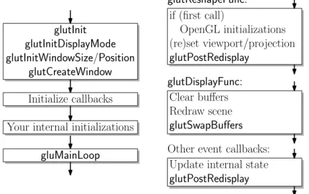
request to the system that the window be created. Why do you care? It is not possible to perform various graphics operations until notification has been received that the window is fully created. Your program is informed of this event through an event callback, eitherreshapeordisplay. We will discuss this below. The general structure of an OpenGL program using GLUT is shown in Fig. 6. Don’t worry if some elements are unfamiliar. We will discuss them below.

glutInit

glutInitDisplayMode

glutInitWindowSize/Position

glutCreateWindow

glutReshapeFunc:

Initialize callbacks

Your internal initializations

gluMainLoop

if (first call)

OpenGL initializations

(re)set viewport/projection

glutPostRedisplay

glutDisplayFunc:

Clear buffers

Redraw scene

glutSwapBuffers

Other event callbacks:

Update internal state

glutPostRedisplay

Event-driven Programming and Callbacks: Virtually all interactive graphics programs are event driven. Unlike traditional programs that read from a standard input file, a graphics program must be prepared at any time for input from any number of sources, including the mouse, or keyboard, or other graphics devises such as trackballs and joysticks.

In OpenGL this is done through the use of callbacks. The graphics program instructs the system to invoke a particular procedure whenever an event of interest occurs, say, the mouse button is clicked. The graphics program indicates its interest, orregisters, for various events. This involves telling the window system which event type you are interested in, and passing it the name of a procedure you have written to handle the event. Types of Callbacks: Callbacks are used for two purposes, user input eventsandsystem events. User input events

include things such as mouse clicks, the motion of the mouse (without clicking) also called passive motion, keyboard hits. Note that your program is only signaled about events that happen to your window. For example, entering text into another window’s dialogue box will not generate a keyboard event for your program.

There are a number of different events that are generated by the system. There is one such special event that every OpenGL program must handle, called adisplay event. A display event is invoked when the system senses that the contents of the window need to be redisplayed, either because:

• the graphics window has completed its initial creation,

• an obscuring window has moved away, thus revealing all or part of the graphics window, • the program explicitly requests redrawing, by callingglutPostRedisplay.

Recall from above that the commandglutCreateWindowdoes not actually create the window, but merely requests that creation be started. In order to inform your program that the creation has completed, the system generates a display event. This is how you know that you can now start drawing into the graphics window.

Another type of system event is a reshape event. This happens whenever the window’s size is altered. The callback provides information on the new size of the window. Recall that your initial call toglutInitWindowSize is only taken as a suggestion of the actual window size. When the system determines the actual size of your window, it generates such a callback to inform you of this size. Typically, the first two events that the system will generate for any newly created window are a reshape event (indicating the size of the new window) followed immediately by a display event (indicating that it is now safe to draw graphics in the window).

Often in an interactive graphics program, the user may not be providing any input at all, but it may still be necessary to update the image. For example, in a flight simulator the plane keeps moving forward, even without user input. To do this, the program goes to sleep and requests that it be awakened in order to draw the next image. There are two ways to do this, atimer eventand anidle event. An idle event is generated every time the system has nothing better to do. This may generate a huge number of events. A better approach is to request a timer event. In a timer event you request that your program go to sleep for some period of time and that it be “awakened” by an event some time later, say 1/30 of a second later. InglutTimerFuncthe first argument gives the sleep time as an integer in milliseconds and the last argument is an integer identifier, which is passed into the callback function. Various input and system events and their associated callback function prototypes are given in Table 2.

Input Event Callback request User callback function prototype (returnvoid) Mouse button glutMouseFunc myMouse(int b, int s, int x, int y)

Mouse motion glutPassiveMotionFunc myMotion(int x, int y)

Keyboard key glutKeyboardFunc myKeyboard(unsigned char c, int x, int y) System Event Callback request User callback function prototype (returnvoid) (Re)display glutDisplayFunc myDisplay()

(Re)size window glutReshapeFunc myReshape(int w, int h) Timer event glutTimerFunc myTimer(int id)

Idle event glutIdleFunc myIdle()

Table 2: Common callbacks and the associated registration functions.

For example, the following code fragment shows how to register for the following events: display events, re-shape events, mouse clicks, keyboard strikes, and timer events. The functions likemyDrawandmyReshapeare supplied by the user, and will be described later.

Most of these callback registrations simply pass the name of the desired user function to be called for the corresponding event. The one exception isglutTimeFuncwhose arguments are the number of milliseconds to wait (an unsigned int), the user’s callback function, and an integer identifier. The identifier is useful if there are multiple timer callbacks requested (for different times in the future), so the user can determine which one caused this particular event.

Callback Functions: What does a typical callback function do? This depends entirely on the application that you are designing. Some examples of general form of callback functions is shown below.

Typical Callback Setup int main(int argc, char** argv)

{ ...

glutDisplayFunc(myDraw); // set up the callbacks glutReshapeFunc(myReshape);

glutMouseFunc(myMouse); glutKeyboardFunc(myKeyboard);

glutTimerFunc(20, myTimeOut, 0); // (see below) ...

}

Examples of Callback Functions for System Events

void myDraw() { // called to display window

// ...insert your drawing code here ... }

void myReshape(int w, int h) { // called if reshaped

windowWidth = w; // save new window size

windowHeight = h;

// ...may need to update the projection ...

glutPostRedisplay(); // request window redisplay }

void myTimeOut(int id) { // called if timer event // ...advance the state of animation incrementally...

glutPostRedisplay(); // request redisplay

glutTimerFunc(20, myTimeOut, 0); // request next timer event }

Note that the timer callback and the reshape callback both invoke the functionglutPostRedisplay. This proce-dure informs OpenGL that the state of the scene has changed and should be redrawn (by calling your drawing procedure). This might be requested in other callbacks as well.

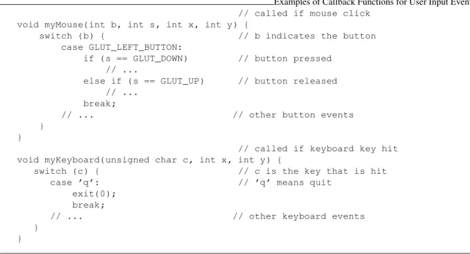
Examples of Callback Functions for User Input Events // called if mouse click

void myMouse(int b, int s, int x, int y) {

switch (b) { // b indicates the button

case GLUT_LEFT_BUTTON:

if (s == GLUT_DOWN) // button pressed // ...

else if (s == GLUT_UP) // button released // ...

break;

// ... // other button events

} }

// called if keyboard key hit void myKeyboard(unsigned char c, int x, int y) {

switch (c) { // c is the key that is hit

case ’q’: // ’q’ means quit

exit(0); break;

// ... // other keyboard events

} }

Note that each callback function is provided with information associated with the event. For example, a reshape event callback passes in the new window width and height. A mouse click callback passes in four arguments, which button was hit (b: left, middle, right), what the buttons new state is (s: up or down), the(x, y)coordinates of the mouse when it was clicked (in pixels). The various parameters used forbandsare described in Table 3.

A keyboard event callback passes in the character that was hit and the current coordinates of the mouse. The timer event callback passes in the integer identifier, of the timer event which caused the callback. Note that each call toglutTimerFunccreates only one request for a timer event. (That is, you do not get automatic repetition of timer events.) If you want to generate events on a regular basis, then insert a call toglutTimerFuncfrom within the callback function to generate the next one.

GLUT Parameter Name Meaning GLUT LEFT BUTTON left mouse button GLUT MIDDLE BUTTON middle mouse button GLUT RIGHT BUTTON right mouse button GLUT DOWN mouse button pressed down GLUT UP mouse button released

Table 3: GLUT parameter names associated with mouse events.

Basic Drawing: So far, we have shown how to create a window, how to get user input, but we have not discussed how to get graphics to appear in the window. Today we discuss OpenGL’s capabilities for drawing objects.

Before being able to draw a scene, OpenGL needs to know the following information: what are theobjectsto be drawn, how is the image to beprojectedonto the window, and howlightingandshadingare to be performed. To begin with, we will consider a very the simple case. There are only 2-dimensional objects, no lighting or shading. Also we will consider only relatively little user interaction.

Because we generally do not have complete control over the window size, it is a good idea to think in terms of drawing on a rectangularidealized drawing region, whose size and shape are completely under our control. Then we will scale this region to fit within the actual graphics window on the display. More generally, OpenGL allows for the grahics window to be broken up into smaller rectangular subwindows, calledviewports. We will then have OpenGL scale the image drawn in the idealized drawing region to fit within the viewport. The main advantage of this approach is that it is very easy to deal with changes in the window size.

We will consider a simple drawing routine for the picture shown in the figure. We assume that our idealized drawing region is a unit square over the real interval[0,1]×[0,1]. (Throughout the course we will use the

notation[a, b]to denote the interval of real valueszsuch thata≤z≤b. Hence,[0,1]×[0,1]is a unit square whose lower left corner is the origin.) This is illustrated in Fig. 7.

blue red 0 0.5 1 1 0.5 0

Fig. 7: Drawing produced by the simple display function.

Glut uses the convention that the origin is in the upper left corner and coordinates are given as integers. This makes sense for Glut, because its principal job is to communicate with the window system, and most window systems (X-windows, for example) use this convention. On the other hand, OpenGL uses the convention that coordinates are (generally) floating point values and the origin is in the lower left corner. Recalling the OpenGL goal is to provide us with an idealized drawing surface, this convention is mathematically more elegant. The Display Callback: Recall that thedisplay callback functionis the function that is called whenever it is necessary

to redraw the image, which arises for example:

• The initial creation of the window,

• Whenever the window is uncovered by the removal of some overlapping window,

• Whenever your program requests that it be redrawn (through the use ofglutPostRedisplay()function, as in

the case of an animation, where this would happen continuously.

The display callback function for our program is shown below. We first erase the contents of the image window, then do our drawing, and finally swap buffers so that what we have drawn becomes visible. (Recall double buffering from the previous lecture.) This function first draws a red diamond and then (on top of this) it draws a blue rectangle. Let us assume double buffering is being performed, and so the last thing to do is invoke glutSwapBuffers()to make everything visible.

Let us present the code, and we will discuss the various elements of the solution in greater detail below. Clearing the Window: The commandglClear()clears the window, by overwriting it with the background color. This

is set by the call

glClearColor(GLfloat Red, GLfloat Green, GLfloat Blue, GLfloat Alpha).

The type GLfloatis OpenGL’s redefinition of the standardfloat. To be correct, you should use the approved OpenGL types (e.g. GLfloat, GLdouble,GLint) rather than the obvious counterparts (float,double, and int). Typically the GL types are the same as the corresponding native types, but not always.

Sample Display Function

void myDisplay() // display function

{

glClear(GL_COLOR_BUFFER_BIT); // clear the window

glColor3f(1.0, 0.0, 0.0); // set color to red

glBegin(GL_POLYGON); // draw a diamond

glVertex2f(0.90, 0.50); glVertex2f(0.50, 0.90); glVertex2f(0.10, 0.50); glVertex2f(0.50, 0.10); glEnd();

glColor3f(0.0, 0.0, 1.0); // set color to blue

glRectf(0.25, 0.25, 0.75, 0.75); // draw a rectangle

glutSwapBuffers(); // swap buffers

}

Colors components are given as floats in the range from 0 to 1, from dark to light. Recall from Lecture 2 that theA(orα) value is used to control transparency. For opaque colorsAis set to 1. Thus to set the background

color to black, we would useglClearColor(0.0, 0.0, 0.0, 1.0), and to set it to blue useglClearColor(0.0, 0.0, 1.0, 1.0). (Hint: When debugging your program, it is often a good idea to use an uncommon background color, like a random shade of pink, since black can arise as the result of many different bugs.) Since the background color is usually independent of drawing, the functionglClearColor()is typically set in one of your initialization procedures, rather than in the drawing callback function.

Clearing the window involves resetting information within the frame buffer. As we mentioned before, the frame buffer may store different types of information. This includes color information, of course, but depth or distance information is used for hidden surface removal. Typically when the window is cleared, we want to clear everything, but occasionally it is possible to achieve special effects by erasing only part of the buffer (just the colors or just the depth values). So theglClear()command allows the user to select what is to be cleared. In this case we only have color in the depth buffer, which is selected by the optionGL COLOR BUFFER BIT. If we had a depth buffer to be cleared it as well we could do this by combining these using a “bitwise or” operation:

glClear(GL COLOR BUFFER BIT|GL DEPTH BUFFER BIT)

Drawing Attributes: The OpenGL drawing commands describe the geometry of the object that you want to draw. More specifically, all OpenGL is based on drawing objects with straight sides, so it suffices to specify the vertices of the object to be drawn. The manner in which the object is displayed is determined by various drawing attributes(color, point size, line width, etc.).

The command glColor3f()sets the drawing color. The arguments are three GLfloat’s, giving the R, G, and B components of the color. In this case, RGB = (1,0,0) means pure red. Once set, the attribute applies to all subsequently defined objects, until it is set to some other value. Thus, we could set the color, draw three polygons with the color, then change it, and draw five polygons with the new color.

This call illustrates a common feature of many OpenGL commands, namely flexibility in argument types. The suffix “3f” means that three floating point arguments (actuallyGLfloat’s) will be given. For example,glColor3d() takes three double(orGLdouble) arguments,glColor3ui() takes threeunsigned intarguments, and so on. For floats and doubles, the arguments range from 0 (no intensity) to 1 (full intensity). For integer types (byte, short, int, long) the input is assumed to be in the range from 0 (no intensity) to its maximum possible positive value (full intensity).

But that is not all! The three argument versions assume RGB color. If we were using RGBA color instead, we would useglColor4d()variant instead. Here “4” signifies four arguments. (Recall that the A or alpha value is used for various effects, such an transparency. For standard (opaque) color we setA= 1.0.)

In some cases it is more convenient to store your colors in an array with three elements. The suffix “v” means that the argument is a vector. For example glColor3dv()expects a single argument, a vector containing three GLdouble’s. (Note that this is a standard C/C++ style array, not the classvectorfrom the C++ Standard Template Library.) Using C’s convention that a vector is represented as a pointer to its first element, the corresponding argument type would be “const GLdouble*”.

Whenever you look up the prototypes for OpenGL commands, you often see a long list, some of which are shown below.

void glColor3d(GLdouble red, GLdouble green, GLdouble blue) void glColor3f(GLfloat red, GLfloat green, GLfloat blue) void glColor3i(GLint red, GLint green, GLint blue)

... (and forms for byte, short, unsigned byte and unsigned short) ... void glColor4d(GLdouble red, GLdouble green, GLdouble blue, GLdouble alpha) ... (and 4-argument forms for all the other types) ...

void glColor3dv(const GLdouble *v)

... (and other 3- and 4-argument forms for all the other types) ...

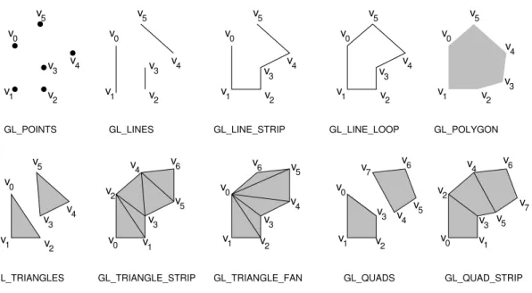
Drawing commands: OpenGL supports drawing of a number of different types of objects. The simplest isglRectf(), which draws a filled rectangle. All the others are complex objects consisting of a (generally) unpredictable number of elements. This is handled in OpenGL by the constructsglBegin(mode)andglEnd(). Between these two commands a list of vertices is given, which defines the object. The sort of object to be defined is determined by the modeargument of theglBegin()command. Some of the possible modes are illustrated in Fig. 8. For details on the semantics of the drawing methods, see the reference manuals.

Note that in the case ofGL POLYGONonlyconvex polygons(internal angles less than 180 degrees) are sup-ported. You must subdivide nonconvex polygons into convex pieces, and draw each convex piece separately.

glBegin(mode);

glVertex(v0); glVertex(v1); ... glEnd();

In the example above we only defined the x- and y-coordinates of the vertices. How does OpenGL know

whether our object is 2-dimensional or 3-dimensional? The answer is that it does not know. OpenGL represents all vertices as 3-dimensional coordinates internally. This may seem wasteful, but remember that OpenGL is designed primarily for 3-d graphics. If you do not specify thez-coordinate, then it simply sets thez-coordinate

to0.0. By the way,glRectf()always draws its rectangle on thez= 0plane.

Between any glBegin()...glEnd()pair, there is a restricted set of OpenGL commands that may be given. This includesglVertex()and also other command attribute commands, such asglColor3f(). At first it may seem a bit strange that you can assign different colors to the different vertices of an object, but this is a very useful feature. Depending on the shading model, it allows you to produce shapes whose color blends smoothly from one end to the other.

There are a number of drawing attributes other than color. For example, for points it is possible adjust their size (with glPointSize()). For lines, it is possible to adjust their width (withglLineWidth()), and create dashed or dotted lines (withglLineStipple()). It is also possible to pattern or stipple polygons (withglPolygonStipple()). When we discuss 3-dimensional graphics we will discuss many more properties that are used in shading and hidden surface removal.

v₅ v₄ v₂ v₁ v₀ v₃ GL_TRIANGLES v₀ v₁ v₂ v₄ v6 v₃ v₅ v₇ GL_QUAD_STRIP v₀ v_{1 v} 2 v_{3 v} 4 v₅ v₆ v₇ GL_QUADS v₃ v₀ v_{1 v} 2 v₄ v₅ v₆ GL_TRIANGLE_FAN v₃ v₀ v₁ v₂ v₅ v₄ v6 GL_TRIANGLE_STRIP v₅ v₄ v₂ v₁ v₀ v₃ GL_LINE_STRIP v₅ v₄ v₂ v₁ v₀ v₃ GL_LINE_LOOP v₅ v₂ v₁ v₀ v₄ v₃ GL_POLYGON v₅ v₄ v₃ v₂ v₁ v₀ GL_LINES v₅ v₄ v₃ v₂ v₁ v₀ GL_POINTS

Fig. 8: Some OpenGL object definition modes.

After drawing the diamond, we change the color to blue, and then invokeglRectf()to draw a rectangle. This procedure takes four arguments, the(x, y)coordinates of any two opposite corners of the rectangle, in this case (0.25,0.25)and(0.75,0.75). (There are also versions of this command that takes double or int arguments, and

vector arguments as well.) We could have drawn the rectangle by drawing aGL POLYGON, but this form is easier to use.

Viewports: OpenGL does not assume that you are mapping your graphics to the entire window. Often it is desirable to subdivide the graphics window into a set of smaller subwindows and then draw separate pictures in each window. The subwindow into which the current graphics are being drawn is called aviewport. The viewport is typically the entire display window, but it may generally be any rectangular subregion.

The size of the viewport depends on the dimensions of our window. Thus, every time the window is resized (and this includes when the window is created originally) we need to readjust the viewport to ensure proper transformation of the graphics. For example, in the typical case, where the graphics are drawn to the entire window, the reshape callback would contain the following call which resizes the viewport, whenever the window is resized.

Setting the Viewport in the Reshape Callback void myReshape(int winWidth, int winHeight) // reshape window

{ ...

glViewport (0, 0, winWidth, winHeight); // reset the viewport ...

}

The other thing that might typically go in themyReshape()function would be a call toglutPostRedisplay(), since you will need to redraw your image after the window changes size.

The general form of the command is

where(x, y)are the pixel coordinates of the lower-left corner of the viewport, as defined relative to the lower-left corner of the window, andwidthandheightare the width and height of the viewport in pixels.

Projection Transformation: In the simple drawing procedure, we said that we were assuming that the “idealized” drawing area was a unit square over the interval[0,1]with the origin in the lower left corner. The transformation that maps the idealized drawing region (in 2- or 3-dimensions) to the window is called theprojection. We did this for convenience, since otherwise we would need to explicitly scale all of our coordinates whenever the user changes the size of the graphics window.

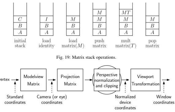
However, we need to inform OpenGL of where our “idealized” drawing area is so that OpenGL can map it to our viewport. This mapping is performed by a transformation matrix called theprojection matrix, which OpenGL maintains internally. (In future lectures, we will discuss OpenGL’s transformation mechanism in greater detail. In the mean time some of this may seem a bit arcane.)

Since matrices are often cumbersome to work with, OpenGL provides a number of relatively simple and natural ways of defining this matrix. For our 2-dimensional example, we will do this by simply informing OpenGL of the rectangular region of two dimensional space that makes up our idealized drawing region. This is handled by the command

gluOrtho2D(left, right, bottom, top).

First note that the prefix is “glu” and not “gl”, because this procedure is provided by the GLU library. Also, note that the “2D” designator in this case stands for “2-dimensional.” (In particular, it does not indicate the argument types, as with, say,glColor3f()).

All arguments are of type GLdouble. The arguments specify the x-coordinates (left andright) and the y

-coordinates (bottomandtop) of the rectangle into which we will be drawing. Any drawing that we do outside of this region will automatically be clipped away by OpenGL. The code to set the projection is given below.

Setting a Two-Dimensional Projection glMatrixMode(GL_PROJECTION); // set projection matrix

glLoadIdentity(); // initialize to identity

gluOrtho2D(0.0, 1.0, 0.0, 1.0); // map unit square to viewport

The first command tells OpenGL that we are modifying the projection transformation. (OpenGL maintains three different types of transformations, as we will see later.) Most of the commands that manipulate these matrices do so by multiplying some matrix times the current matrix. Thus, we initialize the current matrix to the identity, which is done byglLoadIdentity(). This code usually appears in some initialization procedure or possibly in the reshape callback.

Where does this code fragment go? It depends on whether the projection will change or not. If we make the simple assumption that are drawing will always be done relative to the [0,1]2_{unit square, then this code can} go in some initialization procedure. If our program decides to change the drawing area (for example, growing the drawing area when the window is increased in size) then we would need to repeat the call whenever the projection changes.

At first viewports and projections may seem confusing. Remember that the viewport is a rectangle within the actual graphics window on your display, where you graphics will appear. The projection defined bygluOrtho2D() simply defines a rectangle in some “ideal” coordinate system, which you will use to specify the coordinates of your objects. It is the job of OpenGL to map everything that is drawn in your ideal window to the actual viewport on your screen. This is illustrated in Fig. 9.

bottom top

right

Drawing gluOrtho2d glViewport

left

viewport

height

width (x,y)

idealized drawing region Your graphics window

Fig. 9: Projection and viewport transformations.

Lecture 4: Geometry and Geometric Programming

Geometric Programming: We are going to leave our discussion of OpenGL for a while, and discuss some of the basic elements of geometry, which will be needed for the rest of the course. There are many areas of computer science that involve computation with geometric entities. This includes not only computer graphics, but also areas like computer-aided design, robotics, computer vision, and geographic information systems. In this and the next few lectures we will consider how this can be done, and how to do this in a reasonably clean and painless way.

Computer graphics deals largely with the geometry of lines and linear objects in 3-space, because light travels in straight lines. For example, here are some typical geometric problems that arise in designing programs for computer graphics.

Geometric Intersections: Given a cube and a ray, does the ray strike the cube? If so which face? If the ray is reflected off of the face, what is the direction of the reflection ray?

Orientation: Three noncollinear points in 3-space define a unique plane. Given a fourth pointq, is it above,

below, or on this plane?

Transformation: Given unit cube, what are the coordinates of its vertices after rotating it 30 degrees about the vector(1,2,1).

Change of coordinates: A cube is represented relative to some standard coordinate system. What are its coor-dinates relative to a different coordinate system (say, one centered at the camera’s location)?

Such basic geometric problems are fundamental to computer graphics, and over the next few lectures, our goal will be to present the tools needed to answer these sorts of questions. (By the way, a good source of information on how to solve these problems is the series of books entitled “Graphics Gems”. Each book is a collection of many simple graphics problems and provides algorithms for solving them.)

There are various geometric systems. The principal ones that will be of interest to us are:

Affine Geometry: Geometric system involving “flat things”: points, lines, planes, line segments, triangles, etc. There is no defined notion of distance, angles, or orientations, however.

Euclidean Geometry: The geometric system that is most familiar to us. It enhances affine geometry by adding notions such as distances, angles, and orientations (such as clockwise and counterclockwise).

Projective Geometry: The geometric system needed for reasoning about perspective projection. Unfortu-nately, this system is not compatible with Euclidean geometry, as we shall see later.

#include <cstdlib> // standard definitions

#include <iostream> // C++ I/O

#include <GL/glut.h> // GLUT

#include <GL/glu.h> // GLU

#include <GL/gl.h> // OpenGL

using namespace std; // make std accessible

void myReshape(int w, int h) { // window is reshaped

glViewport (0, 0, w, h); // update the viewport

glMatrixMode(GL_PROJECTION); // update projection glLoadIdentity();

gluOrtho2D(0.0, 1.0, 0.0, 1.0); // map unit square to viewport glMatrixMode(GL_MODELVIEW);

glutPostRedisplay(); // request redisplay

}

void myDisplay(void) { // (re)display callback

glClearColor(0.5, 0.5, 0.5, 1.0); // background is gray glClear(GL_COLOR_BUFFER_BIT); // clear the window

glColor3f(1.0, 0.0, 0.0); // set color to red

glBegin(GL_POLYGON); // draw the diamond

glVertex2f(0.90, 0.50); glVertex2f(0.50, 0.90); glVertex2f(0.10, 0.50); glVertex2f(0.50, 0.10); glEnd();

glColor3f(0.0, 0.0, 1.0); // set color to blue

glRectf(0.25, 0.25, 0.75, 0.75); // draw the rectangle

glutSwapBuffers(); // swap buffers

}

int main(int argc, char** argv) {

glutInit(&argc, argv); // OpenGL initializations glutInitDisplayMode(GLUT_DOUBLE | GLUT_RGBA);// double buffering and RGB glutInitWindowSize(400, 400); // create a 400x400 window glutInitWindowPosition(0, 0); // ...in the upper left

glutCreateWindow(argv[0]); // create the window

glutDisplayFunc(myDisplay); // setup callbacks

glutReshapeFunc(myReshape);

glutMainLoop(); // start it running

return 0; // ANSI C expects this

}

You might wonder where linear algebra enters. We will make use of linear algebra as a concrete reprensenta-tional basis for these abstract geometric systems (in much the same way that a concrete structure like an array is used to represent an abstract structure like a stack in object-oriented programming). We will describe these systems, starting with the simplest, affine geometry.

Affine Geometry: The basic elements ofaffine geometryare:

• scalars, which we can just think of as being real numbers • points, which define locations in space

• free vectors (or simplyvectors), which are used to specify direction and magnitude, but have no fixed

position.

The term “free” means that vectors do not necessarily emanate from some position (like the origin), but float freely about in space. There is a special vector called the zero vector,~_{0, that has no magnitude, such that} ~v+~0 =~0 +~v=~v.

Note that we didnotdefine azero pointor “origin” for affine space. This is an intentional omission. No point special compared to any other point. (We will eventually have to break down and define an origin in order to have a coordinate system for our points, but this is a purely representational necessity, not an intrinsic feature of affine space.)

You might ask, why make a distinction between points and vectors? Both can be represented in the same way as a list of coordinates. The reason is to avoid hiding the intention of the programmer. For example, it makes perfect sense to multiply a vector and a scalar (we stretch the vector by this amount) or to add two vectors together (using the head-to-tail rule). It is not so clear what it means multiply a point by a scalar. (Such a point is twice as far away from the origin, but remember, there is no origin!) Similarly, what does it mean to add two points? Points are used for locations, vectors are used to denote direction and length. By keeping these basic concepts separate, the programmer’s intentions are easier to understand.

We will use the following notational conventions. Points will usually be denoted by lower-case Roman letters such asp,q, andr. Vectors will usually be denoted with lower-case Roman letters, such asu,v, andw, and

often to emphasize this we will add an arrow (e.g.,~u,~v,w~). Scalars will be represented as lower case Greek

letters (e.g.,α,β,γ). In our programs scalars will be translated to Roman (e.g.,a,b,c). (We will sometimes

violate these conventions, however. For example, we may use cto denote the center point of a circle orrto

denote the scalar radius of a circle.)

Affine Operations: The table below lists the valid combinations of these entities. The formal definitions are pretty much what you would expect. Vector operations are applied in the same way that you learned in linear algebra. For example, vectors are added in the usual “tail-to-head” manner (see Fig. 11). The differencep−qof two

points results in a free vector directed fromqtop. Point-vector additionr+~vis defined to be the translation

ofrby displacement~v. Note that some operations (e.g. scalar-point multiplication, and addition of points) are

explicitly not defined.

vector←scalar·vector, vector←vector/scalar scalar-vector multiplication

vector←vector+vector, vector←vector−vector vector-vector addition

vector←point−point point-point difference

point←point+vector, point←point−vector point-vector addition

Affine Combinations: Although the algebra of affine geometry has been careful to disallow point addition and scalar multiplication of points, there is a particular combination of two points that we will consider legal. The operation is called anaffine combination.

Let’s say that we have two pointspandqand want to compute their midpointr, or more generally a pointrthat

u

v

u

+

v

q

p

p

−

q

r

v

r

+

v

Vector addition

Point subtraction

Point-vector addition

case of the midpoint). This could be done by taking the vectorq−p, scaling it byα, and then adding the result

top. That is,

r=p+α(q−p).

Another way to think of this pointris as aweighted averageof the endpointspandq. Thinking ofrin these

terms, we might be tempted to rewrite the above formula in the following (illegal) manner:

r= (1−α)p+αq.

Observe that asαranges from 0 to 1, the pointrranges along the line segment fromptoq. In fact, we may

allow to become negative in which caserlies to the left ofp(see Fig. 12), and ifα >1, thenrlies to the right

ofq. The special case when0≤α≤1, this is called aconvex combination.

p

r

=

p

+

(

q

−

p

)

q

p

p

+

q

q

p

q

α <

0

0

< α <

1

α >

1

(1

−

α

)

p

+

αq

Fig. 12: Affine combinations.

In general, we define the following two operations for points in affine space.

Affine combination: Given a sequence of pointsp1, p2, . . . , pn, an affine combination is any sum of the form

α1p1+α2p2+. . .+αnpn, whereα1, α2, . . . , αnare scalars satisfyingP_iαi= 1.

Convex combination: Is an affine combination, where in addition we haveαi≥0for1≤i≤n.

Affine and convex combinations have a number of nice uses in graphics. For example, any three noncollinear points determine a plane. There is a 1–1 correspondence between the points on this plane and the affine combina-tions of these three points. Similarly, there is a 1–1 correspondence between the points in the triangle determined by the these points and the convex combinations of the points. In particular, the point(1/3)p+ (1/3)q+ (1/3)r

is thecentroidof the triangle.

We will sometimes be sloppy, and write expressions of the following sort (which is clearly illegal).

r= p+q 2 .

We will allow this sort of abuse of notation provided that it is clear that there is a legal affine combination that underlies this operation.

To see whether you understand the notation, consider the following questions. Given three points in the 3-space, what is the union of all their affine combinations? (Ans: the plane containing the 3 points.) What is the union of all their convex combinations? (Ans: The triangle defined by the three points and its interior.)

Euclidean Geometry: In affine geometry we have provided no way to talk about angles or distances. Euclidean geometry is an extension of affine geometry which includes one additional operation, called theinner product. The inner product is an operator that maps two vectors to a scalar. The product of~uand~vis denoted commonly

denoted(~u, ~v). There are many ways of defining the inner product, but any legal definition should satisfy the

following requirements

Positiveness: (~u, ~u)≥0and(~u, ~u) = 0if and only if~u=~0. Symmetry: (~u, ~v) = (~v, ~u).

Bilinearity: (~u, ~v+w~) = (~u, ~v) + (~u, ~w), and(~u, α~v) =α(~u, ~v). (Notice that the symmetric forms follow by

symmetry.)

See a book on linear algebra for more information. We will focus on a the most familiar inner product, called the dot product. To define this, we will need to get our hands dirty with coordinates. Suppose that thed-dimensional

vector~uis represented by the coordinate vector(u0, u1, . . . , ud−1). Then define

~u·~v= d−1 X i=0

uivi,

Note that inner (and hence dot) product is defined only for vectors, not for points.

Using the dot product we may define a number of concepts, which are not defined in regular affine geometry (see Fig. 13). Note that these concepts generalize to all dimensions.

Length: of a vector~vis defined to bek~vk=√~v·~v.

Normalization: Given any nonzero vector~v, define thenormalizationto be a vector of unit length that points

in the same direction as~v. We will denote this bybv:

b

v= ~v

k~vk.

Distance between points: dist(p, q) =kp−qk.

Angle: between two nonzero vectors~uand~v(ranging from 0 toπ) is

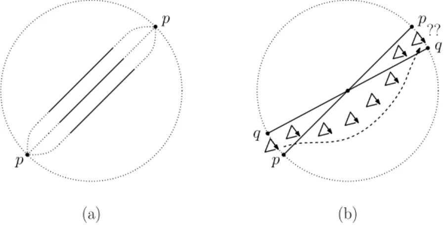
ang(~u, ~v) = cos−1

~u·~v

k~ukk~vk

= cos−1(bu·bv).

This is easy to derive from the law of cosines. Note that this does not provide us with a signed angle. We cannot tell whether~uis clockwise our counterclockwise relative to~v. We will discuss signed angles when

we consider the cross-product.

Orthogonality: ~uand~vareorthogonal(or perpendicular) if~u·~v= 0.

Orthogonal projection: Given a vector~uand a nonzero vector~v, it is often convenient to decompose~uinto

the sum of two vectors~u=~u1+~u2, such that~u1is parallel to~vand~u2is orthogonal to~v.

~u1 = (~u·~v)

(~v·~v)~v ~u2 = ~u−~u1.

(As an exercise, verify that~u2is orthogonal to~v.) Note that we can ignore the denominator if we know that~vis already normalized to unit length. The vector~u1is called theorthogonal projectionof~uonto~v.

v

θ

u

u

v

u

u

Angle between vectors

Orthogonal projection and its complement

Bases, Vectors, and Coordinates: Last time we presented the basic elements of affine and Euclidean geometry: p