7 Network Models. 7.1 Introduction

7

Network Models

7.1 Introduction

Extensive synaptic connectivity is a hallmark of neural circuitry. For ex-ample, a typical neuron in the mammalian neocortex receives thousands of synaptic inputs. Network models allow us to explore the computational potential of such connectivity, using both analysis and simulations. As illustrations, we study in this chapter how networks can perform the fol-lowing tasks: coordinate transformations needed in visually guided reach-ing, selective amplification leading to models of simple and complex cells in primary visual cortex, integration as a model of short-term memory, noise reduction, input selection, gain modulation, and associative mem-ory. Networks that undergo oscillations are also analyzed, with applica-tion to the olfactory bulb. Finally, we discuss network models based on stochastic rather than deterministic dynamics, using the Boltzmann ma-chine as an example.

Neocortical circuits are a major focus of our discussion. In the neocor-tex, which forms the convoluted outer surface of the (for example) human brain, neurons lie in six vertical layers highly coupled within cylindrical

columns. Such columns have been suggested as basic functional units, cortical columns and stereotypical patterns of connections both within a column and

be-tween columns are repeated across cortex. There are three main classes of interconnections within cortex, and in other areas of the brain as well.

Feedforward connections bring input to a given region from another re- feedforward, recurrent, and top-down connections gion located at an earlier stage along a particular processing pathway.

Re-current synapses interconnect neurons within a particular region that are considered to be at the same stage along the processing pathway. These may include connections within a cortical column as well as connections between both nearby and distant cortical columns within a region. Top-down connections carry signals back from areas located at later stages. These definitions depend on the how the region being studied is specified and on the hierarchical assignment of regions along a pathway. In gen-eral, neurons within a given region send top-down projections back to the areas from which they receive feedforward input, and receive top-down input from the areas to which they project feedforward output. The num-bers, though not necessarily the strengths, of feedforward and top-down

fibers between connected regions are typically comparable, and recurrent synapses typically outnumber feedforward or top-down inputs. We be-gin this chapter by studying networks with purely feedforward input and then study the effects of recurrent connections. The analysis of top-down connections, for which it is more difficult to establish clear computational roles, is left until chapter 10.

The most direct way to simulate neural networks is to use the methods dis-cussed in chapters 5 and 6 to synaptically connect model spiking neurons. This is a worthwhile and instructive enterprise, but it presents significant computational, calculational, and interpretational challenges. In this chap-ter, we follow a simpler approach and construct networks of neuron-like units with outputs consisting of firing rates rather than action potentials. Spiking models involve dynamics over time scales ranging from channel openings that can take less than a millisecond, to collective network pro-cesses that may be several orders of magnitude slower. Firing-rate models avoid the short time scale dynamics required to simulate action potentials and thus are much easier to simulate on computers. Firing-rate models also allow us to present analytic calculations of some aspects of network dynamics that could not be treated in the case of spiking neurons. Finally, spiking models tend to have more free parameters than firing-rate models, and setting these appropriately can be difficult.

There are two additional arguments in favor of firing-rate models. The first concerns the apparent stochasticity of spiking. The models discussed in chapters 5 and 6 produce spike sequences deterministically in response to injected current or synaptic input. Deterministic models can predict spike sequences accurately only if all their inputs are known. This is un-likely to be the case for the neurons in a complex network, and network models typically include only a subset of the many different inputs to indi-vidual neurons. Therefore, the greater apparent precision of spiking mod-els may not actually be realized in practice. If necessary, firing-rate modmod-els can be used to generate stochastic spike sequences from a deterministically computed rate, using the methods discussed in chapters 1 and 2.

The second argument involves a complication with spiking models that arises when they are used to construct simplified networks. Although cor-tical neurons receive many inputs, the probability of finding a synaptic connection between a randomly chosen pair of neurons is actually quite low. Capturing this feature, while retaining a high degree of connectiv-ity through polysynaptic pathways, requires including a large number of neurons in a network model. A standard way of dealing with this problem is to use a single model unit to represent the average response of several neurons that have similar selectivities. These “averaging” units can then be interconnected more densely than the individual neurons of the actual network, so fewer of them are needed to build the model. If neural re-sponses are characterized by firing rates, the output of the model unit is simply the average of the firing rates of the neurons it represents collec-tively. However, if the response is a spike, it is not clear how the spikes of the represented neurons can be averaged. The way spiking models are

7.2 Firing-Rate Models 231 typically constructed, an action potential fired by the model unit dupli-cates the effect of all the neurons it represents firing synchronously. Not surprisingly, such models tend to exhibit large-scale synchronization un-like anything seen in a healthy brain.

Firing-rate models also have their limitations. They cannot account for aspects of spike timing and spike correlations that may be important for understanding nervous system function. Firing-rate models are restricted to cases where the firing of neurons in a network is uncorrelated, with little synchronous firing, and where precise patterns of spike timing are unim-portant. In such cases, comparisons of spiking network models with mod-els that use firing-rate descriptions have shown that they produce similar results. Nevertheless, the exploration of neural networks undoubtedly re-quires the use of both firing-rate and spiking models.

7.2 Firing-Rate Models

As discussed in chapter 1, the sequence of spikes generated by a neuron is completely characterized by the neural response functionρ(t), which consists ofδfunction spikes located at times when the neuron fired action potentials. In firing-rate models, the exact description of a spike sequence provided by the neural response functionρ(t)is replaced by the approxi-mate description provided by the firing rater(t). Recall from chapter 1 that r(t)is defined as the probability density of firing and is obtained fromρ(t)

by averaging over trials. The validity of a firing-rate model depends on how well the trial-averaged firing rate of network units approximates the effect of actual spike sequences on the dynamic behavior of the network. The replacement of the neural response function by the corresponding fir-ing rate is typically justified by the fact that each network neuron has a large number of inputs. Replacingρ(t), which describes an actual spike train, with the trial-averaged firing rater(t)is justified if the quantities of relevance for network dynamics are relatively insensitive to the trial-to-trial fluctuations in the spike sequences represented byρ(t). In a network model, the relevant quantities that must be modeled accurately are the total inputs for the neurons within the network. For any single synaptic input, the trial-to-trial variability is likely to be large. However, if we sum the input over many synapses activated by uncorrelated presynaptic spike trains, the mean of the total input typically grows linearly with the number of synapses, while its standard deviation grows only as the square root of the number of synapses. Thus, for uncorrelated presynaptic spike trains, using presynaptic firing rates in place of the actual presynaptic spike trains may not significantly modify the dynamics of the network. Conversely, a firing-rate model will fail to describe a network adequately if the presy-naptic inputs to a substantial fraction of its neurons are correlated. This can occur, for example, if the presynaptic neurons fire synchronously. The synaptic input arising from a presynaptic spike train is effectively

fil-tered by the dynamics of the conductance changes that each presynaptic action potential evokes in the postsynaptic neuron (see chapter 5) and the dynamics of propagation of the current from the synapse to the soma. The temporal averaging provided by slow synaptic or membrane dynamics can reduce the effects of spike-train variability and help justify the approx-imation of using firing rates instead of presynaptic spike trains. Firing-rate models are more accurate if the network being modeled has a significant amount of synaptic transmission that is slow relative to typical presynap-tic interspike intervals.

The construction of a firing-rate model proceeds in two steps. First, we determine how the total synaptic input to a neuron depends on the fir-ing rates of its presynaptic afferents. This is where we use firfir-ing rates to approximate neural response functions. Second, we model how the firing rate of the postsynaptic neuron depends on its total synaptic input. Firing-rate response curves are typically measured by injecting current into the soma of a neuron. We therefore find it most convenient to define the total synaptic input as the total current delivered to the soma as a result of all the synaptic conductance changes resulting from presynaptic action po-tentials. We denote this total synaptic current by Is. We then determine

synaptic current Is

the postsynaptic firing rate from Is. In general, Is depends on the

spa-tially inhomogeneous membrane potential of the neuron, but we assume that, other than during action potentials or transient hyperpolarizations, the membrane potential remains close to, but slightly below, the thresh-old for action potential generation. An example of this type of behavior is seen in the upper panels of figure 7.2. Isis then approximately equal to

the synaptic current that would be measured from the soma in a voltage-clamp experiment, except for a reversal of sign. In the next section, we model how Isdepends on presynaptic firing rates.

In the network models we consider, both the output from, and the input to, a neuron are characterized by firing rates. To avoid a proliferation of sub- and superscripts on the quantityr(t), we use the letter u to denote a presynaptic firing rate, andvto denote a postsynaptic rate. Note thatvis input rate u

output ratev used here to denote a firing rate, not a membrane potential. In addition, we use these two letters to distinguish input and output firing rates in network models, a convention we retain through the remaining chapters. When we consider multiple input or output neurons, we use vectors u and v to represent their firing rates collectively, with the components of these

input rate vector u

output rate vector v vectors representing the firing rates of the individual input and output units.

The Total Synaptic Current

Consider a neuron receiving Nusynaptic inputs labeled by b=1,2, . . . ,Nu

(figure 7.1). The firing rate of input b is denoted by ub, and the input rates

are represented collectively by the Nu-component vector u. We model how

consid-7.2 Firing-Rate Models 233

output

v

u

w

Figure 7.1 Feedforward inputs to a single neuron. Input rates u drive a neuron at an output ratevthrough synaptic weights given by the vector w.

ering how it depends on presynaptic spikes. If an action potential arrives at input b at time 0, we write the synaptic current generated in the soma of the postsynaptic neuron at time t aswbKs(t), wherewbis the synaptic

weight and Ks(t) is called the synaptic kernel. Collectively, the

synap-tic weights are represented by a synapsynap-tic weight vector w, which has Nu synaptic weights w

componentswb. The amplitude and sign of the synaptic current generated

by input b are determined bywb. For excitatory synapses,wb>0, and for

inhibitory synapses,wb<0. In this formulation of the effect of presynaptic

spikes, the probability of transmitter release from a presynaptic terminal is absorbed into the synaptic weight factorwb, and we do not include

short-term plasticity in the model (although this can be done by makingwb a

dynamic variable).

The synaptic kernel, Ks(t)≥0, describes the time course of the synaptic synaptic

kernel Ks(t)

current in response to a presynaptic spike arriving at time t=0. This time course depends on the dynamics of the synaptic conductance activated by the presynaptic spike, and also on both the passive and the active prop-erties of the dendritic cables that carry the synaptic current to the soma. For example, long passive cables broaden the synaptic kernel and slow its rise from 0. Cable calculations or multi-compartment simulations, such as those discussed in chapter 6, can be used to compute Ks(t)for a specific

dendritic structure. To avoid ambiguity, we normalize Ks(t)by requiring

its integral over all positive times to be 1. At this point, for simplicity, we use the same function Ks(t)to describe all synapses.

Assuming that the effects of the spikes at a single synapse sum linearly, the total synaptic current at time t arising from a sequence of presynaptic spikes occurring at input b at times tiis given by

wb ti<t Ks(t−ti)=wb t −∞dτKs(t−τ)ρb(τ) . (7.1) In the second expression, we have used the neural response function,

ρb(τ)=iδ(τ−ti), to describe the sequence of spikes fired by

presy-naptic neuron b. The equality follows from integrating over the sum ofδ functions in the definition ofρb(τ). If there is no nonlinear interaction

be-tween different synaptic currents, the total synaptic current coming from all presynaptic inputs is obtained simply by summing,

Is= Nu b=1 wb t −∞dτKs(t−τ)ρb(τ) . (7.2)

As discussed previously, the critical step in the construction of a firing-rate model is the replacement of the neural response functionρb(τ)in

equa-tion 7.2 with the firing rate of neuron b, ub(τ), so that we write

Is= Nu b=1 wb t −∞dτKs(t−τ)ub(τ) . (7.3) The synaptic kernel most frequently used in firing-rate models is an expo-nential, Ks(t)=exp(−t/τs)/τs. With this kernel, we can describe Is by a

differential equation if we take the derivative of equation 7.3 with respect to t, τsdIs dt = −Is+ Nu b=1 wbub= −Is+w·u. (7.4)

In the second equality, we have expressed the sumwbubas the dot

prod-uct of the weight and input vectors, w·u. In this and the following

chap-dot product

ters, we primarily use the vector versions of equations such as 7.4, but when we first introduce an important new equation, we often write it in its subscripted form as well.

Recall that K describes the temporal evolution of the synaptic current due to both synaptic conductance and dendritic cable effects. For an electro-tonically compact dendritic structure,τswill be close to the time constant

that describes the decay of the synaptic conductance. For fast synaptic conductances such as those due to AMPA glutamate receptors, this may be as short as a few milliseconds. For a long, passive dendritic cable,τs

may be larger than this, but its measured value is typically quite small.

The Firing Rate

Equation 7.4 determines the synaptic current entering the soma of a post-synaptic neuron in terms of the firing rates of the prepost-synaptic neurons. To finish formulating a firing-rate model, we must determine the postsynap-tic firing rate from our knowledge of Is. For constant synaptic current,

the firing rate of the postsynaptic neuron can be expressed asv=F(Is),

where F is the steady-state firing rate as a function of somatic input cur-rent. F is also called an activation function. F is sometimes taken to be activation

function F(Is) a saturating function such as a sigmoid function. This is useful in cases

where the derivative of F is needed in the analysis of network dynamics. It is also bounded from above, which can be important in stabilizing a net-work against excessively high firing rates. More often, we use a threshold linear function F(Is)=[Is−γ]+, whereγis the threshold and the notation thresholdγ

[ ]+ denotes half-wave rectification, as in previous chapters. For conve-nience, we treat Is in this expression as if it were measured in units of a

firing rate (Hz), that is, as if Isis multiplied by a constant that converts its

units from nA to Hz. This makes the synaptic weights dimensionless. The thresholdγalso has units of Hz.

7.2 Firing-Rate Models 235 For time-independent inputs, the relationv=F(Is)is all we need to know

to complete the firing-rate model. The total steady-state synaptic current predicted by equation 7.4 for time-independent u is Is=w·u. This

gener-ates a steady-state output firing ratev=v∞given by

v∞=F(w·u) . (7.5)

The steady-state firing rate tells us how a neuron responds to constant cur-rent, but not to a current that changes with time. To model time-dependent inputs, we need to know the firing rate in response to a time-dependent synaptic current Is(t). The simplest assumption is that this is still given

by the activation function, sov=F(Is(t)) even when the total synaptic

current varies with time. This leads to a firing-rate model in which the

dynamics arises exclusively from equation 7.4, firing-rate model with current dynamics

τsdIs

dt = −Is+w·u with v=F(Is) . (7.6) An alternative formulation of a firing-rate model can be constructed by assuming that the firing rate does not follow changes in the total synaptic current instantaneously, as was assumed for the model of equation 7.6. Ac-tion potentials are generated by the synaptic current through its effect on the membrane potential of the neuron. Due to the membrane capacitance and resistance, the membrane potential is, roughly speaking, a low-pass filtered version of Is(see the Mathematical Appendix). For this reason, the

time-dependent firing rate is often modeled as a low-pass filtered version of the steady-state firing rate,

τrdv

dt = −v+F(Is(t)) . (7.7) The constantτr in this equation determines how rapidly the firing rate

approaches its steady-state value for constant Is, and how closely vcan

follow rapid fluctuations for a time-dependent Is(t). Equivalently, it

mea-sures the time scale over whichvaverages F(Is(t)). The low-pass filtering

effect of equation 7.7 is described in the Mathematical Appendix in the context of electrical circuit theory. The argument we have used to moti-vate equation 7.7 would suggest thatτrshould be approximately equal to

the membrane time constant of the neuron. However, this argument really applies to the membrane potential, not the firing rate, and the dynamics of the two are not the same. Some network models use a value ofτrthat

is considerably less than the membrane time constant. We re-examine this issue in the following section.

The second model that we have described involves the pair of equa-tions 7.4 and 7.7. If one of these equaequa-tions relaxes to its equilibrium point much more rapidly than the other, the pair can be reduced to a single equation. We discuss cases in which this occurs in the following section. For example, ifτrτs, we can make the approximation that equation 7.7

model that is defined by equation 7.6. If instead, τr τs, we can make

the approximation that equation 7.4 comes to equilibrium quickly com-pared with equation 7.7. Then we can make the replacement Is=w·u in

equation 7.7 and write firing-rate equation

τrdv

dt = −v+F(w·u) . (7.8) For most of this chapter, we analyze network models described by the firing-rate dynamics of equation 7.8, although occasionally we consider networks based on equation 7.6.

Firing-Rate Dynamics

The firing-rate models described by equations 7.6 and 7.8 differ in their assumptions about how firing rates respond to and track changes in the input current to a neuron. In one case (equation 7.6), it is assumed that firing rates follow time-varying input currents instantaneously, without attenuation or delay. In the other case (equation 7.8), the firing rate is a low-pass filtered version of the input current. To study the relationship between input current and firing rate, it is useful to examine the firing rate of a spiking model neuron in response to a time-varying injected current, I(t). The model used for this purpose in figure 7.2 is an integrate-and-fire neuron receiving balanced excitatory and inhibitory synaptic input along with a current injected into the soma that is the sum of constant and oscil-lating components. This model was discussed in chapter 5. The balanced synaptic input is used to represent background input not included in the computation of Is, and it acts as a source of noise. The noise prevents

effects, such as locking of the spiking to the oscillations of the injected cur-rent, that would invalidate a firing-rate description.

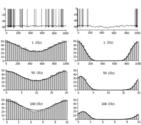
Figure 7.2 shows the firing rates of the model integrate-and-fire neuron in response to an input current I(t)= I0+I1cos(ωt). The firing rate is

plotted at different times during the cycle of the input current oscillations forω corresponding to frequencies of 1, 50, and 100 Hz. For the panels on the left side, the constant component of the injected current (I0) was

adjusted so the neuron never stopped firing during the cycle. In this case, the relationv(t)=F(I(t))(solid curves) provides an accurate description of the firing rate for all of the oscillation frequencies shown. As long as the neuron keeps firing fairly rapidly, the low-pass filtering properties of the membrane potential are not relevant for the dynamics of the firing rate. Low-pass filtering is irrelevant in this case, because the neuron is continually being shuttled between the threshold and reset values, so it never has a chance to settle exponentially anywhere near its steady-state value.

The right panels in figure 7.2 show that the situation is different if the input current is below the threshold for firing through a significant part

7.2 Firing-Rate Models 237 50 40 30 20 10 0 1000 800 600 400 200 0 50 40 30 20 10 0 20 15 10 5 0 10 8 6 4 2 0 time(ms) 1000 800 600 400 200 0 0 -60 -40 -20 1 (Hz) 50 (Hz) 100(Hz) 50 40 30 20 10 0 20 15 10 5 0 1000 800 600 400 200 0 10 8 6 4 2 0 1000 800 600 400 200 0 0 -60 -40 -20 time(ms) 50 40 30 20 10 0 50 40 30 20 10 0 50 40 30 20 10 0 1(Hz) 50(Hz) 100(Hz) firing rate (Hz) V (mV) firing rate (Hz) firing rate (Hz)

Figure 7.2 Firing rate of an integrate-and-fire neuron receiving balanced excitatory and inhibitory synaptic input and an injected current consisting of a constant and a sinusoidally varying term. For the left panels, the constant component of the in-jected current was adjusted so the firing never stopped during the oscillation of the varying part of the injected current. For the right panel, the constant component was lowered so the firing stopped during part of the cycle. The upper panels show two representative voltage traces of the model cell. The histograms beneath these traces were obtained by binning spikes generated over multiple cycles. They show the firing rate as a function of the time during each cycle of the injected current os-cillations. The different rows correspond to 1, 50, and 100 Hz oscillation frequen-cies for the injected current. The solid curves show the fit of a firing-rate model that involves both instantaneous and low-pass filtered effects of the injected cur-rent. For the left panel, this reduces to the simple predictionv=F(I(t)). (Adapted from Chance, 2000.)

of the oscillation cycle. In this case, the firing is delayed and attenuated at high frequencies, as would be predicted by equation 7.7. In this case, the membrane potential stays below threshold for long enough periods of time that its dynamics become relevant for the firing of the neuron. The essential message from figure 7.2 is that neither equation 7.6 nor equa-tion 7.8 provides a completely accurate predicequa-tion of the dynamics of the firing rate at all frequencies and for all levels of injected current. A more complex model can be constructed that accurately describes the firing rate over the entire range of input current amplitudes and frequencies. The solid curves in figure 7.2 were generated by a model that expresses the fir-ing rate as a function of both I from equation 7.6 andvfrom equation 7.8. In other words, it is a combination of the two models discussed in the

pre-output

v

W

u

B

A

M

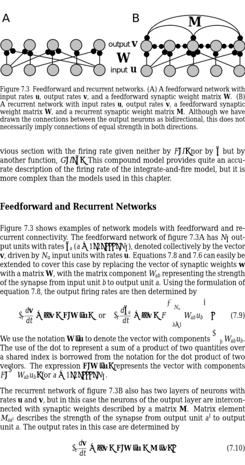
Figure 7.3 Feedforward and recurrent networks. (A) A feedforward network with input rates u, output rates v, and a feedforward synaptic weight matrix W. (B) A recurrent network with input rates u, output rates v, a feedforward synaptic weight matrix W, and a recurrent synaptic weight matrix M. Although we have drawn the connections between the output neurons as bidirectional, this does not necessarily imply connections of equal strength in both directions.

vious section with the firing rate given neither by F(I)nor by vbut by another function, G(I, v). This compound model provides quite an accu-rate description of the firing accu-rate of the integaccu-rate-and-fire model, but it is more complex than the models used in this chapter.

Feedforward and Recurrent Networks

Figure 7.3 shows examples of network models with feedforward and re-current connectivity. The feedforward network of figure 7.3A has Nv out-put units with ratesva(a=1,2, . . . ,Nv), denoted collectively by the vector v, driven by Nuinput units with rates u. Equations 7.8 and 7.6 can easily be

extended to cover this case by replacing the vector of synaptic weights w with a matrix W, with the matrix component Wabrepresenting the strength

of the synapse from input unit b to output unit a. Using the formulation of equation 7.8, the output firing rates are then determined by

feedforward model τrdv dt = −v+F(W·u) or τr dva dt = −v+F _Nu b=1 Wabub . (7.9) We use the notation W·u to denote the vector with components_bWabub.

The use of the dot to represent a sum of a product of two quantities over a shared index is borrowed from the notation for the dot product of two vectors. The expression F(W·u)represents the vector with components F(Wabub)for a=1,2, . . . ,Nv.

The recurrent network of figure 7.3B also has two layers of neurons with rates u and v, but in this case the neurons of the output layer are intercon-nected with synaptic weights described by a matrix M. Matrix element Maa describes the strength of the synapse from output unit a to output

unit a. The output rates in this case are determined by recurrent model

τrdv

7.2 Firing-Rate Models 239 It is often convenient to define the total feedforward input to each neuron in the network of figure 7.3B as h=W·u. Then, the output rates are determined by the equation

τrdv

dt = −v+F(h+M·v) . (7.11) Neurons are typically classified as either excitatory or inhibitory, meaning that they have either excitatory or inhibitory effects on all of their

postsy-naptic targets. This property is formalized in Dale’s law, which states that Dale’s law a neuron cannot excite some of its postsynaptic targets and inhibit others.

In terms of the elements of M, this means that for each presynaptic neuron a, Maa must have the same sign for all postsynaptic neurons a. To

im-pose this restriction, it is convenient to describe excitatory and inhibitory neurons separately. The firing-rate vectors vEand vIfor the excitatory and

inhibitory neurons are then described by a coupled set of equations

iden-tical in form to equation 7.11,

excitatory-inhibitory network τEdvE dt = −vE+FE(hE+MEE·vE+MEI·vI) (7.12) and τIdvI dt = −vI+FI(hI+MIE·vE+MII·vI) . (7.13) There are now four synaptic weight matrices describing the four possible types of neuronal interactions. The elements of MEE and MIE are greater

than or equal to 0, and those of MEI and MII are less than or equal to

0. These equations allow the excitatory and inhibitory neurons to have different time constants, activation functions, and feedforward inputs. In this chapter, we consider several recurrent network models described by equation 7.11 with a symmetric weight matrix, Maa=Maafor all a and

a. Requiring M to be symmetric simplifies the mathematical analysis, but symmetric coupling it violates Dale’s law. Suppose, for example, that neuron a, which is

exci-tatory, and neuron a, which is inhibitory, are mutually connected. Then, Maa should be negative and M_aapositive, so they cannot be equal.

Equa-tion 7.11 with symmetric M can be interpreted as a special case of equa-tions 7.12 and 7.13 in which the inhibitory dynamics are instantaneous (τI→0) and the inhibitory rates are given by vI=MIEvE. This produces

an effective recurrent weight matrix M=MEE+MEI·MIE, which can be

made symmetric by the appropriate choice of the dimension and form of the matrices MEI and MIE. The dynamic behavior of equation 7.11 is

re-stricted by requiring the matrix M to be symmetric. For example symmet-ric coupling typically does not allow for network oscillations. In the latter part of this chapter, we consider the richer dynamics of models described by equations 7.12 and 7.13.

Continuously Labeled Networks

It is often convenient to identify each neuron in a network by using a pa-rameter that describes some aspect of its selectivity rather than the integer label a or b. For example, neurons in primary visual cortex can be charac-terized by their preferred orientation angles, preferred spatial phases and frequencies, or other stimulus-related parameters (see chapter 2). In many of the examples in this chapter, we consider stimuli characterized by a single angle, which represents, for example, the orientation of a visual stimulus. Individual neurons are identified by their preferred stimulus angles, which are typically the values of for which they fire at maxi-mum rates. Thus, neuron a is identified by an angle θa. The weight of

the synapse from neuron b or neuron ato neuron a is then expressed as a function of the preferred stimulus anglesθb,θaandθaof the pre- and

post-synaptic neurons, Wab=W(θa, θb)or Maa=M(θa, θa). We often consider

cases in which these synaptic weight functions depend only on the differ-ence between the pre- and postsynaptic angles, so that Wab=W(θa−θb)

or Maa =M(θ_a−θ_a).

In large networks, the preferred stimulus parameters for different neurons will typically take a wide range of values. In the models we consider, the number of neurons is large and the angles θa, for different values of a,

cover the range from 0 to 2πdensely. For simplicity, we assume that this coverage is uniform, so that the density of coverage, the number of neu-rons with preferred angles falling within a unit range, which we denote byρθ, is constant. For mathematical convenience in these cases, we al-density of

coverageρθ low the preferred angles to take continuous values rather than restricting them to the actual discrete valuesθafor a=1,2, . . . ,N. Thus, we label

the neurons by a continuous angleθand express the firing rate as a func-tion of θ, so that u(θ)andv(θ)describe the firing rates of neurons with preferred anglesθ. Similarly, the synaptic weight matrices W and M are replaced by functions W(θ, θ)and M(θ, θ)that characterizes the strength of synapses from a presynaptic neuron with preferred angleθ_{to a} post-synaptic neuron with preferred angleθin the feedforward and recurrent cases, respectively.

If the number of neurons in a network is large and the density of cover-age of preferred stimulus values is high, we can approximate the sums in equation 7.10 by integrals over θ_{. The number of postsynaptic neurons} with preferred angles within a range θ_{isρθ θ, so, when we take the} limit θ_{→0, the integral overθ is multiplied by the density factorρθ.} Thus, in the case of continuous labeling of neurons, equation 7.10 becomes (for constantρθ) continuous model τrdv(θ) dt = −v(θ)+F ρθ _π −πdθ _{W(θ, θ)u(θ)+M(θ, θ)v(θ). (7.14)} As we did in equation 7.11, we can write the first term inside the integral of this expression as an input function h(θ). We make frequent use of continuous labeling for network models, and we often approximate sums over neurons by integrals over their preferred stimulus parameters.

7.3 Feedforward Networks 241

A

F

C

F

s

g

s+g

B

F

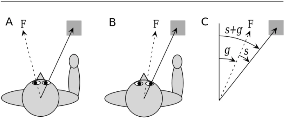
Figure 7.4 Coordinate transformations during a reaching task. (A, B) The location of the target (the gray square) relative to the body is the same in A and B, and thus the movements required to reach toward it are identical. However, the image of the object falls on different parts of the retina in A and B due to a shift in the gaze direction produced by an eye rotation that shifts the fixation point F. (C) The angles used in the analysis: s is the angle describing the location of the stimulus (the target) in retinal coordinates, that is, relative to a line directed to the fixation point; g is the gaze angle, indicating the direction of gaze relative to an axis straight out from the body. The direction of the target relative to the body is s+g.

7.3 Feedforward Networks

Substantial computations can be performed by feedforward networks in the absence of recurrent connections. Much of the work done on feed-forward networks centers on plasticity and learning, as discussed in the following chapters. Here, we present an example of the computational power of feedforward circuits, the calculation of the coordinate transfor-mations needed in visually guided reaching tasks.

Neural Coordinate Transformations

Reaching for a viewed object requires a number of coordinate transforma-tions that turn information about where the image of the object falls on the retina into movement commands in shoulder-, arm-, or hand-based coordinates. To perform a transformation from retinal to body-based co-ordinates, information about the retinal location of an image and about the direction of gaze relative to the body must be combined. Figure 7.4A and B illustrate, in a one-dimensional example, how a rotation of the eyes affects the relationship between gaze direction, retinal location, and loca-tion relative to the body. Figure 7.4C introduces the notaloca-tion we use. The angle g describes the orientation of a line extending from the head to the point of visual fixation. The visual stimulus in retinal coordinates is given by the angle s between this line and a line extending out to the target. The angle describing the reach direction, the direction to the target relative to the body, is the sum s+g.

Visual neurons have receptive fields fixed to specific locations on the retina. Neurons in motor areas can display visually evoked responses that

s (deg) s + g (deg) 0 60 20 40 80 100 -15 -30 0 15 30 45 60 A B s (deg) 20 -20 0 40 -40 C

firing rate (% max)

0 60 20 40 80 100 0 60 20 40 80 100 -15 -30 0 15 30 45 60 -45

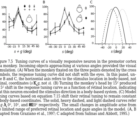
Figure 7.5 Tuning curves of a visually responsive neuron in the premotor cortex of a monkey. Incoming objects approaching at various angles provided the visual stimulation. (A) When the monkey fixated on the three points denoted by the cross symbols, the response tuning curve did not shift with the eyes. In this panel, un-like B and C, the horizontal axis refers to the stimulus location in body-based, not retinal, coordinates (s+g, not s). (B) Turning the monkey’s head by 15◦produced a 15◦shift in the response tuning curve as a function of retinal location, indicating that this neuron encoded the stimulus direction in a body-based system. (C) Model tuning curves based on equation 7.15 shift their retinal tuning to remain constant in body-based coordinates. The solid, heavy dashed, and light dashed curves refer to g=0◦, 10◦, and−20◦respectively. The small changes in amplitude arise from the limited range of preferred retinal location and gaze angles in the model. (A, B adapted from Graziano et al., 1997; C adapted from Salinas and Abbott, 1995.)

are not tied to specific retinal locations but, rather, depend on the relation-ship of a visual image to various parts of the body. Figures 7.5A and B show tuning curves of a neuron in the premotor cortex of a monkey that responded to visual images of approaching objects. Surprisingly, when the head of the monkey was held stationary during fixation on three different targets, the tuning curves did not shift as the eyes rotated (figure 7.5A). Although the recorded neurons respond to visual stimuli, the responses do not depend directly on the location of the image on the retina. When the head of the monkey is rotated but the fixation point remains the same, the tuning curves shift by precisely the amount of the head rotation (fig-ure 7.5B). Thus, these neurons encode the location of the image in a body-based, not a retinal, coordinate system.

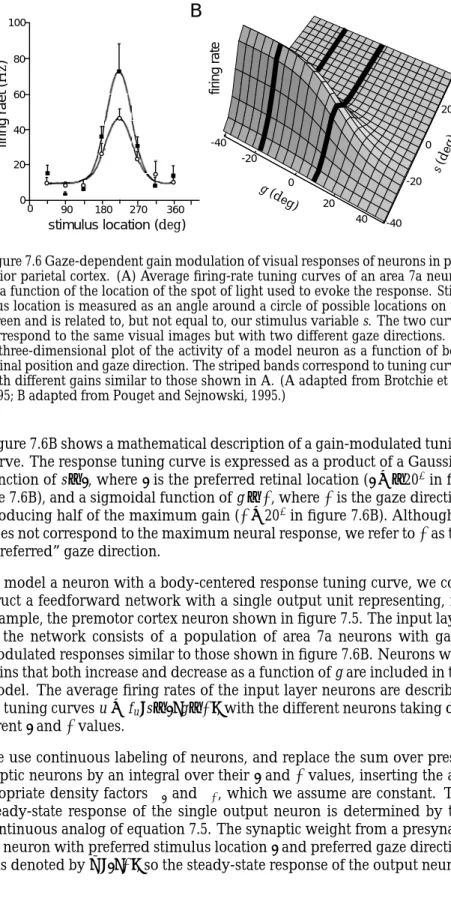
To account for these data, we need to construct a model neuron that is driven by visual input, but that nonetheless has a tuning curve for image location that is not a function of s, the retinal location of the image, but of s+g, the location of the object in body-based coordinates. A possible basis for this construction is provided by a combined representation of s and g by neurons in area 7a in the posterior parietal cortex of the monkey. Recordings made in area 7a reveal neurons that fire at rates that depend on both the location of the stimulating image on the retina and the direction of gaze (figure 7.6A). The response tuning curves, expressed as functions of the retinal location of the stimulus, do not shift when the direction of gaze is varied. Instead, shifts of gaze direction affect the magnitude of the visual response. Thus, responses in area 7a exhibit gaze-dependent gain modulation of a retinotopic visual receptive field.

7.3 Feedforward Networks 243 180 90 0 80 60 40 20 0 firing raet ( Hz )

A

stimulus location(deg)

100 --firing rate -40 -20 0 20 40 _-40 -20 0 20 40

B

Figure 7.6 Gaze-dependent gain modulation of visual responses of neurons in pos-terior parietal cortex. (A) Average firing-rate tuning curves of an area 7a neuron as a function of the location of the spot of light used to evoke the response. Stim-ulus location is measured as an angle around a circle of possible locations on the screen and is related to, but not equal to, our stimulus variable s. The two curves correspond to the same visual images but with two different gaze directions. (B) A three-dimensional plot of the activity of a model neuron as a function of both retinal position and gaze direction. The striped bands correspond to tuning curves with different gains similar to those shown in A. (A adapted from Brotchie et al., 1995; B adapted from Pouget and Sejnowski, 1995.)

Figure 7.6B shows a mathematical description of a gain-modulated tuning curve. The response tuning curve is expressed as a product of a Gaussian function of s−ξ, whereξis the preferred retinal location (ξ=−20◦in fig-ure 7.6B), and a sigmoidal function of g−γ, whereγis the gaze direction producing half of the maximum gain (γ=20◦ in figure 7.6B). Although it does not correspond to the maximum neural response, we refer toγas the “preferred” gaze direction.

To model a neuron with a body-centered response tuning curve, we con-struct a feedforward network with a single output unit representing, for example, the premotor cortex neuron shown in figure 7.5. The input layer of the network consists of a population of area 7a neurons with gain-modulated responses similar to those shown in figure 7.6B. Neurons with gains that both increase and decrease as a function of g are included in the model. The average firing rates of the input layer neurons are described by tuning curves u= fu(s−ξ,g−γ), with the different neurons taking

dif-ferentξandγvalues.

We use continuous labeling of neurons, and replace the sum over presy-naptic neurons by an integral over theirξandγvalues, inserting the ap-propriate density factorsρξ andργ, which we assume are constant. The steady-state response of the single output neuron is determined by the continuous analog of equation 7.5. The synaptic weight from a presynap-tic neuron with preferred stimulus locationξand preferred gaze direction

is given by v∞=F ρξργ dξdγ w(ξ, γ)fu(s−ξ,g−γ) . (7.15)

For the output neuron to respond to the stimulus location in body-based coordinates, its firing rate must be a function of s+g. To see if this is possible, we shift the integration variables in 7.15 byξ→ξ−g andγ→

γ+g. Ignoring effects from the end points of the integration (which is valid if s and g are not too close to these limits), we find

v∞=F ρξργ dξdγ w(ξ−g, γ+g)fu(s+g−ξ,−γ) . (7.16) This is a function of s+g provided thatw(ξ−g, γ+g)=w(ξ, γ), which holds ifw(ξ, γ)is a function of the sumξ+γ. Thus, the coordinate trans-formation can be accomplished if the synaptic weight from a given neuron depends only on the sum of its preferred retinal and gaze angles. It has been suggested that weights of this form can arise naturally from random hand and gaze movements through correlation-based synaptic modifica-tion of the type discussed in chapter 8.

Figure 7.5C shows responses predicted by equation 7.15 when the synaptic weights are given by a functionw(ξ+γ). The retinal location of the tuning curve shifts as a function of gaze direction, but would remain stationary if it were plotted instead as a function of s+g. This can be seen by noting that the peaks of all three curves in figure 7.5C occur at s+g=0.

Gain-modulated neurons provide a general basis for combining two dif-ferent input signals in a nonlinear way. In the network we studied, it is possible to find appropriate synaptic weightsw(ξ, γ) to generate output neuron responses with a wide range of different dependencies on s and g. The mechanism by which sensory and modulatory inputs combine in a multiplicative way in gain-modulated neurons is not known. Later in this chapter, we discuss a recurrent network model for generating gain-modulated responses.

7.4 Recurrent Networks

Recurrent networks have richer dynamics than feedforward networks, but they are more difficult to analyze. To get a feel for recurrent circuitry, we begin by analyzing a linear model, that is, a model for which the rela-tionship between firing rate and synaptic current is linear, F(h+M·v)= h+M·v. The linear approximation is a drastic one that allows, among other things, the components of v to become negative, which is impossi-ble for real firing rates. Furthermore, some of the features we discuss in connection with linear, as opposed to nonlinear, recurrent networks can also be achieved by a feedforward architecture. Nevertheless, the linear

7.4 Recurrent Networks 245 model is extremely useful for exploring properties of recurrent circuits, and this approach will be used both here and in the following chapters. In addition, the analysis of linear networks forms the basis for studying the stability properties of nonlinear networks. We augment the discussion of linear networks with results from simulations of nonlinear networks.

Linear Recurrent Networks

Under the linear approximation, the recurrent model of equation 7.11 takes

the form linear recurrent

model

τrdv

dt = −v+h+M·v. (7.17)

Because the model is linear, we can solve analytically for the vector of output rates v in terms of the feedforward inputs h and the initial values v(0). The analysis is simplest when the recurrent synaptic weight matrix is symmetric, and we assume this to be the case. Equation 7.17 can be solved by expressing v in terms of the eigenvectors of M. The eigenvectors eµfor

µ=1,2, . . . ,N_vsatisfy eigenvector e

M·e_µ=λµeµ (7.18)

for some value of the constantλµ, which is called the eigenvalue. For a eigenvalueλ symmetric matrix, the eigenvectors are orthogonal, and they can be

nor-malized to unit length so that eµ·eν =δµν. Such eigenvectors define an orthogonal coordinate system or basis that can be used to represent any

Nv-dimensional vector. In particular, we can write eigenvector expansion v(t)= Nv µ=1 cµ(t)eµ, (7.19)

where cµ(t)forµ=1,2, . . . ,Nv are a set of time-dependent coefficients describing v(t).

It is easier to solve equation 7.17 for the coefficients cµthan for v directly. Substituting the expansion 7.19 into equation 7.17 and using property 7.18, we find that τr Nv µ=1 dcµ dt eµ= − Nv µ=1 (1−λµ)cµ(t)eµ+h. (7.20) The sum overµcan be eliminated by taking the dot product of each side of this equation with one of the eigenvectors, eν, and using the orthogonality property eµ·eν=δµνto obtain

τrdcν

The critical feature of this equation is that it involves only one of the co-efficients, cν. For time-independent inputs h, the solution of equation 7.21 is cν(t)= ₁e₋ν·_λh ν 1−exp −t(1−λν) τr +cν(0)exp −t(1−λν) τr , (7.22) where cν(0)is the value of cνat time 0, which is given in terms of the initial firing-rate vector v(0)by cν(0)=eν·v(0).

Equation 7.22 has several important characteristics. Ifλν>1, the exponen-tial functions grow without bound as time increases, reflecting a funda-mental instability of the network. Ifλν<1, cνapproaches the steady-state value eν·h/(1−λν)exponentially with time constant τr/(1−λν). This steady-state value is proportional to eν·h, which is the projection of the input vector onto the relevant eigenvector. For 0< λν<1, the steady-state value is amplified relative to this projection by the factor 1/(1−λν), which is greater than 1. The approach to equilibrium is slowed relative to the ba-sic time constantτr by an identical factor. The steady-state value of v(t),

which we call v∞, can be derived from equation 7.19 as steady state v∞ v∞= Nv ν=1 (eν·h) 1−λνeν. (7.23)

This steady-state response can also arise from a purely feedforward scheme if the feedforward weight matrix is chosen appropriately, as we invite the reader to verify as an exercise.

Selective Amplification

Suppose that one of the eigenvalues of a recurrent weight matrix, denoted byλ1, is very close to 1, and all the others are significantly smaller than 1.

In this case, the denominator of theν=1 term on the right side of equa-tion 7.23 is near 0, and, unless e1·h is extremely small, this single term

will dominate the sum. As a result, we can write v∞≈ (e₁1₋·h_λ)e1

1 . (7.24)

Such a network performs selective amplification. The response is domi-nated by the projection of the input vector along the axis defined by e1,

and the amplitude of the response is amplified by the factor 1/(1−λ1),

which may be quite large ifλ1is near 1. The steady-state response of such

a network, which is proportional to e1, therefore encodes an amplified

pro-jection of the input vector onto e1.

Further information can be encoded if more eigenvalues are close to 1. Suppose, for example, that two eigenvectors, e1 and e2, have the same

7.4 Recurrent Networks 247 eigenvalue,λ1=λ2, close to but less than 1. Then, equation 7.24 is replaced

by

v∞≈ (e1·h)e₁1₋+_λ(e2·h)e2

1 , (7.25)

which shows that the network now amplifies and encodes the projection of the input vector onto the plane defined by e1and e2. In this case, the

ac-tivity pattern of the network is not simply scaled when the input changes. Instead, changes in the input shift both the magnitude and the pattern of network activity. Eigenvectors that share the same eigenvalue are termed degenerate, and degeneracy is often the result of a symmetry. Degener-acy is not limited to just two eigenvectors. A recurrent network with n degenerate eigenvalues near 1 can amplify and encode a projection of the input vector from the N-dimensional space in which it is defined onto the n-dimensional subspace spanned by the degenerate eigenvectors.

Input Integration

If the recurrent weight matrix has an eigenvalue exactly equal to 1,λ1=1,

and all the other eigenvalues satisfyλν<1, a linear recurrent network can act as an integrator of its input. In this case, c1satisfies the equation

τrdc1

dt =e1·h, (7.26)

obtained by settingλ1=1 in equation 7.21. For arbitrary time-dependent

inputs, the solution of this equation is c1(t)=c1(0)+ 1 τr

t 0

dte1·h(t) . (7.27)

If h(t)is constant, c1(t)grows linearly with t. This explains why

equa-tion 7.24 diverges asλ1→1. Suppose, instead, that h(t)is nonzero for a

while, and then is set to 0 for an extended period of time. When h=0, equation 7.22 shows that cν→0 for allν =1, because for these eigenvec-torsλν<1. Assuming that c1(0)=0, this means that after such a period,

the firing-rate vector is given, from equations 7.27 and 7.19, by network integration v(t)≈ e1 τr t 0 dte1·h(t) . (7.28)

This shows that the network activity provides a measure of the running integral of the projection of the input vector onto e1. One consequence of

this is that the activity of the network does not cease if h=0, provided that the integral up to that point in time is nonzero. The network thus exhibits sustained activity in the absence of input, which provides a memory of the integral of prior input.

Networks in the brain stem of vertebrates responsible for maintaining eye position appear to act as integrators, and networks similar to the one we

persistent activity eye position ON-direction burst neuron OFF-direction burst neuron integrator neuron

Figure 7.7 Cartoon of burst and integrator neurons involved in horizontal eye po-sitioning. The upper trace represents horizontal eye position during two saccadic eye movements. Motion of the eye is driven by burst neurons that move the eyes in opposite directions (second and third traces from top). The steady-state firing rate (labeled persistent activity) of the integrator neuron is proportional to the time integral of the burst rates, integrated positively for the ON-direction burst neuron and negatively for the OFF-direction burst neuron, and thus provides a memory trace of the maintained eye position. (Adapted from Seung et al., 2000.)

have been discussing have been suggested as models of this system. As outlined in figure 7.7, eye position changes in response to bursts of ac-tivity in ocular motor neurons located in the brain stem. Neurons in the medial vestibular nucleus and prepositus hypoglossi appear to integrate these motor signals to provide a persistent memory of eye position. The sustained firing rates of these neurons are approximately proportional to the angular orientation of the eyes in the horizontal direction, and activ-ity persists at an approximately constant rate when the eyes are held fixed (bottom trace in figure 7.7).

The ability of a linear recurrent network to integrate and display persis-tent activity relies on one of the eigenvalues of the recurrent weight matrix being exactly 1. Any deviation from this value will cause the persistent ac-tivity to change over time. Eye position does indeed drift, but matching the performance of the ocular positioning system requires fine-tuning of the eigenvalue to a value extremely close to 1. Including nonlinear inter-actions does not alleviate the need for a precisely tuned weight matrix. Synaptic modification rules can be used to establish the necessary synap-tic weights, but it is not clear how such precise tuning is accomplished in the biological system.

Continuous Linear Recurrent Networks

For a linear recurrent network with continuous labeling, the equation for the firing ratev(θ)of a neuron with preferred stimulus angleθis a linear version of equation 7.14, τrdv(θ) dt = −v(θ)+h(θ)+ρθ _π −πdθ _{M(θ−θ)v(θ) , (7.29)}

7.4 Recurrent Networks 249 where h(θ)is the feedforward input to a neuron with preferred stimulus angleθ, and we have assumed a constant densityρθ. Becauseθis an angle, h, M, andvmust all be periodic functions with period 2π. By making M a function ofθ−θ_{, we are imposing a symmetry with respect to translations} or shifts of the angle variables. In addition, we assume that M is an even function, M(θ−θ_{)= M(θ−θ). This is the analog, in a continuously} labeled model, of a symmetric synaptic weight matrix.

Equation 7.29 can be solved by methods similar to those used for discrete networks. We introduce eigenfunctions that satisfy

ρθ _π

−πdθ

_M(θ−θ)e

µ(θ)=λµeµ(θ) . (7.30) We leave it as an exercise to show that the eigenfunctions (normalized so thatρθtimes the integral from−πtoπof their square is 1) are 1/(2πρθ)1/2, corresponding to µ=0, and cos(µθ)/(πρθ)1/2 and sin(µθ)/(πρθ)1/2 for

µ=1,2, . . .. The eigenvalues are identical for the sine and cosine eigen-functions and are given (including the caseµ=0) by

λµ=ρθ _π

−πdθ

_{M(θ)cos(µθ) . (7.31)}

The steady-state firing rates for a constant input are given by the continu-ous analog of equation 7.23,

v∞(θ)= ₁₋1_λ 0 _π −π dθ 2π h(θ) +∞ µ=1 cos(µθ) 1−λµ _π −π dθ π h(θ)cos(µθ) +∞ µ=1 sin(µθ) 1−λµ π −π dθ π h(θ)sin(µθ) . (7.32)

The integrals in this expression are the coefficients in a Fourier series for Fourier series the function h and are known as cosine and sine Fourier integrals (see the

Mathematical Appendix).

Figure 7.8 shows an example of selective amplification by a linear recur-rent network. The input to the network, shown in panel A of figure 7.8, is a cosine function that peaks at 0◦to which random noise has been added. Figure 7.8C shows Fourier amplitudes for this input. The Fourier ampli-tude is the square root of the sum of the squares of the cosine and sine Fourier integrals. No particularµvalue is overwhelmingly dominant. In this and the following examples, the recurrent connections of the network are given by

M(θ−θ₎₌ λ1

πρθcos(θ−θ

_{) , (7.33)}

which has all eigenvalues exceptλ1equal to 0. The network model shown

-5 0 5 -180 -90 0 90 180 -20 -10 0 10 20 -180 -90 0 90 180 0 1 2 3 4 5 6 7 8 9 0 1 2 3 4 5 6 7 8 9 0 0.02 0.04 0.06 0.08 0.1 0 0.2 0.4 0.6 0.8 1

h

θ

θ

v

µ

µ

A

B

C

D

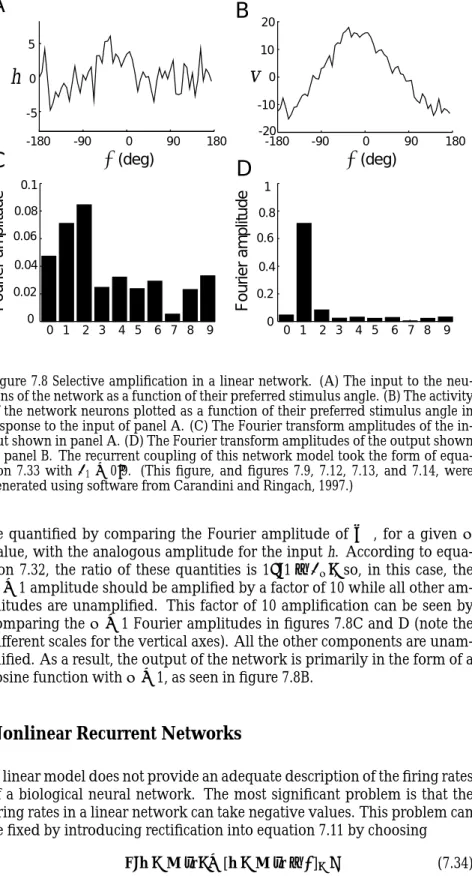
Figure 7.8 Selective amplification in a linear network. (A) The input to the neu-rons of the network as a function of their preferred stimulus angle. (B) The activity of the network neurons plotted as a function of their preferred stimulus angle in response to the input of panel A. (C) The Fourier transform amplitudes of the in-put shown in panel A. (D) The Fourier transform amplitudes of the outin-put shown in panel B. The recurrent coupling of this network model took the form of equa-tion 7.33 withλ1=0.9. (This figure, and figures 7.9, 7.12, 7.13, and 7.14, were

generated using software from Carandini and Ringach, 1997.)

be quantified by comparing the Fourier amplitude ofv∞, for a givenµ value, with the analogous amplitude for the input h. According to equa-tion 7.32, the ratio of these quantities is 1/(1−λµ), so, in this case, the

µ=1 amplitude should be amplified by a factor of 10 while all other am-plitudes are unamplified. This factor of 10 amplification can be seen by comparing theµ=1 Fourier amplitudes in figures 7.8C and D (note the different scales for the vertical axes). All the other components are unam-plified. As a result, the output of the network is primarily in the form of a cosine function withµ=1, as seen in figure 7.8B.

Nonlinear Recurrent Networks

A linear model does not provide an adequate description of the firing rates of a biological neural network. The most significant problem is that the firing rates in a linear network can take negative values. This problem can be fixed by introducing rectification into equation 7.11 by choosing rectification

7.4 Recurrent Networks 251 -5 0 -180 -90 0 90 180 0 20 40 60 80 -180 -90 0 90 180 0 1 2 3 4 5 6 7 8 9 0 0 1 2 3 4 5 6 7 8 9 0.2 0.4 0.6 0.8 1

θ

θ

v

(Hz)

µ

µ

A

B

C

D

Fourier amplitude Fourier amplitude

h

Figure 7.9 Selective amplification in a recurrent network with rectification. (A) The input h(θ)of the network plotted as a function of preferred angle. (B) The steady-state outputv(θ)as a function of preferred angle. (C) Fourier transform amplitudes of the input h(θ). (D) Fourier transform amplitudes of the outputv(θ). The recurrent coupling took the form of equation 7.33 withλ1=1.9.

whereγγγis a vector of threshold values that we often take to be 000 (we use the notation 000 to denote a vector with all its components equal to zero).

In this section, we show some examples illustrating the effect of including vector of zeros 000 such a rectifying nonlinearity. Some of the features of linear recurrent

net-works remain when rectification is included, but several new features also appear.

In the examples given below, we consider a continuous model, similar to that of equation 7.29, with recurrent couplings given by equation 7.33 but now including a rectification nonlinearity, so that

τrdv(θ) dt = −v(θ)+ h(θ)+λ1 π _π −πdθ _{cos(θ−θ)v(θ)} +. (7.35) Ifλ1is not too large, this network converges to a steady state for any

con-stant input (we consider conditions for steady-state convergence in a later section), and therefore we often limit the discussion to the steady-state ac-tivity of the network.

Nonlinear Amplification

Figure 7.9 shows the nonlinear analog of the selective amplification shown for a linear network in figure 7.8. Once again, a noisy input (figure 7.9A)

generates a much smoother output response profile (figure 7.9B). The out-put response of the rectified network corresponds roughly to the positive part of the sinusoidal response profile of the linear network (figure 7.8B). The negative output has been eliminated by the rectification. Because fewer neurons in the network have nonzero responses than in the linear case, the value of the parameterλ1in equation 7.33 has been increased to

1.9. This value, being larger than 1, would lead to an unstable network in the linear case. While nonlinear networks can also be unstable, the restric-tion to eigenvalues less than 1 is no longer the relevant condirestric-tion.

In a nonlinear network, the Fourier analysis of the input and output re-sponses is no longer as informative as it is for a linear network. Due to the rectification, theν=0,1, and 2 Fourier components are all amplified (figure 7.9D) compared to their input values (figure 7.9C). Nevertheless, except for rectification, the nonlinear recurrent network amplifies the in-put signal selectively in a manner similar to the linear network.

A Recurrent Model of Simple Cells in Primary Visual Cortex

In chapter 2, we discussed a feedforward model in which the elongated receptive fields of simple cells in primary visual cortex were formed by summing the inputs from neurons of the lateral geniculate nucleus (LGN) with their receptive fields arranged in alternating rows of ON and OFF cells. While this model quite successfully accounts for a number of fea-tures of simple cells, such as orientation tuning, it is difficult to reconcile with the anatomy and circuitry of the cerebral cortex. By far the majority of the synapses onto any cortical neuron arise from other cortical neurons, not from thalamic afferents. Therefore, feedforward models account for the response properties of cortical neurons while ignoring the inputs that are numerically most prominent. The large number of intracortical con-nections suggests, instead, that recurrent circuitry might play an impor-tant role in shaping the responses of neurons in primary visual cortex. Ben-Yishai, Bar-Or, and Sompolinsky (1995) developed a model in which orientation tuning is generated primarily by recurrent rather than feed-forward connections. The model is similar in structure to the model of equations 7.35 and 7.33, except that it includes a global inhibitory inter-action. In addition, because orientation angles are defined over the range from−π/2 toπ/2, rather than over the full 2πrange, the cosine functions in the model have extra factors of 2 in them. The basic equation of the model, as we implement it, is

τrdv(θ) dt = −v(θ)+ h(θ)+ _π/2 −π/2 dθ π −λ0+λ1cos(2(θ−θ)) v(θ₎ + , (7.36) wherev(θ)is the firing rate of a neuron with preferred orientationθ.

7.4 Recurrent Networks 253 The input to the model represents the orientation-tuned feedforward in-put arising from ON-center and OFF-center LGN cells responding to an oriented image. As a function of preferred orientation, the input for an image with orientation angle=0 is

h(θ)=Ac(1−+cos(2θ)) , (7.37) where A sets the overall amplitude and c is equal to the image contrast. The factor controls how strongly the input is modulated by the orien-tation angle. For=0, all neurons receive the same input, while=0.5 produces the maximum modulation consistent with a positive input. We study this model in the case whenis small, which means that the input is only weakly tuned for orientation and any strong orientation selectivity must arise through recurrent interactions.

To study orientation selectivity, we want to examine the tuning curves of individual neurons in response to stimuli with different orientation an-gles. The plots of network responses that we have been using show the firing rates v(θ)of all the neurons in the network as a function of their preferred stimulus angles θ when the input stimulus has a fixed value, typically=0. As a consequence of the translation invariance of the net-work model, the response for other values ofcan be obtained simply by shifting this curve so that it plotsv(θ−). Furthermore, except for the asymmetric effects of noise on the input,v(θ−)is a symmetric function. These features follow from the fact that the network we are studying is invariant with respect to translations and sign changes of the angle vari-ables that characterize the stimulus and response selectivities. An impor-tant consequence of this result is that the curvev(θ), showing the response of the entire population, can also be interpreted as the tuning curve of a single neuron. If the response of the population to a stimulus angleis

v(θ−), the response of a single neuron with preferred angle θ=0 is

v(−)=v()from the symmetry ofv. Becausev()is the tuning curve of a single neuron with θ=0 to a stimulus angle , the plots we show of v(θ)can be interpreted as both population responses and individual neuronal tuning curves.

Figure 7.10A shows the feedforward input to the model network for four different levels of contrast. Because the parameterwas chosen to be 0.1, the modulation of the input as a function of orientation angle is small. Due to network amplification, the response of the network is much more strongly tuned to orientation (figure 7.10B). This is the result of the selec-tive amplification of the tuned part of the input by the recurrent network. The modulation and overall height of the input curve in figure 7.10A in-crease linearly with contrast. The response shown in figure 7.10B, inter-preted as a tuning curve, increases in amplitude for higher contrast but does not broaden. This can be seen by noting that all four curves in fig-ure 7.10B go to 0 at the same two points. This effect, which occurs because the shape and width of the response tuning curve are determined primar-ily by the recurrent interactions within the network, is a feature of orien-tation curves of real simple cells, as seen in figure 7.10C. The width of the

firing rate ( Hz ) 80%_40% 20% 10% 80 60 40 20 0 180 200 220 240 (deg)

A

B

C

v

h

Figure 7.10 The effect of contrast on orientation tuning. (A) The feedforward in-put as a function of preferred orientation. The four curves, from top to bottom, correspond to contrasts of 80%, 40%, 20%, and 10%. (B) The output firing rates in response to different levels of contrast as a function of orientation preference. These are also the response tuning curves of a single neuron with preferred orien-tation 0. As in A, the four curves, from top to bottom, correspond to contrasts of 80%, 40%, 20%, and 10%. The recurrent model hadλ0=7.3,λ1=11, A=40 Hz,

and=0.1. (C) Tuning curves measured experimentally at four contrast levels, as indicated in the legend. (C adapted from Sompolinsky and Shapley, 1997 based on data from Sclar and Freeman, 1982.)

tuning curve can be reduced by including a positive threshold in the re-sponse function of equation 7.34, or by changing the amount of inhibition, but it stays roughly constant as a function of stimulus strength.

A Recurrent Model of Complex Cells in Primary Visual Cortex

In the model of orientation tuning discussed in the previous section, recur-rent amplification enhances selectivity. If the pattern of network connec-tivity amplifies nonselective rather than selective responses, recurrent in-teractions can also decrease selectivity. Recall from chapter 2 that neurons in the primary visual cortex are classified as simple or complex, depend-ing on their sensitivity to the spatial phase of a gratdepend-ing stimulus. Simple cells respond maximally when the spatial positioning of the light and dark regions of a grating matches the locations of the ON and OFF regions of their receptive fields. Complex cells do not have distinct ON and OFF re-gions in their receptive fields, and respond to gratings of the appropriate orientation and spatial frequency relatively independently of where their light and dark stripes fall. In other words, complex cells are insensitive to spatial phase.

Chance, Nelson, and Abbott (1999) showed that complex cell responses could be generated from simple cell responses by a recurrent network. As in chapter 2, we label spatial phase preferences by the angleφ. The feed-forward input h(φ)in the model is set equal to the rectified response of a simple cell with preferred spatial phaseφ (figure 7.11A). Each neuron in the network is labeled by the spatial phase preference of its