George Tzougas
Confidence intervals of the premiums of
optimal Bonus Malus Systems
Article (Accepted version)
(Refereed)
Original citation: Tzougas, George (2017) Confidence intervals of the premiums of optimal Bonus Malus Systems. Scandinavian Actuarial Journal . ISSN 0346-1238
DOI: 10.1080/03461238.2017.1307267
© 2017 Taylor & Francis
This version available at: http://eprints.lse.ac.uk/70926/
Available in LSE Research Online: May 2017
LSE has developed LSE Research Online so that users may access research output of the School. Copyright © and Moral Rights for the papers on this site are retained by the individual authors and/or other copyright owners. Users may download and/or print one copy of any article(s) in LSE Research Online to facilitate their private study or for non-commercial research. You may not engage in further distribution of the material or use it for any profit-making activities
or any commercial gain. You may freely distribute the URL (http://eprints.lse.ac.uk) of the LSE
Research Online website.
This document is the author’s final accepted version of the journal article. There may be differences between this version and the published version. You are advised to consult the publisher’s version if you wish to cite from it.
Confidence Intervals of the Premiums of
Optimal Bonus Malus Systems
Dimitris Karlis
∗Department of Statistics, Athens University of Economics and Business
Greece
George Tzougas
†Department of Statistics, London School of Economics, UK
Nicholas Frangos
Department of Statistics, Athens University of Economics and Business
Greece
Abstract
In view of the economic importance of motor third party liability insurance in developed countries the construction of optimal BMS has been given con-siderable interest. However, a major drawback in the construction of optimal BMS is that they fail to account for the variability on premium calculations which are treated as point estimates. The present study addresses this issue. Specifically, nonparametric mixtures of Poisson laws are used to construct an optimal BMS with a finite number of classes. The mixing distribution is estimated by nonparametric maximum likelihood (NPML). The main contri-bution of this paper is the use of the NPML estimator for the construction of confidence intervals for the premium rates derived by updating the posterior mean claim frequency. Furthermore, we advance one step further by improv-ing the performance of the confidence intervals based on a bootstrap proce-dure where the estimated mixture is used for resampling. The construction ∗Athens University of Economics and Business, 76 Patission Str., 104 34, Athens, Greece, Tel: +30 210 8203 920; fax: +30 210 8203 920. E-mail address: [email protected] (D. Karlis)
†Part of the work was done while Dr Tzougas was a postdoctoral researcher at Department of Statistics, Athens University of Economics and Business
of confidence intervals for the individual premiums based on the asymptotic maximum likelihood theory is beneficial for the insurance company as it can result in accurate and effective adjustments to the premium rating policies from a practical point of view.
Keywords: Optimal BMS; Nonparametric maximum likelihood; Asymptotic Normality; Wald type two-sided confidence intervals; Efron percentile boot-strap confidence intervals
1
Introduction
Bonus-Malus Systems, BMS in short, are experience rating mechanisms which im-pose penalties on policyholders responsible for one or more accidents by premium surcharges (or maluses) and reward discounts (or bonuses) to policyholders who had a claim-free year. Optimal BMS are financially balanced for the insurer, i.e. the total amount of bonuses must be equal to the total amount of maluses, and fair for the policyholder, i.e. the premium paid for each policyholder is proportional to the risk that they impose on the pool. The design of such systems is achieved through Bayesian analysis and the form of the mixed Poisson distributions which capture the unobserved heterogeneity of claim count data with respect to the simplistic Poisson law. Over the years numerous articles have been devoted to this topic as this is an area of applied statistics that has close ties with theoretical statistics, no-tably Bayesian Analysis, nonparametric maximum likelihood estimation, advanced regression models and credibility theory, which is the cornerstone of contemporary insurance mathematics. An excellent account of BMS can be found in Lemaire (1995). Also, references for BMS include, among others, Dionne and Vanasse (1989, 1992), Coene and Doray (1996), Walhin and Paris (1999), Pinquet (1998), Pinquet et al. (2001), Denuit and Lambert (2001), Brouhns et al. (2003), Denuit et al. (2007), Pitrebois et al. (2005), Boucher et al. (2008), Tzougas and Frangos (2014) and Tzougas et al. (2014).
However, even though the construction of optimal BMS has been a basic interest of actuarial literature for over four decades, scientific attention has only now focused on deriving credibility updates of the claim frequency based on the employment of an abundance of alternative parametric distributions, nonparametric distributions and advanced regression models. In this respect, a major drawback in the design
of such systems was neglected: namely the fact that they do not give a measure of uncertainty of the resulting premium estimates by providing a confidence interval that contains plausible values.
In a competitive insurance market, in order to avoid lapses, actuaries do not only have to construct optimal BMS that will fairly distribute the burden of claims among policyholders, as was the usual practice, but their designs also have to be able to adjust the individual premiums from a practical point of view . Moreover, taking into account that according to a 2015 report by Insurance Europe (Insurance Europe, 2015), an insurance and reinsurance federation with 34 member bodies, the largest non-life insurance market, motor insurance totaled 130.8bn Euros in premiums (stable in 2014), it becomes clear that the problem briefly described above can result in great losses for insurance companies operating in Europe.
Let us now explain how the present study addresses the aforementioned problem. In most settings involving count data, one of the biggest challenges that a researcher can come across is reliably estimating or building confidence intervals, CIs, for small and tail probabilities. In the majority of cases the available data are either insuffi-cient to allow for asymptotic arguments or they need to be smoothed to render them useful. In motor third party liability (MTPL) insurance, the interest of actuaries lies in identifying customers with high claim frequency but they normally represent very few observations. A simple and intuitive approach could be to resort to the use of the empirical proportion as an estimate of the event probability. However, a serious drawback of this method is the heavy data requirement. That is, if the event is not observed with sufficient frequency, tail probabilities cannot be estimated with accuracy. Therefore, smoother estimates for tail probabilities are demanded in order to produce useful results. As a solution to the aforementioned problem, one could consider a model where the small probabilities are connected to other parts of the probability distribution. However, in this case inference is vulnerable to model assumptions.
Karlis and Patilea (2008) proposed a satisfactory trade-off between the flexibil-ity of that model which guards against misspecification and the abilflexibil-ity to provide non-degenerated estimates with finite samples. Specifically, following B¨ohning and Patilea (2005), these authors considered nonparametric mixtures of power series dis-tributions and built CIs for small probabilities with count data based on the use of the nonparametric maximum likelihood estimator, NPMLE, of the mixing distribu-tion. Also, they constructed bootstrap two-sided confidence intervals based on a bootstrap from the NPMLE of the mixture. Furthermore, Karlis and Patilea (2007) constructed NPMLE and bootstrap based CIs for the hazard rate function of the
discrete lifetime distribution.
In this paper we extend BMS literature research by addressing the problem of building confidence intervals for the premiums determined by an optimal BMS in the following ways.
• Firstly, following Walhin and Paris (1999) and Denuit and Lambert (2001), we consider a flexible class of nonparametric mixtures of Poisson distributions for assessing claim frequency. An algorithm which is a variant of the EM algorithm adjusted for jumping between different numbers of components is proposed in order to estimate the unknown mixing, or risk, distribution based on nonparametric maximum likelihood estimation. The use of the nonpara-metric estimate of the risk distribution allows for a rich family of claim fre-quency distributions instead of restricting attention to particular laws such as the negative binomial distribution that has been widely applied for modelling claim count data. On the path toward actuarial relevance the Bayesian view is taken and the NPMLE of the risk distribution is used to calculate premi-ums as posterior means. Following Lambert and Tierney (1984) and B¨ohning and Patilea (2005), it is shown that the NPMLE based posterior mean claim frequency behaves asymptotically normal. Based on the asymptotic normality of the posterior mean claim frequency Wald type two-sided confidence inter-vals are constructed. The Wald CIs are not degenerated and therefore are more useful than the corresponding intervals based on model analogy or ad hoc reasoning.
• Secondly, we develop bootstrap two-sided confidence intervals for the individ-ual premiums based on bootstrap from the NPMLE of the mixing distribution. This NPMLE based resampling procedure is a common method encountered in the literature, see for example Laird and Louis (1987) and B¨ohning (2000). Refer also to Karlis and Patilea (2008) for the proof of its asymptotic validity. Specifically, Efron percentile bootstrap confidence intervals are investigated and compared to the Wald Type confidence intervals obtained directly from the NPML estimates. Our analysis reveals that Efron percentile bootstrap intervals on certain occasions improve the asymptotic normal approximation used by Wald intervals. The aforementioned constructions of NPMLE and bootstrap based CIs account for the uncertainty as well as the fluctuations of the individual premium estimates.
In an experience ratemaking scheme the use of such intervals leaves room for the informed judgment of the actuary to select the final premiums to be charged to
each policyholder based on the fluctuations that occur equally on either side of the credibility updates of their claim frequency. In this respect, the insurance company can be responsive to the needs of different constituencies, such as broader economic trends for the insurance market in which it operates or mounting regulatory require-ments, in order to make more accurate and effective adjustments to the tariff from a practical point of view.
The rest of the paper is as follows. Section 2 presents the general background on mixtures of Poisson distributions. Section 3 provides the computational details for the algorithm used for the NPMLE. Section 4 describes the design of an optimal BMS with a finite number of classes based on the NPMLE of the risk distribution. Section 5 provides the main results for the NPMLE based intervals and the bootstrap intervals respectively. Section 6 contains an application to a data set concerning car-insurance claims at fault. Finally, Section 7 presents the concluding remarks of the paper.
2
Mixtures of Poisson Distributions
Let us consider a Poisson mixture with probability mass function (pmf) given by
P(x;FΛ) =πFΛ(k) = Z
Λ
P(x;λ)FΛ(dλ), (1)
for k ∈ N, where P(x;λ) is the probability distribution function of the Poisson distribution and whereFΛ is the mixing distribution, that is a probability measure
on Λ, whose support isR+. Assume that the independent observations distributed according to the mixtureπFΛ0 with individual probabilitiesπFΛ0(k), k ∈N. The true
mixing distributionFΛ0 is unknown but its support is included in a known compact
interval [0, M] ⊂R+. In practice one can choose M to arbitrarily large. It is quite
typical to assume a certain parametric form for FΛ0(·) and fit a parametric model.
However, to gain more flexibility we prefer not to assume any parametric form for the mixing distribution and leave FΛ0 to be a general mixing distribution. There
are a wide range of practical applications for this type of model, as for example, population heterogeneity studies, non-parametric empirical Bayes estimation and semiparametric density estimation; see Lindsay (1995), Lindsay and Lesperance (1995), B¨ohning (2000) and the references therein.
By definition, FΛ0 is identifiable if FΛ0 = FΛ implies that Λ0 = Λ.
P
k>0,k∈Nk
−1 =∞holds, F
Λ0 is identifiable among all the mixing distributions with
the support in Λ.
In this study, we estimateFΛ0 in a nonparametric way and then use the Poisson
mixture for constructing an optimal BMS. Let X1, . . . , Xn ∈ N be an i.i.d. sample
with distribution πFΛ0. The log-likelihood function (denoted as a function of the
mixing distribution) is `(FΛ) = n X i=1 log Z Λ P(xi;λ)dFΛ(λ) . (2)
We want to maximize `(·) with respect to all distribution functions defined on Λ, this is called the nonparametric maximum likelihood estimator (NPMLE) and it is known to be a distribution with discrete support, i.e. giving positive probability to a finite number of points.
Hereafter, let ˆFΛ be the NPMLE of FΛ0.There are results on the maximum
number of support points ˆq (see Simar, 1976 and Lindsay, 1983), which cannot exceed the number of distinct values in the sample. Specifically, Simar (1976) was the first to show that the NPMLE will be unique under the following condition
ˆ q ≤min kmax+ 1 2 , κ ,
wherekmax is the maximum number of claims per risk andκis the number of classes
for with non-zero frequency. Furthermore, existence, support size, and other finite sample properties of ˆFΛ can be found in Simar (1976) and Lindsay (1995).
Concern-ing consistency, with probability one ˆFΛ →FΛ0 weakly, since FΛ0 is identifiable (see
for instance, van de Geer, 1993, Lemma 5.2). Furthermore, existence, support size, and other finite sample properties of ˆFΛ can be found in Simar (1976) and Lindsay
(1995). Since the NPMLE ˆFΛ is discrete the model resembles the finite mixture
model.
Methods like the widely used EM algorithm could be used towards the deriva-tion the NPMLE. Lambert and Tierney (1984) showed the asymptotic normality of the NPMLE for Poisson mixtures while B¨ohning and Patilea (2005) showed the asymptotic normality of the NPMLE for mixture of power series family (and hence for the Poisson case since it is a member of the power series family of distributions). Karlis and Patilea (2007, 2008) showed the consistency in probability of bootstrap confidence intervals and they applied this to the case of hazard function which is related to what follows here, since it involves ratio of probabilities as we will do for
the BMS case. Being able to derive such confidence intervals for the BMS we are able to account for the uncertainty around the premium calculated.
3
Computational Details
In this section we describe the algorithm used to derive the NPMLE. Algorithms for finding the NPMLE has been proposed by Laird (1978), Dersimonian (1986), Lesperance and Kalbfleisch (1992)(see also the book of B¨ohning (2000) for a broad review on these algorithms). Recent work can be found in Wang (2007). They make use of the gradient function in order to decide where to add new supports points and which one can be removed. The gradient function is defined as
d(λ;FΛ) = n X i=1 P(xi;λ) P(xi;FΛ) −n (3)
For the NPMLE it holds that supλd(λ,FˆΛ) = 0 (see Lindsay, 1995) and this
pro-vides a diagnostic whether the NPMLE has been found. Alternatively one may use algorithms for fixed number of support points k for different values of k. These algorithms are feasible for count data because the number of support points in the NPMLE is usually small (see the results of Lindsay, 1995).
The algorithm used in the present paper for finding the NPMLE is a variant of the EM algorithm adjusted for jumping between different numbers of components. Namely the algorithm starts with the maximum possible number of components (see Simar, 1976 and Lindsay, 1983). Then we keep iterating using the EM algorithm until either satisfaction of the convergence criterion (measured by the change of the relative likelihood) or until a redundant support points is found. A support point is redundant either if a) two points are close together or b) one mixing proportion is close to 0. Two components with parameters, say λj and λk are considered as
being close together if |λj − λk| < 10−6. If this is the case, then, we check if
combining these components in a single component with value the weighted average of the two components and mixing proportion the sum of the two proportions, we can improve the likelihood. If the likelihood can be improved, the components are merged, otherwise we keep iterating retaining both the components. The idea for this step is that if the components are close together then this implies either that the components must be merged or that the likelihood will remain trapped in this area for a long time. If the second is true our algorithm can fail, but in any case we will not waste our time waiting to pass over the flat point. Note that our experience
was that typically two point so close should be merged. A mixing proportion is close to 0 if its value is smaller than a threshold like 10−6. In the case of a small mixing
proportions we just remove this point by rescaling the other mixing proportions to sum to 1. Note that, very small mixing proportions are expected only for large sample sizes.
When the algorithm converges (i.e. the relative change of the log-likelihood is smaller than 10−12, we check whether the NPMLE has been found by using the
conditions given in Lindsay (1995). These conditions were based on the gradient function defined in (3). We calculated the gradient function over a grid of 1000 points in a large interval from 0 to 1.2λmax, where λmax is she largest support point
and we checked whether for all the points the gradient was less than 0.0001. If the solution was not truly a NPMLE (i.e. the function lies above zero) then we rerun the EM algorithm described above from different initial values.
For every repetition, initial values were chosen randomly over the interval of admissible values. For each sample 20 different initial values were considered. If the NPMLE was not found after 20 runs then we rejected this sample. The rate of rejecting samples was smaller than 2% for the Poisson case. Note also that, since we are not interested about reporting the number of support points, redundant points in the NPMLE do not cause any problem since the probabilities estimated by the NPMLE will coincide. Our algorithm is similar to running an EM with fixed support size equal to the maximum possible for each sample. Our algorithm improved on this approach by reducing the dimensionality between iterations and thus removing redundant calculations at each iteration.
A step by step description of the algorithm follows. Technical details are not repeated.
Step 0: Start with k support points. Choose initial values for the parameters.
Step 1: Run a number of EM iterations, say M (M can be one but usually a larger value improves speed)
Step 2: Check if there are redundant support points: i.e. points, withλ close together or mixing proportion close to 0.
Step 3a: If redundant points are found then merge them (or discard the one with a almost zero mixing proportion).
Step 3b: If the loglikelihood after merging is improved then keep going with the merged components and go back to Step 1, else keep going with the same number of
components.
Step 4: Check if convergence is detected and stop otherwise go back to Step 1. Step 5: Use the gradient function to ensure that the NPMLE is found. If not use other
initial values and go back to Step 0.
4
The Design of an Optimal Bonus-Malus System
We assume that all policyholders have constant but unequal underlying risks of hav-ing an accident. Consider a policyholder and denote byNj the number of claims in
which they were at fault during thejth year that the policy was in force. We assume that the claim frequency does not change over time and that Nj are independent
and identically distributed (i.i.d) random variables according to a mixed Poisson process with mass function given by
P(Nj =k) =πFΛ0 (k) = Z
λ∈R+
e−λλk
k! FΛ0(dλ), (4)
where k ∈ N and λ is the observed value of a random variable Λ whose support is
R+ and where FΛ0 is the mixing distribution, called the structure function, which,
as we have previously mentioned, is unknown but its support is included in a known compact interval [0, M] ⊂R+. Depending on the chosen form of the mixing
distri-bution, (4) will lead to different models. Two kinds of models can be distinguished in actuarial literature for the choice of the structure function, the parametric and nonparametric cases. The former consists of families where FΛ0 is approximated
by some well known parametric distribution and the latter consists of choosing to estimate FΛ0 nonparametrically. Firstly, with respect to the parametric case, a
tra-ditional choice for the distribution ofλvalues among all policyholders is the gamma distribution which gives the negative binomial distribution, see for instance, Lemaire (1995). Alternative choices are the inverse Gaussian (see Willmot, 1987 and Trem-blay, 1963) and the generalized inverse Gaussian (see Tzougas and Frangos, 2014), which result in the Poisson-inverse Gaussian and Sichel laws respectively, and Hoff-man’s distributions (see Kestemont and Paris, 1985 and Walhin and Paris, 1999). The structure function can also be a finite point discrete distribution. In this case the portfolio heterogeneity is accounted for by choosing a finite number of unob-served latent components, each of which may be regarded as a sub-population, and the unconditional distribution of the number of claims in (4) can be regarded as a
finite mixture of count distributions. In BMS literature research Lemaire (1995) con-sidered the good risk/bad risk model employing a two component Poisson mixture distribution for the number of claims. Tzougas et al. (2014) focused on modelling claim frequency as a finite Poisson, Delaporte and negative binomial mixture respec-tively. Secondly, with respect to the nonparametric case, the interested reader can refer to Walhin and Paris (1999) and Denuit and Lambert (2001) who both resort to nonparametric estimators for the mixing distribution.
In the setup we adopt, as described in Section 2, ˆFΛwill be attained for a discrete
distribution functionFΛ0 with a maximum number ˆqof support points that maximize
the log-likelihood. Then, the NPMLE of πFΛ0(k) is the mixture ˆπ(k) = πFˆ
Λ0(k) given by ˆ π(k) = ˆ q X z=1 ˆ pz e−λˆzλˆk z k! , (5)
for k ∈N, where pq >0 and where
ˆ
q P z=1
ˆ
pz = 1. (5) gives the pmf of a finite Poisson
mixture model with mean and variance equal to
E(Nj) = ˆ q X z=1 ˆ pzλˆz and V(Nj) = ˆ q X z=1 ˆ pzλˆz + ˆ q X z=1 ˆ pzλˆ2z− ˆ q X z=1 ˆ pzλˆz !2 .
In this respect, population heterogeneity is accounted for by choosing a finite number of ˆq categories of policyholders classified according to their driving skills.
Let us now present the optimal BMS determined by the finite Poisson mixture. Consider a policyholder who is observed fort years of their presence in the portfolio and has claim frequency history N1, ..., Nt. Given N1 = k1, ..., Nt = kt, denote by
K =
t P j=1
kj the total number of claims that the policyholder had in t years. The
problem is to determine, at the renewal of the policy, the premium that must be charged to the policyholder for the periodt+1 given the observation of their reported accidents in the preceding t periods, i.e. to determine the posterior mean, denoted by λt+1(K). By means of the Bayes theorem and using the quadratic error loss
2001) λt+1(K) = E(Λ|N1 =k1, ..., Nt =kt) = R λ∈R+λ t Q i=1 e−λλki ki! FΛ0(dλ) R θ∈R+ t Q i=1 e−θθki ki! FΛ0(dθ) = R λ∈R+e −λtλK+1F Λ0(dλ) R θ∈R+e−θtθKFΛ0(dθ) = (K + 1) t πFΛ0 (K + 1) πFΛ0(K) . (6)
It is interesting to note thatλt+1(K) only depends on the total number of claims
K caused during the past t years that the policy was in force and not on past claim history records.
After t years of coverage and given N1 =k1, ..., Nt=kt (5) becomes
ˆ π(K) = ˆ q X z=1 ˆ pz e−λˆzt tλˆz K K! . (7) Based on (7) we estimateλt+1(K) by ˆ λt+1(K) = (K+ 1) t ˆ π(K+ 1) ˆ π(K) = ˆ q P z=1 ˆ pze− ˆ λztˆλK+1 z ˆ q P z=1 ˆ pze−ˆλztλˆKz . (8)
Let us call ˆλt+1(K) the NPMLE of λt+1(K). When t = 0, ˆλt+1(K) reduces to
ˆ λ1(0) =E(Λ) = ˆ q P z=1 ˆ
pzλˆz since there is no information concerning the policyholder.
5
Confidence Intervals
In this Section, using the NPML estimator given by (5) and based on the framework developed by Karlis and Patilea (2008), we are going to build Wald Type confidence intervals and Efron percentile bootstrap confidence intervals for λt+1.
5.1
Wald Type Confidence Intervals
The asymptotic distribution of the NPMLE ˆλt+1(K) will be described by the
fol-lowing proposition. The proof can be seen in Appendix A.
Proposition 1 Assume that the support of FΛ0 is contained in some known [0, M]
⊂R+, i.e. the support of Λ. Moreover, F
Λ0 is identifiable since P
k>0,k∈Nk
−1 =∞
(see Lambert and Tierney, 1984, and B¨ohning and Patilea, 2005). Assume also that there exist positive constants d, γ, ε such that FΛ0((λ, λ+τ])) ≥ dτ
γ for all
λ, τ ∈(0, ε).
Then for each K ∈N we have that
√ nλˆt+1(K)−λt+1(K) =⇒N(0, Vt+1(K)), (9) where K = t P j=1
kj is the total number of claims after t years of coverage, n is the
sample size, i.e. the total number of insureds, ˆλt+1(K) is the estimate of λt+1(K)
yielded by ˆFΛ the NPMLE of FΛ and where, denoting by Vt+1(K) the variance of
ˆ λt+1(K), Vt+1(K) = K+ 1 t 2"π FΛ0(K+ 1) π2F Λ0(K) # " 1 + πFΛ0(K+ 1) πFΛ0(K) # . (10)
Based on the asymptotic normality of ˆλt+1(K), consider the Wald type two-sided
confidence interval (CI)
ˆ λt+1(K)− z1−α/2 √ n q ˆ Vt+1(K),ˆλt+1(K) + zα/2 √ n q ˆ Vt+1(K) (11) withK, some fixed value inN,zαtheα quantile of the standard normal distribution
and ˆ Vt+1(K) = K+ 1 t 2 ˆ π(K+ 1) ˆ π2(K) 1 + ˆ π(K + 1) ˆ π(K) = K! tK ˆ q P z=1 ˆ pze− ˆ λztλˆK+1 z qˆ P z=1 ˆ pze−λˆztˆλKz 2 K+ 1 t + ˆ q P z=1 ˆ pze− ˆ λztˆλK+1 z ˆ q P z=1 ˆ pze−ˆλztˆλKz .
Whent= 0,Vˆt+1(K) reduces to ˆV1(0) =V (Λ) = ˆ q P z=1 ˆ pzλˆz+ ˆ q P z=1 ˆ pzˆλ2z− qˆ P z=1 ˆ pzˆλz 2
since there is no information concerning the risk. The asymptotic consistency of this Wald type CI at level 1-α is ensured by Proposition 1.
5.2
Efron Percentile Bootstrap Confidence Intervals
Consider a bootstrap procedure where the bootstrap samples Nj,∗1, ..., Nj,n∗ are the number of claims of a policyholderi, i= 1, .., n,during thejth year of their presence in the portfolio generated according to the finite Poisson mixture given by (5). This is a parametric bootstrap procedure where the unknown parameter is the mixing distribution and the parameter space is the set of all probability measures on [0, M],
that is, the parameter space is of infinite dimension. The unknown parameter is estimated by nonparametric maximum likelihood. See Karlis and Patilea (2008) for the proof of its asymptotic validity.
Let ˆπ∗(K) and ˆλ∗t+1(K) be the NPML estimators of the individual probabilities and the premium att+1 respectively, obtained from a bootstrap sample, whereK is the total number of accidents caused aftert years of insurance. Like for computing ˆ
π, the NPMLE ˆπ∗ is obtained from nonparametric maximum likelihood over the mixing distributions with support in [0, M]. In what follows the Efron percentile bootstrap CI will be considered (see Efron, 1982). For α∈ (0,1), we denote by ζα
the smallest value z that satisfies the inequality
P λˆ∗t+1(K)≤z|πˆ≥α. (12) The notationP(·|πˆ) indicates that the distribution of ˆλ∗t+1(K) must be evaluated assuming that the bootstrap observations are sampled according to ˆπ(K) given the original data Nj,1, ..., Nj,n(in particular, ˆλt+1(K) is considered nonrandom). The
Efron percentile is given by
h
ˆ
ζα/2,ζˆ1−α/2
i
. (13)
The results presented in Karlis and Patilea (2008) combined with the delta-method for bootstrap “in probability” (see, for instance, van der Vaart, 1998, Section 23.2), yield the asymptotic consistency of the Efron bootstrap percentile CI at level 1−α. The proof can be found in Appendix B.
5.3
Discussion about the intervals
In this section we discussed two alternative ways to construct confidence intervals. It is important to note that perhaps more sophisticated approach could be used for such intervals, like improved bootstrap based intervals, at the cost of added complexity both from computational point of view but also from practicality aspect. Some comments on the derived intervals can be useful for the practitioners.
Wald type intervals are based on the asymptotic normality and hence the inter-vals are based on the normal distribution. For actuarial applications, typically we have reasonable sample sizes to base asymptotic arguments, however the normality assumption in some cases need to be tested. Wald type intervals may suffer from lower limits for the mean in the non admissible range (e.g. negative values) since they are typically based on a point estimate plus/minus some quantity. Also pre-vious simulations in a relevant problem (see, Karlis and Patilea 2007) showed that they have large length and are somewhat unstable especially where not enough data are available as it can be the case at the tails of the data.
On the other hand, Efron percentile bootstrap intervals are smoother at the cost of additional computational effort. They will never provide limits in the non admissible range and in general behave better (e.g. smaller length) than Wald type intervals. Bootstrap based intervals needs more computing and hence can be more demanding in practice.
6
Application
6.1
About the data and their NPMLE
The data were kindly provided by a Greek insurance company and concern a motor third party liability (MTPL) insurance portfolio observed during 3.5 years. The data set comprises n= 15641 policies. Claim counts are modelled for all 15641 policies that have been in force for the entire sampling period. The expected frequency of claims at fault is 0.4848 and the variance is 0.7308.
We assume that the claim frequency data follow a Poisson mixture distribution with pdf given by (1). The unknown mixing distribution FΛ0 was estimated by
the NPMLE. Algorithmic details are provided in Section 3. For our portfolio, the NPMLE ˆFΛ was found to have ˆq = 4 support points leading to a four component
" ˆ p1, pˆ2, pˆ3, pˆ4 ˆ λ1, λˆ2, ˆλ3, λˆ4 # = 0.15354, 0.68401, 0.16039, 0.002040 0, 0.369133, 1.36139, 6.80928 ,
where the first and second line contain the estimated mixing proportions and mixture components respectively. The four component Poisson mixture is a generalization of the good risk/bad risk model proposed by Lemaire (1995) since it gives the maximum number of support points that maximize the log-likelihood, instead of two. The gradient function of the NPMLE can be seen in Figure 1. We have plot the plot in two in order to be able to examine the case. The right figure concentrates in a smaller interval and makes obvious the behavior of the gradient at the support points (denoted by dotted vertical lines)
Table 1 reports the observed frequency, the relative frequency and the expected probabilities based on the NPMLE. Then we report based on the methodology described the 95% confidence intervals for the probabilities. The fit as expected is quite close. Finally since the data refer to a 3.5 years period we report also annualized probabilities since these are used for derived the BMS.
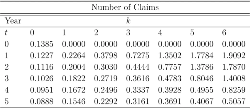
Let us now present the optimal BMS resulting from the four component Poisson mixture model. The NPMLE for this model led to a heterogeneous portfolio. There is one group which has a zero rate, also there is another group with very large rate (6.809), which however is only the 0.2% of the portfolio. The premiums that must be paid for various number of claims when the age of the policy is up to t=5 years will be determined by (8) and are presented in Table 2. From Table 2 we see that this optimal BMS is fair since if the policyholder has a claim free year the premium is reduced, while if the policyholder has one or more claims the premium is increased,resulting in bonus or malus respectively. Furthermore, we notice that this system can be considered generous with good risks and strict with bad risks.
Figure1a.pdfFigure1b.pdf
Figure 1: The gradient function for the data. The left plot shows the entire range while the right plot focuses on a smaller interval so as to provide a better picture
Table 1: Observed data and fitted probabilities with the associated 95% confidence intervals derived from the NPMLE using the quantile method.The observed data refer to a period of 3.5 years, so we also report annualized probabilities at the last 3 columns
Annualized
95% conf. int. 95% conf. int.
x observed rel. freq NPMLE LL UL mean LL UL 0 10441 0.667540 0.667540 0.645164 0.685471 0.878005 0.872903 0.883322 1 3604 0.230420 0.230541 0.203722 0.267963 0.107955 0.102907 0.113005 2 1108 0.070839 0.070366 0.054538 0.084995 0.012038 0.010155 0.013724 3 321 0.020523 0.021372 0.012489 0.026335 0.001640 0.001142 0.002166 4 109 0.006969 0.006452 0.003759 0.009697 0.000281 0.000096 0.000500 5 34 0.002174 0.001904 0.000798 0.004446 0.000059 0.000006 0.000157 ≥6 24 0.001534 0.001518 0.000319 0.004331 0.000022 0.000001 0.000105
Table 2: Optimal BMS with NPMLE Model Number of Claims Year k t 0 1 2 3 4 5 6 0 0.1385 0.0000 0.0000 0.0000 0.0000 0.0000 0.0000 1 0.1227 0.2264 0.3798 0.7275 1.3502 1.7784 1.9092 2 0.1116 0.2004 0.3030 0.4444 0.7757 1.3786 1.7870 3 0.1026 0.1822 0.2719 0.3616 0.4783 0.8046 1.4008 4 0.0951 0.1672 0.2496 0.3337 0.3928 0.4955 0.8259 5 0.0888 0.1546 0.2292 0.3161 0.3691 0.4067 0.5057
6.2
Confidence Intervals
We are interested in building confidence intervals for the premiums that must be paid by a policyholder who is observed for 5 years and whose number of claims range from 1 to 6. Firstly, Wald type two-sided intervals based on NPMLE are constructed according to (11) and are presented in Table 3. The NPMLE based approach provides smooth estimates of the posterior mean claim frequency leading to intervals of reasonable length. Nevertheless, the lower bounds of the intervals defined in (11) might be in some cases negative as they rely on the asymptotic
standard deviation estimates. On these occasions, NPMLE based CIs lie outside the admissible range since the premium rates must always be positive. In our application, negative lower CI bounds were observed for (t = 1, k = 6). For this purpose, in Table 3 this value is replaced by zero. Secondly, given our data, we generated B = 1000 bootstrap samplesNt,∗1 , ..., Nt,n∗ of size 15641 from ˆπ(k) in order to construct the Efron percentile bootstrap intervals based on (13). The results are presented in Table 4. It should be noted that all NPMLEs were computed without restriction to the support. This is because in Poisson mixtures the largest point in the support of an unrestricted NPMLE cannot be greater than the largest observation (see for example, Lindsay, 1995) and also because in theoretical results the interval [0, M], i.e. the support of Λ, may be fixed arbitrarily large (see Proposition 1 above, and Karlis and Patilea, 2008).
T able 3: NPMLE Based C I’s Num b er of Claims Y ear k t 0 1 2 3 4 5 6 0 [0 . 125066 , 0 . 151935] 0 . 000000 0 . 000000 0 . 000000 0 . 000000 0 . 000000 0 . 000000 1 [0 . 109660 , 0 . 135809] [0 . 185184 , 0 . 267589] [0 . 268289 , 0 . 491340] [0 . 282276 , 0 . 996328] [0 . 458679 , 1 . 953238] [0 . 747085 , 3 . 274443] [0 . 000000 , 5 . 814480] 2 [0 . 101249 , 0 . 121899] [0 . 175168 , 0 . 225622] [0 . 250150 , 0 . 355885] [0 . 332413 , 0 . 556384] [0 . 576910 , 0 . 974589] [1 . 059058 , 1 . 698085] [1 . 267187 , 2 . 306903] 3 [0 . 093517 , 0 . 111645] [0 . 161832 , 0 . 202639] [0 . 237686 , 0 . 306021] [0 . 293704 , 0 . 429557] [0 . 354031 , 0 . 602667] [0 . 617892 , 0 . 991348] [1 . 142949 , 1 . 658676] 4 [0 . 086998 , 0 . 103189] [0 . 148335 , 0 . 186124] [0 . 223511 , 0 . 275676] [0 . 288551 , 0 . 378911] [0 . 307061 , 0 . 478578] [0 . 355977 , 0 . 635075] [0 . 639244 , 1 . 012645] 5 [0 . 081636 , 0 . 095892] [0 . 135725 , 0 . 173462] [0 . 206673 , 0 . 251645] [0 . 282834 , 0 . 349452] [0 . 310256 , 0 . 427989] [0 . 310738 , 0 . 512743] [0 . 350130 , 0 . 661270] T able 4: Bo otstrap P ercen tile CI’s Num b er of Claims Y ear k t 0 1 2 3 4 5 6 0 [0 . 131961 , 0 . 144876] 0 . 000000 0 . 000000 0 . 000000 0 . 000000 0 . 000000 0 . 000000 1 [0 . 116414 , 0 . 129309] [0 . 187658 , 0 . 255338] [0 . 275891 , 0 . 551029] [0 . 324608 , 1 . 087990] [0 . 330889 , 2 . 233373] [0 . 332413 , 3 . 401027] [0 . 332446 , 3 . 677890] 2 [0 . 103606 , 0 . 122096] [0 . 147649 , 0 . 240049] [0 . 229204 , 0 . 417394] [0 . 277024 , 0 . 797113] [0 . 321135 , 1 . 247833] [0 . 332401 , 2 . 115248] [0 . 332444 , 2 . 936941] 3 [0 . 091261 , 0 . 119221] [0 . 128747 , 0 . 235845] [0 . 205423 , 0 . 349681] [0 . 236691 , 0 . 642096] [0 . 274231 , 0 . 956950] [0 . 321234 , 1 . 394413] [0 . 331201 , 2 . 095983] 4 [0 . 079151 , 0 . 117867] [0 . 118158 , 0 . 233527] [0 . 160054 , 0 . 311536] [0 . 214810 , 0 . 524566] [0 . 239658 , 0 . 843697] [0 . 270235 , 1 . 062482] [0 . 314374 , 1 . 534964] 5 [0 . 067264 , 0 . 117130] [0 . 110900 , 0 . 233524] [0 . 134524 , 0 . 282395] [0 . 204345 , 0 . 445821] [0 . 221954 , 0 . 719269] [0 . 240163 , 0 . 974344] [0 . 269635 , 1 . 183716]
Overall, from Tables 3 and 4 we observe that the Wald type intervals based on NPMLE, and the Efron bootstrap percentile intervals in most cases do not differ greatly. In both cases, a policyholder who is observed fort = 5 years of his presence in the portfolio and has a low claim frequency has a smaller confidence interval radius than one who in the same period of observation has more expected claims. For instance, when(t = 1, k = 2) the premium rates range from 0.26829 to 0.49134 and from 0.27589 to 0.55103, when (t = 4, k = 3) the premium rates range from 0.28855 to 0.37891 and from 0.21481 to0.52457, and when (t= 5, k= 5) the premium rates range from 0.31074 to 0.51274 and from 0.24016 to 0.97434 in the case of the Wald type intervals based on NPMLE and Efron bootstrap percentile intervals respectively. However, as we have already mentioned, for (t = 1, k = 6) the NPMLE based approach provides a very large and, thus, unusable CI. This aspect is improved by the bootstrap type interval which is not unreasonably long. The construction of confidence intervals is important because it indicates the precision of the estimates of the premiums of an optimal BMS. The reliability of the resulting premium estimates is bigger if the length of the intervals is smaller.
7
Conclusion
The present paper addressed the issue of building confidence intervals for the pre-miums determined by an optimal BMS, In this respect, actuarial literature research was extended since previous designs of such systems failed to identify customers with high claim frequency as they usually represent very few observations. Specifi-cally, NPML was used for estimating the risk distribution in a mixed Poisson model for the claim counts and this system was derived by means of the Bayes theorem, i.e. by updating the posterior mean claim frequency. As a result of the asymptotic normality of the estimator of the posterior mean claim frequency, Wald type two-sided confidence intervals were constructed. Such intervals are not degenerated and therefore are more useful than the corresponding intervals which could be derived from empirical estimation and those resulting from model based probability esti-mates that depend heavily on the form of the model under consideration. However, the construction of Wald type CIs relies on standard deviation estimates and thus in certain circumstances may have negative bounds, and as such prove to be larger than the nominal level. Therefore, the investigation was taken another step forward by considering the construction of Efron percentile bootstrap two-sided confidence intervals which was based on bootstrap from the NPMLE of the mixture. Efron type intervals require much more computing, but may make important improvements to
the asymptotic normal approximation used by Wald intervals. In an Bonus-Malus ratemaking scheme, the use of these intervals is beneficial for the insurance company as they account for the fluctuations in the imposed premiums. Moreover, their con-structions can be employed with flexibility by insurance companies which are free in a competitive market to set up their own tariff structures and rating policies.
Furthermore, we would like to emphasize that the interest is not on identifying risk groups. So using a smoother mixing distribution is not a key ingredient for our derivations, since we focus on the estimated claim distribution itself and not on the number of support points themselves. Also, the usage of covariate information for the model for a priori classification is under investigation. However, the derivation of the asymptotic normality is such cases is not straightforward and hence construction of confidence intervals needs further work.
Finally, a possible line of further research would be to employ nonparametric mix-tures of a multivariate Poisson distribution in order to construct an optimal BMS with a finite number of classes that takes into account different types of claims, for example claims with or without bodily injuries, or claims with full or partial liability of the insured driver. In this case, the independence assumption between claim types can be relaxed and it would be interesting to observe how the BMS might be affected. Moreover, one can investigate the asymptotic behaviour of the maximum likelihood estimators of the probabilities of a multivariate Poisson with a nonparametric mixing distribution. Specifically, if the asymptotic normality for the estimator of individual probabilities can be established, then following and extend-ing the framework of the present work, the NPML estimator can be used for the construction of confidence intervals for the premiums that must be paid for different types of claims.
Acknowledgments: We would like to thank the editor and the reviewer for
their constructive comments and suggestions.
Appendix A. Proof of Proposition 1
Fix kj ∈ N , the number of claims that the policyholder had in year j, j = 1, ..., t.
Then, K =
t P j=1
kj ,the total number of claims of a policyholder after t years of
insurance, will be a fixed value in N. Also, define the interval J = {K, K+ 1}
let ˆπ(K) and ˆπ(J) be the NPML estimators of πFΛ0(K) and πFΛ0(J) respectively.
Based on Corollary 2 of B¨ohning and Patilea (2005), which is an extension of Corol-lary 5.1 of Lambert and Tierney (1984), one can see that
√
n πˆ(J)−πFΛ0(J),πˆ(K)−πFΛ0(K)
=⇒N2((0,0),Ω (K)),
where N2 denotes a bivariate normal law and
Ω (K) = πFΛ0(J)−π 2 FΛ0(J) πFΛ0(J) 1−πFΛ0(K) πFΛ0(J) 1−πFΛ0(K) πFΛ0(K)−π2FΛ0(K) ! (A.1)
On the other hand, the premium that must be paid by this specific individual at
t+ 1 will be given λt+1(K) = ψ πFΛ0(J), πFΛ0 (K) , where ψ(x, y) = K+1 t x−y y .
Let ∇ψ(x, y) represent the vector of first-order partial derivatives of ψ(., .) at a point (x, y) with y 6= 0. The delta-method (see, for example, van der Vaart, 1998, Theorem 3.1) implies that
√ nλˆt+1(K)−λt+1(K) =⇒N(0, Vt+1(K)), (A.2) where Vt+1(K) = ∇ψ πFΛ0(J), πFΛ0(K) Ω (K)∇ψ πFΛ0 (J), πFΛ0(K) 0 = = 1 πFΛ0(K) ,−πFΛ0(J) π2 FΛ0(K) ! × πFΛ0(J)−π 2 FΛ0 (J) πFΛ0(J) 1−πFΛ0 (K) πFΛ0(J) 1−πFΛ0(K) πFΛ0(K)−πF2Λ0(K) ! × × 1 πFΛ0(K) −πFΛ0(J) π2 FΛ0(K) K + 1 t 2 = πFΛ0(J)πFΛ0(K) π3 FΛ0(K) K+ 1 t 2 = K+ 1 t 2"π FΛ0(K+ 1) π2 FΛ0(K) # " 1 + πFΛ0(K+ 1) πFΛ0(K) # .
Appendix B. Proof of asymptotic consistency of
Efron percentile bootstrap confidence intervals
Let us now provide a proof of the asymptotic consistency of the Efron percentile bootstrap interval (13) provided that the assumptions of Proposition 1 are satisfied. In what follows, fixkj ∈N, j = 1, ..., t,thus K ∈N is a fixed value, and define J as
in the previous proof. For eachl∈N, letp∗n(l) denote the proportion of observations equal to l in a bootstrap sample. Under the assumptions of Proposition 1, Karlis and Patilea (2008) showed that for anyl ∈N, if
R∗n(l) = √n(ˆπ∗(l)−p∗n(l)),
then for any δ > 0, P (|R∗n(l)|> δ|πˆ) → 0 in probability. From this, deduce that if ˆπ∗(J) = P l∈Jπˆ ∗(l) = ˆπ∗(K) + ˆπ∗(K+ 1), p∗ n(J) = P l∈Jp ∗ n(l) = p ∗ n(K) + p∗n(K+ 1) and R∗n=√n(ˆπ∗(K)−p∗n(K),πˆ∗(J)−p∗n(J)),
then for any δ > 0, P(kRn∗k> δ|πˆ) → 0 in probability. Based on the last display and using a central limit theorem for a triangular array (see, for instance, van der Vaart, 1998, pp. 20, 330–331) applied for the vector (p∗n(K), p∗n(J)), deduce that for any t1, t2 ∈R
P √n(ˆπ∗(K)−πˆ∗(K))≤t1,(ˆπ∗(J)−πˆ(J))≤t2|ˆπ
→F1(t1.t2),
where F1(., .) is the distribution function of a bivariate centered normal law with
the variance matrix Ω (K) given by (A.1).Working with subsequences along which the sequence√n(ˆπ∗(K)−πˆ∗(K),πˆ∗(J)−πˆ(J)) converges weakly to the bivariate normal law, conditionally, almost surely, using the delta method for bootstrap (see, for example,van der Vaart, 1998, Theorem 23.5) we deduce that for anyu∈R
√
nλˆ∗t+1(K)−λˆt+1(K)≤u|πˆ
→F2(u) in probability,
where F2(.) is the distribution function of the centered normal law with variance
Vt+1(K). Finally, the asymptotic consistency of the Efron percentile bootstrap
interval forλt+1(K) follows from the latter, the weak convergence (A.2) and Lemma
References
[1] B¨ohning, D. (2000). Computer-Assisted Analysis of Mixtures and Applications: Meta-Analysis, Disease Mapping and Others. Chapman and Hall, CRC, Lon-don.
[2] B¨ohning, D. and V. Patilea (2005). Asymptotic normality in mixtures of discrete distributions. Scandinavian Journal of Statistics, 32, 115–132.
[3] Boucher, J. P., M. Denuit and M. Guillen (2008). Models of Insurance Claim Counts with Time Dependence Based on Generalisation of Poisson and Negative Binomial Distributions. Variance, 2, 1, 135-162.
[4] Brouhns, N., M. Guillen, M. Denuit and J. Pinquet (2003). Bonus-malus scales in segmented tariffs with stochastic migration between segments. Journal of Risk and Insurance, 70, 577-599.
[5] Coene, G. and L.G. Doray (1996). A Financially Balanced Bonus-Malus System. ASTIN Bulletin, 26, 107-115.
[6] Denuit, M. and Ph. Lambert (2001). Smoothed NPML estimation of the risk distribution underlying Bonus-Malus systems. Proceedings of the Casualty Ac-tuarial Society, 88, 142–174.
[7] Denuit, M., Marechal, X., Pitrebois, S. Walhin, J. F. (2007). Actuarial mod-elling of claim counts: risk classification, and bonus-malus systems. Hoboken, NJ: Wiley.
[8] Dersimonian, R. (1986). Algorithm AS221 Maximum Likelihood Estimation of a Mixing Distribution. Applied Statistics, 35, 302-309.
[9] Dionne, G. and C. Vanasse (1989). A generalization of actuarial automobile insurance rating models: the negative binomial distribution with a regression component. ASTIN Bulletin, 19, 199-212.
[10] Dionne, G. and C. Vanasse (1992). Automobile insurance ratemaking in the presence of asymmetrical information. Journal of Applied Econometrics, 7, 149-165.
[11] Efron, B. (1982). The jackknife, the bootstrap and other resampling plans. Philadelphia, PA: CBMS 38. SIAM-NSF.
[12] Insurance Europe (2015). European Insurance Key Facts. Link: http://www.insuranceeurope.eu/sites/default/files/attachments/European %20Insurance%20-%20Key%20Facts%20-%20August%202015.pdf.
[13] Karlis, D. and V. Patilea (2007). Confidence Intervals of the hazard function for discrete distributions using mixtures. Computational Statistics and Data Analysis, 51, 5388-5401.
[14] Karlis, D. and V. Patilea (2008). Bootstrap confidence intervals intervals in mixtures of discrete distributions. Journal of Statistical Planning and Inference, 138, 2313-2329.
[15] Kestemont, R.M., and J. Paris (1985). Sur l’ajustement du Nombre de Sinistres. Bulletin of the Swiss Association of Actuaries, 157–163.
[16] Laird, N. (1978). Nonparametric Maximum Likelihood Estimation of a Mixing Distribution. Journal of the American Statistical Association, 73, 805-811. [17] Laird, N.M. and T.A. Louis (1987). Empirical Bayes confidence intervals based
on bootstrap samples (with discussion). Journal of the American Statistical Association, 82, 739–757.
[18] Lambert, D. and L. Tierney (1984). Asymptotic properties of the maximum likelihood estimates in mixed Poisson model. The Annals of Statistics, 12, 1388– 1399.
[19] Lesperance, M. and Kalbfleisch, J. (1992). An Algorithm for Computing the Nonparametric MLE of a Mixing Distribution. Journal of the American Statis-tical Association, 87, 120-126.
[20] Lindsay, B.G. (1983). The Geometry of Mixture Likelihood. A General Theory. The Annals of Statistics, 11, 86-94.
[21] Lindsay, B. G. (1995). Mixture models: theory, geometry and applications. NSF-CBMS regional conference series in probability and statistics, vol. 5. Hay-ward, CA: Institute of Mathematical Statistics and the American Statistical Association.
[22] Lindsay, B. G., and Lesperance, M. L. (1995). A review of semiparametric mixture models. Journal of Statistical Planning and Inference, 47(1), 29-39.
[23] Lemaire, J. (1995). Bonus-malus systems in automobile insurance. Norwell, MA: Kluwer Academic Publishers.
[24] Pinquet, J. (1998). Designing Optimal Bonus-Malus Systems From Different Types of Claims. ASTIN Bulletin, 28, 205-220.
[25] Pinquet, J., M. Guillen, and C. Bolance (2001). Long-range contagion in au-tomobile insurance data: estimation and implications for experience rating. ASTIN Bulletin, 31(2), 337-348.
[26] Pitrebois, S., M. Denuit, and JF. Walhin (2005). Bonus-malus systems with varying deductibles. ASTIN Bulletin, 35, 261–274.
[27] Simar, L., (1976). Maximum likelihood estimation of compound Poisson pro-cess. The Annals of Statistics, 4, 1200–1209.
[28] Tremblay, L. (1963). Using the Poisson-Inverse Gaussian distribution in Bonus-Malus Systems. ASTIN Bulletin, 22, 97–106.
[29] Tzougas,G.Frangos,N. (2014). The design of an optimal bonus-malus system-based on the Sichel distribution.Modern problems in insurance mathematics. New York: Springer Verlag.
[30] Tzougas, G., S, Vrontos and N. Frangos (2014). Optimal Bonus-Malus Systems Using Finite Mixture Models. ASTIN Bulletin, 44, 417-444.
[31] Walhin, J.-F., and J. Paris (1999). Using Mixed Poisson Distributions in Con-nection with Bonus-Malus Systems. ASTIN Bulletin, 29, 81–99.
[32] Wang, Y. (2007). On the fast computation of the nonparametric maximum likelihood estimate of a mixing distribution. Journal of the Royal Statistical Society, Series B, 69, 185-198.
[33] Willmot, G. E. (1987). The Poisson-inverse Gaussian distribution as an alter-native to the negative binomial. Scandinavian Actuarial Journal, 3-4, 113-127. [34] van de Geer, S. (1993). Hellinger-consistency of certain nonparametric
maxi-mum likelihood estimators. The Annals of Statistics, 21, 14-44.
[35] van der Vaart, A.W. (1998). Asymptotic Statistics. Cambridge University Press, Cambridge.