Estimating Adaptive Setpoint Temperatures Using Weather Stations

(1)

energies

Article

Estimating Adaptive Setpoint Temperatures Using

Weather Stations

David Bienvenido-Huertas1 , Carlos Rubio-Bellido2,* , Juan Luis Pérez-Ordóñez3 and Fernando Martínez-Abella3

1 _{Department of Graphical Expression and Building Engineering, University of Seville, 41012 Seville, Spain;} [email protected]

2 _{Department of Building Construction II, University of Seville, 41012 Seville, Spain}

3 _{Department of Civil Engineering, University of A Coruña, E.T.S.I. Caminos, Canales, Puertos Campus} Elviña s/n, 15071 La Coruña, Spain; [email protected] (J.L.P.-O.); [email protected] (F.M.-A.)

* Correspondence: [email protected]; Tel.: +34-686-135-595

Received: 9 February 2019; Accepted: 23 March 2019; Published: 27 March 2019

Abstract:Reducing both the energy consumption and CO2emissions of buildings is nowadays one of the main objectives of society. The use of heating and cooling equipment is among the main causes of energy consumption. Therefore, reducing their consumption guarantees such a goal. In this context, the use of adaptive setpoint temperatures allows such energy consumption to be significantly decreased. However, having reliable data from an external temperature probe is not always possible due to various factors. This research studies the estimation of such temperatures without using external temperature probes. For this purpose, a methodology which consists of collecting data from 10 weather stations of Galicia is carried out, and prediction models (multivariable linear regression (MLR) and multilayer perceptron (MLP)) are applied based on two approaches: (1) using both the setpoint temperature and the mean daily external temperature from the previous day; and (2) using the mean daily external temperature from the previous 7 days. Both prediction models provide adequate performances for approach 1, obtaining accurate results between 1 month (MLR) and 5 months (MLP). However, for approach 2, only the MLP obtained accurate results from the 6th month. This research ensures the continuity of using adaptive setpoint temperatures even in case of possible measurement errors or failures of the external temperature probes.

Keywords: adaptive setpoint temperature; weather station; multivariable linear regression; multilayer perceptron

1. Introduction

1.1. Energy Consumption of Residential Buildings

Global warming, resource depletion, extinction of species, and melting of glaciers constitute the main concerns faced by current society [1]. One of the main causes of such situations is the greenhouse gases emitted to the atmosphere due to the energy consumption from the most important industries and sectors. In this way, building sector is among those most contributing to this situation. Approximately, buildings are responsible for between 30% and 40% of the total energy consumption [2], emitting 40% of the total greenhouse gas emissions [3,4]. Also, social and health aspects, such as energy poverty [5] or the increase of the death rate because of high temperatures [6,7], also constitute worrying aspects to be solved. Consequently, institutions promote more and more the improvement of efficient energy of the existing buildings. The European Union has established goals to reduce the energy consumption and CO2emissions by 2020, although such goals are proving difficult to

(2)

achieve because both the measures adopted and the proximity of the deadline are not quite effective. Under this circumstance, the European Union has set a greater goal by 2050, with the aim of having a low-carbon economy [8].

The improvement of the energy performance has been traditionally focused on improving the envelope by reducing the thermal transmittance of its elements. However, the improvement of the performance and the use of HVAC systems have been scarcely studied, despite their high effect on the energy consumption of a building [9]. Likewise, the large number of buildings with HVAC systems is relevant to establish energy conservation measures. In Spain [10], more than 50% of buildings have envelopes with values of thermal transmittance meeting the state regulations [11]. Thus, the improvement of active systems in buildings with not enough effective systems or the improvement of their use can constitute possible energy conservation measures. In this research, given the influence of users on energy consumption [12], the decrease of such consumption is suggested by providing more adequate guidelines of using such systems, that is, by modifying the setpoint temperatures [13].

1.2. Adaptive Setpoint Temperatures

The influence of setpoint temperatures on the energy consumption has been analysed in many research studies: (i) Sánchez-García et al. [14] studied the use of a configuration of thermal comfort, which was different from that used by the regulation in Spain, as an energy conservation measure in office buildings. The results allowed the heating and cooling energy consumption to be reduced between 50% and 61%; (ii) in a later study, Sánchez-García et al. [13] analysed the potential of using mixed modes with adaptive setpoint temperatures in office buildings. The results allowed both the energy demand and energy consumption to be reduced by 74.6% and 59.7%, respectively, with respect to the reference model; (iii) Sánchez-Guevara Sánchez et al. [15] applied monthly variations of setpoint temperatures to a social housing, reducing the energy requirement between 20% and 80%; (iv) Spyropoulos and Balaras [16] evaluated the possibility of reducing the energy consumption in 39 bank branches in Greece by modifying the setpoint temperatures. A temperature of 26◦C for the upper limit and 20◦C for the lower limit resulted in a saving of 45% in the energy consumption; (v) Yun et al. [17] studied the improvement of using an adaptive comfort model in setpoint temperatures of office buildings. The energy consumption was decreased by 22%, and 87% of users had acceptable thermal comfort conditions; and (vi) Hoyt et al. [18] conducted a similar study in office buildings. The use of a setpoint temperature of 27.87◦C for cooling and 18.3◦C for heating reduced the energy consumption between 32% and 73%, according to the climate zone.

Residential buildings are characterized by combining the use of HVAC systems with natural ventilation (particularly in buildings located in warm regions). Natural ventilation is used when the external temperature values are acceptable. The HVAC system is used when external conditions exceed the limits of acceptability. Therefore, an energy saving can be achieved by using models of adaptive thermal comfort [14]. Such models are based on the natural tendency of people to adapt their clothing, metabolic rate, and psychological conditions to external climate variations under conditions of natural ventilation [19], thereby implying thermal comfort limits to be wider than those of the static models traditionally used [20].

One of the most developed models of adaptive thermal comfort is that included in EN 15251 [21]. This model can be used in those rooms occupied by users with a clothing level between 0.5 and 1 clo (1 clo = 0.155 (m2K)/W) and with a metabolic activity between 1 and 1.3 (1 met = 58 W/m2). The possibility of implementing such model is by modifying the setpoint temperatures of HVAC systems [14]. To do this, setpoint temperatures are adapted to the limits of the internal operative temperature (upper and lower) considered by EN 15251. This new setpoint temperature is known as adaptive setpoint temperature [14]. When the internal operative temperature is within the limits of EN 15251, active systems are not used, thus reducing the energy consumption. The use of such setpoint temperatures allows significant decreases to be obtained depending on the case study and the

(3)

Energies2019,12, 1197 3 of 47

climate zone [14,15,22]. The results show a decrease between 10% and 18% in the cooling consumption by using adaptive comfort models. To determine the limit values of EN 15251, the equations used are as follows: Trm= 0.2· n

∑

i=1 0.8i−1·Text,i (1) Ti,max = 0.33·Trm+18.8+γ (2) Ti,min= 0.33·Trm+18.8−γ (3)

whereTrmis the running mean temperature (◦C),Text,iis the external temperature from the previous dayiof the day when the running mean temperature (◦C) is calculated,Ti,max is the upper limit value of the internal operative temperature (◦C),Ti,max is the lower limit value of the internal operative temperature (◦C), andγis the value of the level of expectation (◦C). The value of the acceptability level is determined according to the category of intervention distinguished by EN 15251 (see Table1).

Table 1.Categories of EN 15251 and acceptability levels.

Categories Description γ

I High level of expectation. The standard recommends its use in buildings occupied by weak and sensitive people, with special requirements (e.g., sick people, children or elderly). 2 II Normal level of expectation. The standard recommends its use in new and renovated buildings. 3 III Moderate level of expectation. The standard recommends its use in existing buildings. 4

It is worth noting that adaptive setpoint temperatures are determined by using external temperature values. For their application to real cases, external temperature probes are required [14]. However, measuring the external temperature correctly can be a challenge. As it is known, any sensor installed in the exterior is at the mercy of being influenced by the external weather. The main causes for measurement errors in external temperature probes are the solar radiation and the wind [23]. The effect of the solar radiation is quite significant in probes because of the warming generated in the sensor [24–26]. Therefore, the error generated in the sensor increases as the solar radiation is higher [27]. Thus, the sensors installed in façades with a high solar radiation (e.g., façades facing east or west) can present distortions in measurements. Also, reflected radiation sources, such as the albedo of surfaces covered by snow [28,29] and the zenith angle of the sun [30,31], can also distort temperature measurements. Such measurement errors can be of several degrees [29,32,33].

The lack of radiant elements does not mean the lack of distortions in measurements. Even when there are robust instruments and no radiant elements affecting the probe, the measurement of the air temperature can be influenced by the wind action over the surface of the sensor, the existing vegetation, and close buildings [31,34]. Likewise, performing accurate measurements of the external air temperature is something of a challenge when there is a thermal gradient in a short distance, such as the existing area under the awning [35].

Thus, the implementation of adaptive setpoint temperatures in buildings can be limited if the external temperature probes are not installed under adequate conditions, or even if the probe gets damaged due to the lack of a good maintenance plan. This could result in a mistaken estimation of the adaptive setpoint temperatures. For this reason, new methodologies to determine the adaptive setpoint temperatures are suggested in this research. Data from weather stations of official meteorological agencies were used, thereby guaranteeing that data from installations do not present errors because of environmental aspects as well as that equipment is correctly installed thanks to the maintenance plans of such agencies. Also, adaptive setpoint temperatures are used without having external probes, thus ensuring both the economic saving in the investment and a greater implementation rate. To determine the adaptive setpoint temperatures, two different approaches were used, and two different regression algorithms (multivariable linear regression and multilayer perceptron) were in turn used in each approach.

(4)

This article is divided as follows: Section2describes the methodology, that is, characteristics of the equipment used, the approaches to determine the adaptive setpoint temperatures, the regression algorithms, and the procedures of training and validation of models. Section3discusses the results obtained. Finally, Section4summarizes the main conclusions.

2. Methodology 2.1. Case Study

Galicia is the autonomous community located in the northwest region of Spain (Figure1). This region covers an area of 29,575 km2, with a population of 2,701,743 people in 2018 [36,37]. In this area, the climate is oceanic Mediterranean (Csb) according to the Köppen-Geiger climate classification [38]. This climate typology is found in various other geographical points of the planet, such as Chile or the United States [38]. However, the climate in Galicia is influenced by the topography of the region. The topography significantly influences climate because precipitation pattern, relative humidity, temperatures, and solar radiation will vary according to the altitude [39–42]. Thus, in Galicia, where the altitude varies from 0 to more than 1000 m above sea level, there are various microclimates [43]. In this way, the Spanish Building Technical Code distinguishes six different climate zones according to the climate severity of winter and summer [11].

Energies 2019, 12, x FOR PEER REVIEW 5 of 47

different temperature distributions. With this aspect, the limitations that may exist in the methodologies used in case of using data from weather stations under different climate conditions were assessed.

Figure 1. Location of the case study and the weather stations used. Further information of the weather

stations can be found in Table 3.

Figure 2. Temperature probe of the case study.

Figure 1.Location of the case study and the weather stations used. Further information of the weather stations can be found in Table 3.

The case study is located in San Vicente de Elviña (Figure 1), at a latitude of 43.33001 and a longitude of−8.41179 (WGS84 coordinate system). It is at an altitude of 55 m. The temperature and the relative humidity were monitored using a CR1000 datalogger (Campbell Scientific, Logan,

(5)

Energies2019,12, 1197 5 of 47

UT, USA) with a HC2S3 sensor (Figure2). The technical specifications of the probe are indicated in Table2. The measurement interval was 30 min throughout almost 3 years (from 12 February 2016 to 17 December 2018). Each instance of the dataset was the average of 1800 measures. The sensor was placed in a pole closed to the wall of the case study, at a distance of 20 cm from the façade and 150 cm from the slab. The sensor was located facing north to avoid the effects of solar radiation [44]. Also, the sensor had a Campbell RAD10 multi-plate radiation shield. By obtaining the measurements of the external temperature, the adaptive setpoint temperatures (upper and lower limits) could be determined for categories I, II, and III from EN 15251.

different temperature distributions. With this aspect, the limitations that may exist in the methodologies used in case of using data from weather stations under different climate conditions were assessed.

Figure 1. Location of the case study and the weather stations used. Further information of the weather

stations can be found in Table 3.

Figure 2. _{Figure 2.}Temperature probe of the case study. _{Temperature probe of the case study.}

Table 2.Technical specifications of the external temperature probe used.

Technical Specification Values

Measurement Range −50 to 100◦C (default−40 to 60◦C)

Output Signal Range 0 to 1 V

Accuracy ±0.1◦C with standard configuration settings (at 23◦C)

Long-Term Stability <0.1◦C/year

2.2. Weather Stations

As mentioned in Section1, the objective of this research was determining adaptive setpoint temperatures without using external temperature probes. For this purpose, data from weather stations of an official meteorological agency, MeteoGalicia, were used. MeteoGalicia is a meteorological agency which is dependent of the Consellería de Medio Ambiente, Territorio e Infraestruturas of the Xunta de Galicia. Nowadays, such agency includes in its website a wide variety of environmental observation datasets from different weather stations.

The weather stations selected for this study were as follows: Coruña-Hércules, Coruña-Bens, Rio do Sol, A Gándara, Coto Muiño, Santiago EOAS, Sambreixo, Xesteiras, Cariño, and Salvora. From such stations, the values of the average daily temperature at 1.5 m, which were registered in the same test period that the case study, were compiled. As can be seen in Figure1and Table3, such weather stations were selected because they present important differences in the altitude and the distance between coordinates with respect to the case study. The average values of the daily external temperature had therefore differences with respect to the case study (Figure3). In this sense, the weather stations located in areas with a high altitude, such as Sambreixo or Xesteiras, presented different temperature distributions. With this aspect, the limitations that may exist in the methodologies used in case of using data from weather stations under different climate conditions were assessed.

(6)

Table 3.Coordinates of the weather stations. Weather Station Latitudea Longitudea Altitude

(m)

Distance from the Case Study (m)

Height Difference with Respect to the Case Study (m)

1. Coruña-Hercules 43.3829 −8.40993 21 5883.02 −34 2. Coruña-Bens 43.3634 −8.44187 131 4438.60 76 3. Rio do Sol 43.0952 −8.69099 540 34,549.61 485 4. A Gándara 43.1081 −9.05694 405 57,808.57 350 5. Coto Muiño 43.028873 −8.974914 317 56,622.68 262 6. Santiago EOAS 42,876 −8.55944 255 51,887.22 200 7. Sambreixo 43.1457 −7.79112 496 54,295.09 441 8. Xesteiras 42.6756 −8.58618 715 74,136.00 660 9. Cariño 43,734 −7.86335 5 63,029.12 −50 10. Salvora 42.4649 −9.01364 24 107,967.54 −31 a_{WGS84 coordinate system.}

Figure 3. Box-plots of the daily temperatures of the case study and the weather stations. The upper and bottom lines represent 25% of the data distribution of maximum and minimum values, respectively. The points are outliers in the data distribution.

Table 3. Coordinates of the weather stations. Weather Station Latitude a_Longitudea_Altitude_(m)Distance from the

Case Study (m)

Height Difference with Respect to the Case Study (m) 1. Coruña-Hercules 43.3829 −8.40993 21 5883.02 −34 2. Coruña-Bens 43.3634 −8.44187 131 4438.60 76 3. Rio do Sol 43.0952 −8.69099 540 34,549.61 485 4. A Gándara 43.1081 −9.05694 405 57,808.57 350 5. Coto Muiño 43.028873 −8.974914 317 56,622.68 262 6. Santiago EOAS 42,876 −8.55944 255 51,887.22 200 7. Sambreixo 43.1457 −7.79112 496 54,295.09 441 8. Xesteiras 42.6756 −8.58618 715 74,136.00 660 9. Cariño 43,734 −7.86335 5 63,029.12 −50 10. Salvora 42.4649 −9.01364 24 107,967.54 −31 a_{WGS84 coordinate system.}

The temperature values obtained by the weather stations were measured by using the sensors indicated in Table 4. Despite sensors are designed for being used under unfavourable external conditions (e.g., rainfalls or solar radiation), they were installed inside a protection box to guarantee that the data registered by the sensors of each weather stations did not present errors.

Figure 3.Box-plots of the daily temperatures of the case study and the weather stations. The upper and bottom lines represent 25% of the data distribution of maximum and minimum values, respectively. The points are outliers in the data distribution.

The temperature values obtained by the weather stations were measured by using the sensors indicated in Table4. Despite sensors are designed for being used under unfavourable external conditions (e.g., rainfalls or solar radiation), they were installed inside a protection box to guarantee that the data registered by the sensors of each weather stations did not present errors.

(7)

Energies2019,12, 1197 7 of 47

Table 4.Temperature and humidity sensors of each weather station.

Sensor Measurement Range Accuracy Weather Station

Vaisala HMP155 −80–60◦C ±0.25◦C Coruña-Hércules, Coruña-Bens, Rio do Sol, A Gándara, Coto Muiño, Sambreixo, Cariño, Salvora Geónica STH-5031 −40–60◦C ±0.10◦C Santiago EOAS

Rotronic HC2A-S3 −50–100◦C ±0.30◦C Xesteiras

2.3. Approaches for Estimating Adaptive Setpoint Temperatures

To estimate the adaptive setpoint temperatures, two approaches were designed (Table 5): (i) approach 1, where the adaptive setpoint temperature is determined with the adaptive setpoint temperature from the previous day and the mean daily external temperature from the previous day of the weather station; and (ii) approach 2, where the adaptive setpoint temperature is determined with the mean daily temperatures of the 7 previous days. Such approaches were designed in accordance with criteria from EN 15251 to estimate the limits of adaptive thermal comfort. Moreover, they were designed to estimate both upper and lower limits. Input and output variables were used by the regression algorithms described in Section2.4to generate prediction models of each weather station.

Table 5.Input and output variables for each approach.

Approach Input Variables Output Variables

Approach 1 Text,d−1,Tsp,d−1a Tsp,da

Approach 2 Text,d−1,Text,d−2,Text,d−3,Text,d−4,Text,d−5,Text,d−6,Text,d−7 Tsp,da

Text,d−n: mean daily external temperature from the previousndays;Tsp,d−1: adaptive setpoint temperature from the previous day;Tsp,d: adaptive setpoint temperature from the current day. aAdaptive setpoint temperature corresponding to the upper and lower limit. Regarding approach 1, the limit of the adaptive setpoint temperature will be the same for both input and output variable.

2.4. The Regression Algorithms Used

To generate the prediction models, two regression algorithms were used: a multivariable linear regression (MLR) and a multilayer perceptron (MLP).

2.4.1. MLR

MLR is a classic regression algorithm which connects a dependent variable (yi) with independent variablesp:

yi= β0+

∑

βpXpi+εi (4)

whereXpiare the independent variables (also called explicative),pis the number of the independent variables,β0is the constant term,βpis the influence of variables on the dependent variable, andεiis the term of error (also called term of noise).

MLR is based on a linear statistical model without needing adjustment parameters, and this is an advantage by applying it [45]. Another advantage is understanding the existing relationship between the independent variables and the dependent variable [46]. Such algorithm has therefore been widely used to estimate and predict in the energy analysis of buildings: (i) Pulido-Arcas et al. [46] developed 18 MLRs to estimate the energy consumption and CO2 emissions in office buildings which were located in 9 cities of Chile. The correlation coefficient obtained by the models ranged between 91.81% and 99.56%, thereby reflecting the possibilities of using such models for the energy characterization of office buildings; (ii) Qiang et al. [47] developed MLR models to estimate the daily mean cooling load in HVAC systems of office buildings in Tianjin (China). The estimations obtained by the models presented a mean absolute percentage error lower than 8% with respect to the real values; (iii) Amber et al. [48] developed an MLR to estimate the daily energy consumption in university buildings. The independent variables of the model were external temperature, relative humidity, solar

(8)

radiation, wind speed, weekday index (1 for working days and 0 for the remaining days), and type of building. The results obtained error parameters between 12% and 13% according to the type of building analysed; (iv) a wider approach was given by Kialashaki and Reisel [49]. These authors developed MLRs to estimate the energy demand of the residential building stock in United States. The performance of the models obtained correlation coefficients greater than 95%; and (v) the problem of reducing the energy consumption in the design phase was analysed by Asadi et al. [50]. In such study, the use of MLRs to estimate the energy consumption of commercial buildings was assessed by using the input variables of the envelope and the morphology of the building, as well as the building occupancy schedule.

2.4.2. MLP

MLPs simulate, through mathematical models, the behaviour of the nervous system. As in the biological model, the artificial neuron is in charge of receiving, processing, and transmitting information to the following multiple neurons [51]. The output information is obtained from the processing through the network of the input information (Figure4). To integrate and compute the information from the environment and other neurons, the artificial neuron uses the propagation, activation, and transfer function. Generally, the propagation function (Equation (5)) is the sum of each input (pj) multiplied by a weight (Wij):

nj= n−1

∑

i=0

Wjipi (5)

humidity, solar radiation, wind speed, weekday index (1 for working days and 0 for the remaining days), and type of building. The results obtained error parameters between 12% and 13% according to the type of building analysed; (iv) a wider approach was given by Kialashaki and Reisel [49]. These authors developed MLRs to estimate the energy demand of the residential building stock in United States. The performance of the models obtained correlation coefficients greater than 95%; and (v) the problem of reducing the energy consumption in the design phase was analysed by Asadi et al. [50]. In such study, the use of MLRs to estimate the energy consumption of commercial buildings was assessed by using the input variables of the envelope and the morphology of the building, as well as the building occupancy schedule.

2.4.2. MLP

MLPs simulate, through mathematical models, the behaviour of the nervous system. As in the biological model, the artificial neuron is in charge of receiving, processing, and transmitting information to the following multiple neurons [51]. The output information is obtained from the processing through the network of the input information (Figure 4). To integrate and compute the information from the environment and other neurons, the artificial neuron uses the propagation, activation, and transfer function. Generally, the propagation function (Equation (5)) is the sum of each input ( ) multiplied by a weight ( ):

= (5)

Figure 4. Example of an MLP of a hidden layer.

The activation function ( ) modifies the value obtained in the propagation function (Equation (6)), thus relating the input of each neuron to the next activation state. At the output of the neuron, there could be a threshold function establishing a limit value, which should be exceeded before being propagated to another neuron (Equation (7)). This function is known as the transfer function ( ). The next point to define an MLP is to determine the network topology to be used. MLPs are mainly divided into feedforward and feedback networks. The first network moves the information to a single direction (input towards output), and the second to any direction:

( ) = ( − 1), ( − 1) (6)

= ( ) (7)

where ( − 1) is the input value of the neuron, is the activation value, and is the iteration. MLPs constitute nowadays one of the most used regression algorithms because they generally have a better performance than other regression algorithms [52,53]. In consequence, they have been used in many research works to assess the energy performance of buildings and installations: (i) Attoue et al. [54] developed a model of artificial neural network to estimate the variation of the internal temperature so that the energy consumption in the building could be optimized. By using

Figure 4.Example of an MLP of a hidden layer.

The activation function (AF) modifies the value obtained in the propagation function (Equation (6)), thus relating the input of each neuron to the next activation state. At the output of the neuron, there could be a threshold function establishing a limit value, which should be exceeded before being propagated to another neuron (Equation (7)). This function is known as the transfer function (TF). The next point to define an MLP is to determine the network topology to be used. MLPs are mainly divided into feedforward and feedback networks. The first network moves the information to a single direction (input towards output), and the second to any direction:

ai(t) = AF(ai(t−1), ni(t−1)) (6)

outi= TF(ai(t)) (7)

wherenj(t−1)is the input value of the neuron,ajis the activation value, andtis the iteration. MLPs constitute nowadays one of the most used regression algorithms because they generally have a better performance than other regression algorithms [52,53]. In consequence, they have been used in many research works to assess the energy performance of buildings and installations: (i) Attoue et al. [54] developed a model of artificial neural network to estimate the variation of the

(9)

Energies2019,12, 1197 9 of 47

internal temperature so that the energy consumption in the building could be optimized. By using the three-hour façade temperature history and the external temperature as input variables, the internal temperature could be suitably estimated until two hours after obtaining the input data; (ii) Zabada and Shahrour [55] carried out an analysis using an artificial neural network to assess the influence of different parameters on heating cases in social dwellings in France. Such analysis reflected that some parameters, such as the surface of the dwelling, date of construction, and the energy performance, influenced the heating consumption. Likewise, social indicators such as family size, member age, and tenant income influenced the heating expense; (iii) Yu et al. [56] developed an MLP to estimate the heating energy demand in residential buildings. The model was validated with actual demand values in residential buildings of Chongqing (China). The errors of the estimation obtained by the model were lower than±2.5%; (iv) a similar approach was carried out by Deb et al. [57] to estimate the diurnal cooling load in institutional buildings. The MLP developed allowed the cooling loads in the following 20 days to be accurately predicted; and (v) Moon et al. [58] developed an MLP for the thermal control in buildings with double skin envelopes by using the air gap temperature and the internal and external air temperatures, among others, as input variables. The performance of the MLP was analysed for several opening strategies in heating or cooling situations.

2.5. Dataset, Training, and Testing of the Models

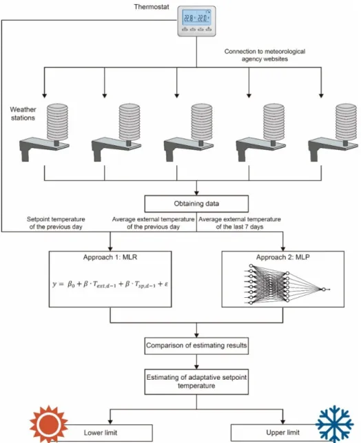
The development, validation, and testing of the approaches and the prediction models followed the flowchart of Figure5. Firstly, measurements performed by the external probe of the case study and the weather stations of MeteoGalicia were compiled. Then, adaptive setpoint temperatures of the 3 categories from EN 15251 (Equations (1)–(3)) were determined. The running mean temperature was obtained through data of the temperature probe of the case study. It is worth highlighting that the limit value obtained from Equations (2) and (3) (e.g., for the upper limit of category III, temperatures of 26.10 and 32.70 were used for their minimum and maximum values, respectively) was used in those cases in that the running mean temperature is not within the application of the standard (i.e., when such temperature is not between 10 and 30◦C for the upper limit, and not between 15 and 30◦C for the lower limit).

The full dataset was generated by using such data, with a total of 1040 instances (measurement days). Both the training and testing dataset were generated with such dataset (Table6). The training datasets were used to generate individual models for each weather station as well as for each limit of adaptive setpoint temperature (upper or lower), using MLR or MLP as regression algorithms. To generate the MLR models, the Akaike information criterion was used [59].

Table 6.Datasets used.

Dataset Number of Instances (days) First Date Last Date

Training 365 12 February 2016 11 February 2017

Testing 675 12 February 2017 17 December 2018

For the MLPs, only architectures of three layers (input, hidden, and output layers) were used because they generally have performances better than more complex architectures [60]. The sigmoid function has been selected as a transfer function. In the training of the MLPs, the Broyden-Fletcher-Goldfarb-Shanno (BFGS) algorithm [61] has been chosen, thus minimizing the mean squared error of the difference between the outputs in each step. Likewise, the training was carried out using a 10-fold cross validation, thereby dividing randomly the training dataset into 10 subsets: for each fold, 9 subsets were used as a training dataset, and the remaining subset was used to assess the performance of each model. Through this procedure, both the error and the variance of the model decreased [62].

The testing dataset was used to determine the error of generalization of the models obtained in the training phase. The performance of each model was assessed by analysing three quality statistical

(10)

parameters: the linear correlation coefficient (R2) (Equation (8)), the mean absolute error (MAE) (Equation (9)), and the root mean square error (RMSE) (Equation (10)):

R2= 1−∑ n i=1(ti−mi)2 ∑n i=1 ti−ti 2 ! (8) MAE= ∑ n i=1|ti−mi| n (9) RMSE= ∑ n i=1(ti−mi)2 n !1/2 (10) wheremiis the model’s estimation,tiis the actual value of adaptive setpoint temperature, andnis the number of observations in the dataset.

= 1 −∑_∑ ( −_{( − ̅ )}) (8)

=∑ | − | (9)

= ∑ ( − )

/

(10) where is the model’s estimation, is the actual value of adaptive setpoint temperature, and is the number of observations in the dataset.

Figure 5. Flowchart of this research. 3. Results and Discussion

After generating the dataset, the estimation models were analysed. This section is structured by distinguishing the approach used and the performance obtained by the MLR and MLP models in each of them. As mentioned in Section 2.5, all models were created by using a training dataset of 1 year, and the testing dataset corresponds to the remaining period of time (675 days). Based on the similarity of the results of the statistical parameters of the models for the three categories of EN 15251, the values of category III are indicated in the following tables to make its reading easier because variations presented by the statistical parameters between the different categories were lower than 2%. Appendix A shows the point clouds between the actual and estimated values for the different categories so that the reader can visualize the accuracy level of the estimations performed by each model.

Figure 5.Flowchart of this research.

3. Results and Discussion

After generating the dataset, the estimation models were analysed. This section is structured by distinguishing the approach used and the performance obtained by the MLR and MLP models in each of them. As mentioned in Section2.5, all models were created by using a training dataset of 1 year, and the testing dataset corresponds to the remaining period of time (675 days). Based on the similarity of the results of the statistical parameters of the models for the three categories of EN 15251, the values of category III are indicated in the following tables to make its reading easier because variations presented by the statistical parameters between the different categories were lower than 2%. AppendixAshows the point clouds between the actual and estimated values for the different categories so that the reader can visualize the accuracy level of the estimations performed by each model.

(11)

Energies2019,12, 1197 11 of 47

3.1. Approach 1: With the Setpoint Temperature and the External Temperature from the Previous Day As mentioned above, this approach consisted of determining the adaptive setpoint temperature with external temperature data from the previous day(Text,d−1)and the adaptive setpoint temperature from the previous dayTsp,d−1

. Depending on the limit to be estimated (upper or limit), the setpoint temperature from the previous day for such limit is used.

It is worth noting the importance of using the setpoint temperature from the previous day. Such temperature was used because it generated an adjustment degree on the models. In this sense, Figures6 and7show how includingTsp,d−1generated a high adjustment between the actual and the estimated values. Despite the high adjustment obtained withTsp,d−1,Text,d−1is required to be considered as an independent variable because it reduces the error related to the estimations when the external temperature fluctuations are presented.

3.1. Approach 1: With the Setpoint Temperature and the External Temperature from the Previous Day As mentioned above, this approach consisted of determining the adaptive setpoint temperature

with external temperature data from the previous day , and the adaptive setpoint

temperature from the previous day , . Depending on the limit to be estimated (upper or limit), the setpoint temperature from the previous day for such limit is used.

It is worth noting the importance of using the setpoint temperature from the previous day. Such temperature was used because it generated an adjustment degree on the models. In this sense, Figures

6 and 7 show how including , generated a high adjustment between the actual and the

estimated values. Despite the high adjustment obtained with , , , is required to be

considered as an independent variable because it reduces the error related to the estimations when the external temperature fluctuations are presented.

3.1.1. MLR

First, the performance of approach 1 was analysed using the MLR as a regression algorithm. Table 7 indicates the performances obtained by the MLRs, and Figures A1–A3 and A13–A15 in Appendix A show the point clouds between the actual and the estimated values of the different categories from EN 15251. As can be seen, the performance obtained by the MLRs was quite adjusted. In this sense, was always greater than 99% both in the training and the testing of the upper and lower limits. There were no great deviations in the estimation of the limit values (values which are not within the application of the standard), with a mean deviation value of 0.06 °C in these

temperatures. Also, and were lower than 0.10 and 0.15, respectively, in the testing

phase of almost all models, and only in some cases the error parameters were higher than these two values, although the increase in the error parameters was always lower than 25%. By using data from distant weather stations, a lower performance was not detected either. As seen in Section 2.2, the weather stations of Sambrexio, Xesteiras, Cariño, and Salvora were those more distant from the case study. The performances of the models generated with data from such weather stations were analysed, and the results obtained were similar to those from other nearer weather stations, even obtaining better performances (e.g., the MLPs of the weather station of Sambreixo, with statistical parameters better than those of the weather stations of Rio do Sol and A Gándara). Only the MLPs of the weather station of Xesteiras obtained a less adjusted performance than the other models, although the correlation coefficient was greater than 99%.

Figure 6. Influence of applying the setpoint temperature from the previous day on the MLR by using the external temperature of the weather station of Xesteiras.

Figure 6.Influence of applying the setpoint temperature from the previous day on the MLR by using the external temperature of the weather station of Xesteiras.Energies 2019, 12, x FOR PEER REVIEW 12 of 47

Figure 7. Influence of applying the setpoint temperature from the previous day on the MLP by using the external temperature of the weather station of Xesteiras.

Table 7. Results of the training and testing of the MLR models of approach 1. Model Upper Limit Lower Limit

Training Coruña-Hercules 99.71 0.0696 0.0911 99.01 0.0654 0.0936 Coruña-Bens 99.70 0.0694 0.0923 99.10 0.0650 0.0895 Rio do Sol 99.51 0.0887 0.1183 99.04 0.0640 0.0921 A Gándara 99.54 0.0876 0.1147 99.06 0.0642 0.0915 Coto Muiño 99.72 0.0689 0.0903 99.07 0.0649 0.0908 Santiago EOAS 99.72 0.0675 0.0901 99.07 0.0641 0.0911 Sambreixo 99.66 0.0774 0.0984 99.05 0.0651 0.0919 Xesteiras 99.36 0.1006 0.1356 99.00 0.0642 0.0940 Cariño 99.58 0.0815 0.1099 98.96 0.0643 0.0959 Salvora 99.71 0.0696 0.0911 99.01 0.0654 0.0936 Testing Coruña-Hercules 99.61 0.0774 0.1087 99.18 0.0679 0.0956 Coruña-Bens 99.52 0.1249 0.1525 99.22 0.0695 0.0954 Rio do Sol 99.53 0.0906 0.1218 99.21 0.0674 0.0937 A Gándara 99.54 0.0927 0.1209 99.21 0.0671 0.0941 Coto Muiño 99.76 0.0654 0.0853 99.27 0.0659 0.0905 Santiago EOAS 99.76 0.0649 0.0849 99.25 0.0667 0.0915 Sambreixo 99.61 0.0796 0.1077 99.17 0.0695 0.0964 Xesteiras 99.46 0.0999 0.1291 99.20 0.0671 0.0948 Cariño 99.62 0.0830 0.1076 99.11 0.0709 0.0999 Salvora 99.61 0.0774 0.1087 99.18 0.0679 0.0956

Another aspect to be considered was the minimum size of the training dataset to obtain valid results in the next months. Figure 8 shows how estimations with greater than 95% and values of and lower than 0.11 and 0.19, respectively, were obtained by using training sample of only a month. Moreover, the performance obtained was almost the same compared with the model generated with a training dataset of 1 year. The only requirement to obtain an accurate estimation is that the training period of 1 month is not composed only by days which are not within the limits of application (i.e., when the running mean temperature is not between 15 and 30 °C for the upper limit,

Figure 7.Influence of applying the setpoint temperature from the previous day on the MLP by using the external temperature of the weather station of Xesteiras.

(12)

3.1.1. MLR

First, the performance of approach 1 was analysed using the MLR as a regression algorithm. Table7indicates the performances obtained by the MLRs, and FiguresA1–A3and FiguresA13–A15 in AppendixAshow the point clouds between the actual and the estimated values of the different categories from EN 15251. As can be seen, the performance obtained by the MLRs was quite adjusted. In this sense,R2_{was always greater than 99% both in the training and the testing of the upper and lower} limits. There were no great deviations in the estimation of the limit values (values which are not within the application of the standard), with a mean deviation value of 0.06◦C in these temperatures. Also, MAEandRMSEwere lower than 0.10 and 0.15, respectively, in the testing phase of almost all models, and only in some cases the error parameters were higher than these two values, although the increase in the error parameters was always lower than 25%. By using data from distant weather stations, a lower performance was not detected either. As seen in Section2.2, the weather stations of Sambrexio, Xesteiras, Cariño, and Salvora were those more distant from the case study. The performances of the models generated with data from such weather stations were analysed, and the results obtained were similar to those from other nearer weather stations, even obtaining better performances (e.g., the MLPs of the weather station of Sambreixo, with statistical parameters better than those of the weather stations of Rio do Sol and A Gándara). Only the MLPs of the weather station of Xesteiras obtained a less adjusted performance than the other models, although the correlation coefficient was greater than 99%.

Table 7.Results of the training and testing of the MLR models of approach 1.

Model

Upper Limit Lower Limit

R2 MAE RMSE R2 MAE RMSE

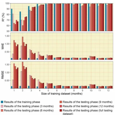
Another aspect to be considered was the minimum size of the training dataset to obtain valid results in the next months. Figure8shows how estimations withR2greater than 95% and values of MAEandRMSElower than 0.11 and 0.19, respectively, were obtained by using training sample of only a month. Moreover, the performance obtained was almost the same compared with the model generated with a training dataset of 1 year. The only requirement to obtain an accurate estimation is that the training period of 1 month is not composed only by days which are not within the limits of application (i.e., when the running mean temperature is not between 15 and 30◦C for the upper limit, and not between 10 and 30◦C for the lower limit). This aspect is quite relevant because, if the HVAC

(13)

Energies2019,12, 1197 13 of 47

system has an external temperature probe to record external temperatures, the predictive model could be generated by using data of a month, so the continuity of using adaptive setpoint temperatures is ensured even if the probe fails in a short period of time.

and not between 10 and 30 °C for the lower limit). This aspect is quite relevant because, if the HVAC system has an external temperature probe to record external temperatures, the predictive model could be generated by using data of a month, so the continuity of using adaptive setpoint temperatures is ensured even if the probe fails in a short period of time.

Figure 8. Influence of the size of the training sample on the MLR model (approach 1).

3.1.2. MLP

Despite the high performance obtained by the MLRs in approach 1, the MLPs were also analysed. Table 8 indicates the values of statistical parameters obtained in the training and testing phases of the different models.

Table 8. Results of the training and testing of the MLP models of approach 1.

Model Upper Limit Lower Limit

Training Coruña-Hercules 99.26 0.1112 0,146 98.99 0.0629 0.0969 Coruña-Bens 99.25 0.1117 0.1463 99.00 0.0623 0.0956 Rio do Sol 99.24 0.1100 0.1480 99.01 0.0596 0.0940 A Gándara 99.19 0.1144 0.1521 98.98 0.0619 0.0956 Coto Muiño 99.28 0.1089 0.1437 99.03 0.0591 0.0932 Santiago EOAS 99.31 0.1073 0.1410 99.12 0.0595 0.0899 Sambreixo 99.34 0.1051 0.1380 99.06 0.0606 0.0917 Xesteiras 99.13 0.1168 0.1575 98.88 0.0627 0.0998 Cariño 99.21 0.1143 0.1505 98.92 0.0659 0.0980 Salvora 99.26 0.1112 0.1459 98.99 0.0640 0.0973 Testing Coruña-Hercules 99.31 0.1197 0,157 99.18 0.0743 0.1072 Coruña-Bens 99.39 0.1158 0.1499 99.07 0.1123 0.1604 Rio do Sol 99.30 0.1313 0.1638 99.15 0.0790 0.1108 A Gándara 99.31 0.1284 0.1621 99.13 0.0743 0.1102 Coto Muiño 99.42 0.1260 0.1624 99.28 0.0830 0.1032 Santiago EOAS 99.46 0.1108 0.1438 99.34 0.0733 0.0961 Sambreixo 99.40 0.1414 0.1805 99.31 0.0808 0.1008 Xesteiras 99.30 0.1260 0.1610 99.18 0.0763 0.1057 Cariño 99.38 0.1252 0.1554 99.16 0.0770 0.1146 Salvora 99.31 0.1202 0.1581 99.19 0.0707 0.0998

Figure 8.Influence of the size of the training sample on the MLR model (approach 1). 3.1.2. MLP

Despite the high performance obtained by the MLRs in approach 1, the MLPs were also analysed. Table8indicates the values of statistical parameters obtained in the training and testing phases of the different models.

Table 8.Results of the training and testing of the MLP models of approach 1.

Model

Training Coruña-Hercules 99.26 0.1112 0,146 98.99 0.0629 0.0969 Coruña-Bens 99.25 0.1117 0.1463 99.00 0.0623 0.0956 Rio do Sol 99.24 0.1100 0.1480 99.01 0.0596 0.0940 A Gándara 99.19 0.1144 0.1521 98.98 0.0619 0.0956 Coto Muiño 99.28 0.1089 0.1437 99.03 0.0591 0.0932 Santiago EOAS 99.31 0.1073 0.1410 99.12 0.0595 0.0899 Sambreixo 99.34 0.1051 0.1380 99.06 0.0606 0.0917 Xesteiras 99.13 0.1168 0.1575 98.88 0.0627 0.0998 Cariño 99.21 0.1143 0.1505 98.92 0.0659 0.0980 Salvora 99.26 0.1112 0.1459 98.99 0.0640 0.0973 Testing Coruña-Hercules 99.31 0.1197 0,157 99.18 0.0743 0.1072 Coruña-Bens 99.39 0.1158 0.1499 99.07 0.1123 0.1604 Rio do Sol 99.30 0.1313 0.1638 99.15 0.0790 0.1108 A Gándara 99.31 0.1284 0.1621 99.13 0.0743 0.1102 Coto Muiño 99.42 0.1260 0.1624 99.28 0.0830 0.1032 Santiago EOAS 99.46 0.1108 0.1438 99.34 0.0733 0.0961 Sambreixo 99.40 0.1414 0.1805 99.31 0.0808 0.1008 Xesteiras 99.30 0.1260 0.1610 99.18 0.0763 0.1057 Cariño 99.38 0.1252 0.1554 99.16 0.0770 0.1146 Salvora 99.31 0.1202 0.1581 99.19 0.0707 0.0998

(14)

Also, the adjustment degree of the estimated values for each instance of the testing dataset is shown in AppendixA(Figures A4–A6 and FiguresA16–A18). As can be seen, the performance obtained was similar to that of the MLRs:R2was greater than 99%, andMAEandRMSEwere lower than 0.10 and 0.15, respectively. Likewise, differences between the models of weather stations nearer or more distant from the case study were not detected, and identical results were obtained for the models of categories I and II. Apart from such similarity between the MLRs and MLPs of approach 1, there is a difference between both models that can limit the use of the MLPs: the size of the training dataset. As can be seen in Figure9, the minimum size of a training dataset to obtain an acceptable performance is of 5 months, although increasing the training sample in 11–12 months would allow a greater stability in predictions to be guaranteed. In this sense, as can be proved in models of Table8(generated with a training dataset of 1 year), the performance of the estimations in the 675 days which composed the testing dataset was quite adjusted. Given that both the MLRs obtained similar performances and the minimum size of the training dataset for the MLRs is lower (1 month), the MLRs are therefore more possible to be used than the MLPs.

Also, the adjustment degree of the estimated values for each instance of the testing dataset is shown in Appendix A (Figures A4–A6 and A16–A18). As can be seen, the performance obtained was similar to that of the MLRs: was greater than 99%, and and were lower than 0.10 and 0.15, respectively. Likewise, differences between the models of weather stations nearer or more distant from the case study were not detected, and identical results were obtained for the models of categories I and II. Apart from such similarity between the MLRs and MLPs of approach 1, there is a difference between both models that can limit the use of the MLPs: the size of the training dataset. As can be seen in Figure 9, the minimum size of a training dataset to obtain an acceptable performance is of 5 months, although increasing the training sample in 11–12 months would allow a greater stability in predictions to be guaranteed. In this sense, as can be proved in models of Table 8 (generated with a training dataset of 1 year), the performance of the estimations in the 675 days which composed the testing dataset was quite adjusted. Given that both the MLRs obtained similar performances and the minimum size of the training dataset for the MLRs is lower (1 month), the MLRs are therefore more possible to be used than the MLPs.

Figure 9. Influence of the size of the training sample on the MLP model (approach 1).

3.2. Approach 2: With Average Temperatures of the Last Seven Days

As mentioned in Section 2.3, this approach consisted of determining the adaptive setpoint temperature of the upper and lower limits by using external temperature data from the previous 7

days , , , , , , , , , , , , , . It was necessary to consider using

the 7 external temperatures from the previous days because their performance improved for the MLR models (Figure 10) and the MLP models (Figure 11) by increasing the number of input variables.

Figure 9.Influence of the size of the training sample on the MLP model (approach 1). 3.2. Approach 2: With Average Temperatures of the Last Seven Days

As mentioned in Section 2.3, this approach consisted of determining the adaptive setpoint temperature of the upper and lower limits by using external temperature data from the previous 7 days(Text,d−1,Text,d−2,Text,d−3,Text,d−4,Text,d−5,Text,d−6,Text,d−7). It was necessary to consider using the 7 external temperatures from the previous days because their performance improved for the MLR models (Figure10) and the MLP models (Figure11) by increasing the number of input variables. 3.2.1. MLR

As in the models of approach 1, the performance of the models of the different weather stations was first assessed for the adaptive setpoint temperatures of categories I, II, and III.

(15)

Energies2019,12, 1197 15 of 47

Figure 10. Influence of the number of the external temperatures used on the MLR model of A Gándara. Values obtained from the training of the model of the upper limit.

Figure 11. Influence of the number of the external temperatures used on the MLP model of A Gándara. Values obtained from the training of the model of the upper limit.

3.2.1. MLR

Table 9. Results of the training and testing of the MLR models of approach 2. Model Upper Limit Lower Limit Training Coruña-Hercules 98.20 0.1621 0.2251 85.25 0.2865 0.3490 Coruña-Bens 97.97 0.1747 0.2389 86.03 0.2835 0.3404 Rio do Sol 94.04 0.3138 0.4057 83.03 0.2965 0.3721 A Gándara 94.42 0.3026 0.3930 83.25 0.2947 0.3699 Coto Muiño 98.44 0.1523 0.2100 87.45 0.2686 0.3238 Santiago EOAS 97.69 0.1952 0.2548 87.31 0.2637 0.3255 Sambreixo 97.96 0.1843 0.2398 87.11 0.2688 0.3279 Xesteiras 90.88 0.3859 0.4978 81.60 0.2993 0.3860 Cariño 97.00 0.2173 0.2903 87.06 0.2652 0.3285 Salvora 98.20 0.1621 0.2251 85.25 0.2865 0.3490 Testing Coruña-Hercules 97.35 0.2039 0.3017 86.04 0.3300 0.3884 Coruña-Bens 96.91 0.4471 0.5543 91.03 0.2769 0.3434 Rio do Sol 97.71 0.2640 0.3171 88.17 0.3089 0.3669 A Gándara 97.52 0.2830 0.3354 88.62 0.3053 0.3643 Coto Muiño 98.75 0.1581 0.2086 89.83 0.2805 0.3376 Santiago EOAS 98.39 0.1884 0.2333 89.13 0.2914 0.3430 Sambreixo 98.34 0.1684 0.2267 87.78 0.2986 0.3621 Xesteiras 95.40 0.3482 0.4116 86.79 0.3200 0.3853 Cariño 98.13 0.1925 0.2619 87.89 0.2998 0.3623 Salvora 97.35 0.2039 0.3017 86.04 0.3300 0.3884

Figure 10.Influence of the number of the external temperatures used on the MLR model of A Gándara. Values obtained from the training of the model of the upper limit.

Figure 10. Influence of the number of the external temperatures used on the MLR model of A Gándara. Values obtained from the training of the model of the upper limit.

Figure 11. Influence of the number of the external temperatures used on the MLP model of A Gándara. Values obtained from the training of the model of the upper limit.

3.2.1. MLR

Table 9. Results of the training and testing of the MLR models of approach 2. Model Upper Limit Lower Limit Training Coruña-Hercules 98.20 0.1621 0.2251 85.25 0.2865 0.3490 Coruña-Bens 97.97 0.1747 0.2389 86.03 0.2835 0.3404 Rio do Sol 94.04 0.3138 0.4057 83.03 0.2965 0.3721 A Gándara 94.42 0.3026 0.3930 83.25 0.2947 0.3699 Coto Muiño 98.44 0.1523 0.2100 87.45 0.2686 0.3238 Santiago EOAS 97.69 0.1952 0.2548 87.31 0.2637 0.3255 Sambreixo 97.96 0.1843 0.2398 87.11 0.2688 0.3279 Xesteiras 90.88 0.3859 0.4978 81.60 0.2993 0.3860 Cariño 97.00 0.2173 0.2903 87.06 0.2652 0.3285 Salvora 98.20 0.1621 0.2251 85.25 0.2865 0.3490 Testing Coruña-Hercules 97.35 0.2039 0.3017 86.04 0.3300 0.3884 Coruña-Bens 96.91 0.4471 0.5543 91.03 0.2769 0.3434 Rio do Sol 97.71 0.2640 0.3171 88.17 0.3089 0.3669 A Gándara 97.52 0.2830 0.3354 88.62 0.3053 0.3643 Coto Muiño 98.75 0.1581 0.2086 89.83 0.2805 0.3376 Santiago EOAS 98.39 0.1884 0.2333 89.13 0.2914 0.3430 Sambreixo 98.34 0.1684 0.2267 87.78 0.2986 0.3621 Xesteiras 95.40 0.3482 0.4116 86.79 0.3200 0.3853 Cariño 98.13 0.1925 0.2619 87.89 0.2998 0.3623 Salvora 97.35 0.2039 0.3017 86.04 0.3300 0.3884

Figure 11.Influence of the number of the external temperatures used on the MLP model of A Gándara. Values obtained from the training of the model of the upper limit.

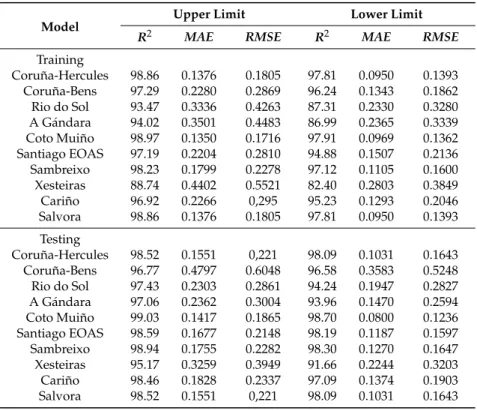
Results show that the models presented two different behaviours (Table9): (i) on the one hand, the models for adaptive setpoint temperatures of the upper limit presented acceptable performances in some of the weather stations, withR2in the testing phase greater than 95% in most of the models, and values ofMAEandRMSElower than 0.3 and 0.4, respectively. The worst estimations were when the running mean temperature presented values which were not within the applicability range of EN 15251 for the upper limit (in the case study analysed, values lower than 15◦C). In such cases, the estimation carried out by the model presented an error of 1◦C (see AppendixA). However, given that these cases are when using heating systems is required, the estimation for the upper limit is acceptable; and (ii) on the other hand, the models for the lower limit presented a low adjustment. In this sense, R2_{ranged between 81.60% and 87.45% in the training phase, and between 86.04% and 91.03% in the} testing phase. Like for the upper limit, this was due to the difficulties of estimating both models for the days in that the running mean temperature was not within the applicability range for the lower limit. This aspect, together with the large number of instances (days) with values of static setpoint temperatures (202 days in the training dataset and 326 days in the testing dataset) made the obtaining of accurate results something of a challenge (AppendixA). The use of the MLRs with approach 2 was not therefore adequate to estimate the adaptive setpoint temperatures accurately.

3.2.2. MLP

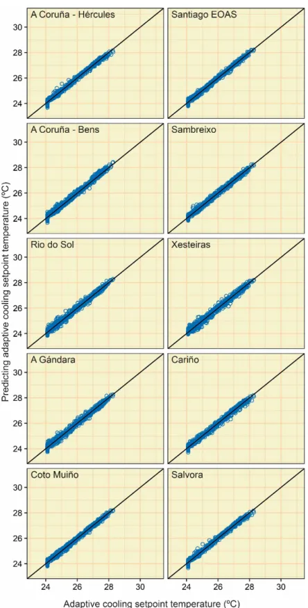
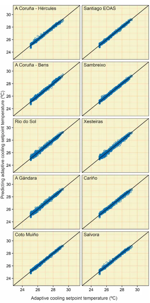
The MLRs of approach 2 did not obtain acceptable results, so the performance that could be obtained with such approach was analysed by using the MLPs as a regression algorithm. Table10 indicates the adequate performance presented by some of the models. Except the weather stations of Coruña-Bens, Rio do Sol, A Gándara, and Xesteiras, the remaining models obtained correlation coefficients greater than 95% in the training and testing phases in both limits, with acceptable error parameters. In this sense, MAEoscillated between 0.0800 and 0.1828, andRMSEbetween 0.1236 and 0.2337 in the estimations of the setpoint temperatures of such models of the upper limit (see FiguresA10–A12) and the lower limit (see FiguresA22–A24). These values allowed estimations to be carried out with an adequate adjustment degree of the adaptive setpoint temperatures of the upper and lower limits.

(16)

Table 9.Results of the training and testing of the MLR models of approach 2.

Model

Table 10.Results of the training and testing of the MLP models of approach 2.

Model

Training Coruña-Hercules 98.86 0.1376 0.1805 97.81 0.0950 0.1393 Coruña-Bens 97.29 0.2280 0.2869 96.24 0.1343 0.1862 Rio do Sol 93.47 0.3336 0.4263 87.31 0.2330 0.3280 A Gándara 94.02 0.3501 0.4483 86.99 0.2365 0.3339 Coto Muiño 98.97 0.1350 0.1716 97.91 0.0969 0.1362 Santiago EOAS 97.19 0.2204 0.2810 94.88 0.1507 0.2136 Sambreixo 98.23 0.1799 0.2278 97.12 0.1105 0.1600 Xesteiras 88.74 0.4402 0.5521 82.40 0.2803 0.3849 Cariño 96.92 0.2266 0,295 95.23 0.1293 0.2046 Salvora 98.86 0.1376 0.1805 97.81 0.0950 0.1393 Testing Coruña-Hercules 98.52 0.1551 0,221 98.09 0.1031 0.1643 Coruña-Bens 96.77 0.4797 0.6048 96.58 0.3583 0.5248 Rio do Sol 97.43 0.2303 0.2861 94.24 0.1947 0.2827 A Gándara 97.06 0.2362 0.3004 93.96 0.1470 0.2594 Coto Muiño 99.03 0.1417 0.1865 98.70 0.0800 0.1236 Santiago EOAS 98.59 0.1677 0.2148 98.19 0.1187 0.1597 Sambreixo 98.94 0.1755 0.2282 98.30 0.1270 0.1647 Xesteiras 95.17 0.3259 0.3949 91.66 0.2244 0.3203 Cariño 98.46 0.1828 0.2337 97.09 0.1374 0.1903 Salvora 98.52 0.1551 0,221 98.09 0.1031 0.1643

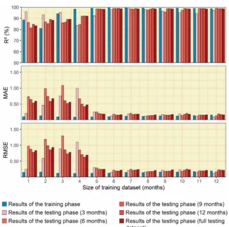
A better estimation obtained by the MLPs was not detected either in those weather stations presenting similar temperature distributions because the correlation coefficients greater than 98% were obtained in the testing phase of the weather stations located in areas with a height difference of more than 200 m, such as Coto Muiñó, Santiago EOAS, and Sambreixo. Given that the MLPs obtained adequate results by using approach 2, the minimum size of the training dataset was analysed as in the models of approach 1. The performances obtained by increasing the number of months included in the

(17)

Energies2019,12, 1197 17 of 47

training dataset are represented in Figure12. As can be seen, the performance of the MLP presented acceptable behaviour when the training dataset included data of 6 months. Such minimum size is the same as that obtained in the MLP of approach 1, so it is shown again the need for having large training datasets to carry out estimations of the adaptive setpoint temperatures accurately.

A better estimation obtained by the MLPs was not detected either in those weather stations presenting similar temperature distributions because the correlation coefficients greater than 98% were obtained in the testing phase of the weather stations located in areas with a height difference of more than 200 m, such as Coto Muiñó, Santiago EOAS, and Sambreixo. Given that the MLPs obtained adequate results by using approach 2, the minimum size of the training dataset was analysed as in the models of approach 1. The performances obtained by increasing the number of months included in the training dataset are represented in Figure 12. As can be seen, the performance of the MLP presented acceptable behaviour when the training dataset included data of 6 months. Such minimum size is the same as that obtained in the MLP of approach 1, so it is shown again the need for having large training datasets to carry out estimations of the adaptive setpoint temperatures accurately.

Figure 12. Influence of the size of the training sample on the MLP model (approach 2).

3.3. Estimation Methodology of the Adaptive Setpoint Temperatures

Based on the results obtained of approaches 1 and 2, the use of MLRs and MLPs allowed the adaptive setpoint temperatures to be accurately estimated. According to the approach used, the regression algorithm presented different behaviour: whereas the MLRs and the MLPs can be used for approach 1, only the use of the MLPs obtained adequate results for approach 2.

The existing differences between the input variables of both approaches imply many possibilities of being used. In this sense, one of such possibilities of using the methods suggested is the configuration of the thermostat of the HVAC system to estimate the setpoint temperature if the external temperature sensor fails (Figure 13). By connecting the thermostat to internet, the data obtained from the weather stations of the meteorological agency of the area (in the present case study, MeteoGalicia) have been imported to generate the data vector to be introduced into the models in order to estimate the adaptive setpoint temperature. Because of possible lacks in the data records (e.g., the setpoint temperature from the previous day has not been recorded or some weather stations fail), the use of both approaches and data from various weather stations (e.g., 5 weather stations) would guarantee the correct estimation of the adaptive setpoint temperatures. If all models can carry out the estimation correctly due to the accuracy obtained in the estimations of the models, the final output value can be obtained by means of the average of the different adaptive setpoint temperatures

Figure 12.Influence of the size of the training sample on the MLP model (approach 2). 3.3. Estimation Methodology of the Adaptive Setpoint Temperatures

Based on the results obtained of approaches 1 and 2, the use of MLRs and MLPs allowed the adaptive setpoint temperatures to be accurately estimated. According to the approach used, the regression algorithm presented different behaviour: whereas the MLRs and the MLPs can be used for approach 1, only the use of the MLPs obtained adequate results for approach 2.

The existing differences between the input variables of both approaches imply many possibilities of being used. In this sense, one of such possibilities of using the methods suggested is the configuration of the thermostat of the HVAC system to estimate the setpoint temperature if the external temperature sensor fails (Figure13). By connecting the thermostat to internet, the data obtained from the weather stations of the meteorological agency of the area (in the present case study, MeteoGalicia) have been imported to generate the data vector to be introduced into the models in order to estimate the adaptive setpoint temperature. Because of possible lacks in the data records (e.g., the setpoint temperature from the previous day has not been recorded or some weather stations fail), the use of both approaches and data from various weather stations (e.g., 5 weather stations) would guarantee the correct estimation of the adaptive setpoint temperatures. If all models can carry out the estimation correctly due to the accuracy obtained in the estimations of the models, the final output value can be obtained by means of the average of the different adaptive setpoint temperatures obtained. This methodology could be used if the external temperature probe fails or in case such probe has been removed because it fails, and another probe cannot be installed. It could also be used if an external temperature probe is provisionally installed in the HVAC system. The probe would be removed when a minimum training size is available to generate the MLRs models of approach 1 (i.e., measurements of 1 month).

(18)

Energies2019,12, 1197 18 of 47 obtained. This methodology could be used if the external temperature probe fails or in case such probe has been removed because it fails, and another probe cannot be installed. It could also be used if an external temperature probe is provisionally installed in the HVAC system. The probe would be removed when a minimum training size is available to generate the MLRs models of approach 1 (i.e., measurements of 1 month).

Figure 13. Estimation methodology of adaptive setpoint temperatures. Failures in the external

temperature probe or temporary installation are considered.

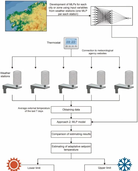
Also, another great possibility to be used is related to approach 2. Unlike approach 1, the MLPs of approach 2 estimated the adaptive setpoint temperatures using only external temperature data. Considering this aspect, configurations of adaptive setpoint temperatures could be implemented in HVAC systems without the need of having external temperature probes, thereby reducing the economic cost of implementing such energy conservation measures, contributing to a high implementation rate, and avoiding possible errors caused by distortions in the measurement of the external temperature during its operation. Therefore, local MLPs could be developed for the different cities or climate zones of a country by using data from weather stations to be used by buildings located in such areas. Like in the methodology shown in Figure 13, the thermostat would be connected to the weather stations of the meteorological agency, and the average values of the external temperature from the previous 7 days would be imported and then introduced into the MLP of each weather station to estimate the adaptive setpoint temperatures (see Figure 14).

Figure 13. Estimation methodology of adaptive setpoint temperatures. Failures in the external temperature probe or temporary installation are considered.

Also, another great possibility to be used is related to approach 2. Unlike approach 1, the MLPs of approach 2 estimated the adaptive setpoint temperatures using only external temperature data. Considering this aspect, configurations of adaptive setpoint temperatures could be implemented in HVAC systems without the need of having external temperature probes, thereby reducing the economic cost of implementing such energy conservation measures, contributing to a high implementation rate, and avoiding possible errors caused by distortions in the measurement of the external temperature during its operation. Therefore, local MLPs could be developed for the different cities or climate zones of a country by using data from weather stations to be used by buildings located in such areas. Like in the methodology shown in Figure13, the thermostat would be connected to the weather stations of the meteorological agency, and the average values of the external temperature from the previous 7 days would be imported and then introduced into the MLP of each weather station to estimate the adaptive setpoint temperatures (see Figure14).

(19)

Energies2019,12, 1197 19 of 47

Figure 14. Estimation methodology of adaptive setpoint temperatures. Not using external

temperature probes is considered. 4. Conclusions

Due to the limitations presented by the implementation of adaptive setpoint temperatures (it should be determined according to the variations of the external temperature), various possibilities of determining such typology of setpoint temperatures without measuring the external temperature are studied in this paper. To achieve this, two approaches were analysed by using two different regression algorithms: a multivariable linear regression and a multilayer perceptron. The approaches were different because of the type of input variables used by each: approach 1 used the setpoint temperature from the previous day and the mean daily external temperature from the previous day, and approach 2 used the mean daily external temperature from the previous 7 days. External temperature data were obtained from 10 weather stations of the meteorological agency MeteoGalicia, which were located at different heights and areas distant from the case study. This allowed the reliability of using the method with data from other climate zones to be ensured.

Based on the results obtained with a dataset of 1040 days, the conclusions are as follows:

• The approach which used the values of setpoint temperature and mean daily external temperature from the previous day to estimate adaptive setpoint temperatures carried out Figure 14.Estimation methodology of adaptive setpoint temperatures. Not using external temperature probes is considered.

4. Conclusions

Due to the limitations presented by the implementation of adaptive setpoint temperatures (it should be determined according to the variations of the external temperature), various possibilities of determining such typology of setpoint temperatures without measuring the external temperature are studied in this paper. To achieve this, two approaches were analysed by using two different regression algorithms: a multivariable linear regression and a multilayer perceptron. The approaches were different because of the type of input variables used by each: approach 1 used the setpoint temperature from the previous day and the mean daily external temperature from the previous day, and approach 2 used the mean daily external temperature from the previous 7 days. External temperature data were obtained from 10 weather stations of the meteorological agency MeteoGalicia, which were located at different heights and areas distant from the case study. This allowed the reliability of using the method with data from other climate zones to be ensured.