Maximum likelihood estimation of a bivariate ordered probit model: implementation and Monte Carlo simulations

Maximum likelihood estimation of a bivariate

ordered probit model: implementation and

Monte Carlo simulations

Zurab Sajaia The World Bank Washington, DC [email protected]

Abstract. We discuss the estimation of a two-equation ordered probit model. We have written a Stata command bioprobitthat computes full-information maxi-mum likelihood estimates of this model. Using Monte Carlo simulations, we com-pare the performance of this and other estimators under various conditions. Keywords: st0001, bivariate ordered probit, maximum likelihood, monte carlo simulations

1

Introduction

The ordered univariate probability models have been applied extensively in biostatics, economics, political science and sociology. Estimations of the joint probability distri-bution of two ordered categorical variables are less common in the literature. The bivariate ordered probit models could be treated as an extension of a standard bivariate probit model when the number of categories of the dependent variables is greater than two. While sharing many properties of bivariate probit estimator, the likelihood func-tion for bivariate ordered probit requires modificafunc-tions in cases when one of underlying DGP contains an endogenous regressor. Despite a potentially wide applicability of this estimator we know of no general routine for estimation of the bivariate ordered prof-itability models, both in seemingly unrelated and simultaneous specifications1_{. In this} paper we describe the implementation of the general full-information maximum (FIML) algorithm to estimate such models. We compare properties of this and other estimators using Monte Carlo simulations.

The econometric problems of estimating a bivariate ordered probability models arise in a variety of settings. For example:

• Calhoun (1989) studies the problem of censoring of desired family size by the num-ber of children ever born. Both models, with and without censoring is effectively seemingly unrelated ordered probit model for two equations.

1. Calhoun (1986) develops a FORTRAN-based routine for the estimation of the seemingly unrelated ordered probit models. Adams (2006) offers a Stata program that implements a FIML algorithm for estimating the SURE bivariate probit models with both dependent variables having three categories

c

• Lawrence and Palmer (2002) examine the connections between attitudes towards a political actor (Hillary Clinton) and an issue that the actor had been actively involved in promoting in studying public opinion about government-run insurance system. The authors estimate seemingly unrelated bivariate ordered probit model for both dependent variables limited to three categories.

• Adams (2006) analyzes the role of R&D spillovers in shaping industrial allocation between learning and internal research. Two dependent variables represent learn-ing shares for academia and industry and are limited to 3 categories. Adams also estimates standard bivariate ordered probit model usingml lf method.

• Scott and Axhausen (2006) use bivariate ordered probit methodology to model the household-level decisions to acquire specific types and numbers of mobility tools. They estimate relationship between number of seasonal tickets and number of cars.

2

Methods

2.1

Model specification

Similar to the univariate ordered probability models, bivariate ordered probability mod-els could be derived from the a latent variable model. Assume that two latent variables y∗₁ andy∗₂ are determined by:

y₁∗_i = x0_1iβ1+ε1i (1)

y₂∗_i = x0_2iβ2+γy1∗i+ε2i (2)

whereβ1andβ2 are vectors of unknown parameters,γ is an unknown scalar,ε1andε2 are the error terms, and subscriptidenotes an individual observation. The explanatory variables in the model satisfy the conditions of exogeneity such thatE(x1iε1i) = 0 and

E(x2iε2i) = 0.

We observe two categorical variablesy1 andy2 such that

y1i=          1 ify₁∗_i≤c11 2 ifc11< y₁∗_i≤c12 .. . J ifc1J−1< y1∗i y2i=          1 if < y∗_2i ≤c21 2 ifc21< y∗_2i≤c22 .. . K ifc2K−1< y∗2i (3)

The unknown cutoffs satisfy the condition thatc11< c12<· · ·< c1J−1andc21< c22<

· · ·< c2K−1. We definec10=c20=−∞andc1J =c2K =∞in order to avoid handling

the boundary cases separately.

The probability thaty1i=j andy2i=kis:

P r(y1i =j, y2i=k) = P r(c1j−1< y1∗i≤c1j, c2k−1< y2∗i≤c2k)

− P r(y₁∗_i≤c1j−1, y2∗i≤c2k)

− P r(y₁∗_i≤c1j, y2∗i≤c2k−1)

+ P r(y1∗i≤c1j−1, y2∗i≤c2k−1) (4)

If εi1 and εi2 are distributed as bivariate standard normal with correlation ρ the individual contribution to the likelihood function could be expressed as:

P r(y1i=j, y2i=k) = Φ2(c1j −x10iβ1, (c2k −γx01iβ1−x 0 2iβ2)ζ, ρ)˜ − Φ2(c1j−1−x01iβ1, (c2k −γx01iβ1−x02iβ2)ζ,ρ)˜ − Φ2(c1j −x01iβ1, (c2k−1−γx01iβ1−x 0 2iβ2)ζ,ρ)˜ + Φ2(c1j−1−x01iβ1, (c2k−1−γx01iβ1−x02iβ2)ζ, ρ)˜ (5) where Φ2is the bivariate standard normal cumulative distribution function,ζ=√ 1

1+2γρ+γ2

and ˜ρ=ζ(γ+ρ). We refer to this specification as simultaneous bivariate ordered probit model. Ifγ = 0 the model simplifies in such a way thatζ = 1 and ˜ρ= ρ. This is a seemingly unrelated specification.

The logarithmic likelihood of an observationiis then

lnLi= J X j=1 K X k=1 I(y1i=j, y2i=k) lnP r(y1i=j, y2i=k) (6)

Under assumptions that observations are independent we can sum (6) across obser-vations to get the log likelihood for the entire sample of sizeN:

lnL= N X i=1 J X j=1 K X k=1 I(y1i =j, y2i=k) lnP r(y1i=j, y2i =k) (7)

2.2

Identification

The parameters in the system of equations (1)-(3) are identified only by imposing an exclusion restriction on vectorsx1 andx2 i.e. at least one element ofx1 should not be present inx2. We cannot use the nonlinearity as a source of identification as it is done in many limited dependent variable setups (e.g. Heckman model) because in the case of exclusion restriction failure, i.e. ifx1=x2, the linear system (1-2) becomes

y₁∗_i = x0_1iβ1+ε1i (8)

y₂∗_i = x0_1i(β2+γβ₁) +ε2i+γε1i (9)

The system 8is unidentified. If we can find some variables that are believed to be correlated with y∗

1 but are independent of theε1, these variables could be included in

3

Monte Carlo simulations

The derivation of the exact asymptotic properties of bivariate ordered probability models with endogenous right-hand side variable could be extremely complicated and perhaps not feasible at all. Even if such formulae would exist they provide no insight about the small sample properties of these estimators. In this section we present an empirical evidence about the behavior of our seemingly unrelated and simultaneous bioprobit

estimator using the Monte Carlo experiments.

3.1

Data-generating process

We generate x1, x2 and z as independent standard normal random variables. Shocks e1 ande2have a correlationρ(we will try different assumptions about the distribution functions). The latent variablesy₁∗ andy₂∗are

y₁∗_i = β10+β11x1i+β12x2i+β13zi+e1i

y₂∗_i = γy∗_1i+β21x1i−β22x2i+e2i (10)

The observed dependent variablesy1 andy2 are defined as:

y1i=            1 if y∗ 1i ≤ −7 2 if −7< y₁∗_i≤ −1 3 if −1< y₁∗_i≤0 4 if 0< y₁∗_i≤3 5 if 3< y₁∗_i y2i=                1 if y∗ 2i≤ −7 2 if −7< y∗ 2i≤ −2 3 if −2< y₂∗_i≤ −1 4 if −1< y₂∗_i≤1 5 if 1< y∗_2i≤2 6 if 2< y∗_2i (11)

We estimate simultaneous specification in both cases of correct and incorrect distribu-tional assumptions about the error terms; then we check efficiency of our SUR estimator. We compare performance of the FIML estimator with three possible alternatives:

• we estimate system (10) with 2SLS;

• we estimate each equation separately using univariate ordered probit method. In case of simultaneity (γ 6= 0), y1 is plugged as an explanatory variable into the equation for y2 in (10)-(11). We refer to these estimates as independent ordered probit (IOP) method in our simulations;

• we apply a ”two-step” procedure, in which we estimate the first equation of system 10 by univariate ordered probit, predicty∗_1i based on the estimated parameters, and use this predicted variable as a regressor in the second univariate ordered probit estimation.

For all simulations, values for the parameters in (10) areβ10 =β11 =β13 =β21 = 1, β12= 2, andβ22=−2. In the simultaneous modelγ= 0.4.

3.2

Simultaneous model with normally distributed error terms

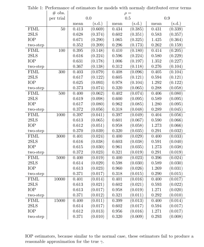
In this simulation, error termse1 and e2 are distributed as bivariate standard normal with correlationρ. We run 1000 replications for each value ofρ={0,0.5,0.9}and for the number of observations ranging from 50 to 15000. We report sample means and sample standard deviations of these 1000 estimates. Table 1 shows the results of simulations for the parameter γ in (10) estimated by FIML and three alternative estimators for different values ofρand different sample size.

For the small samples, the FIML estimator performs well recovering the true param-eterγ = 0.4. However the precision of this estimator is quite low for the sample sizes less than 300 observations. On samples of 3000 observations and more FIML produces unbiased estimates ofγwith small variance. At the same time, the estimates of γ gen-erated by any of the three alternative methods are biased even for the sample sizes of 15000 observations. The bias in estimatingγ increases for higher ρin both, IOP and two-step methods. The 2SLS method also produces biased estimates ofγ but the size of the bias depends neither onρnor on the sample size.

These results are as expected, because both, 2SLS and two-step methods assume (incorrectly) that values of categorical variabley1 approximate those of the latent con-tinuous variabley∗1: in estimating the equation fory∗2in (10) 2SLS usesx1(x01x1)

−1

x01y1

(the predicted value from the first-stage OLS) and IOP method uses justy1, which can-not in general be expected to carry distributional information about the unobserved y∗

1 (except of course, ordering of the categories). While the two-step method comes somehow close in estimating the true value ofγwhenρ= 0, its bias increases when the interaction between two equations in (10) gets stronger whenρ6= 0.

In addition, FIML provides consistent estimate for ρ (not shown here) and also correct standard errors for the parameters; non of the alternative methods do so.

3.3

Simultaneous model: non-normal shocks

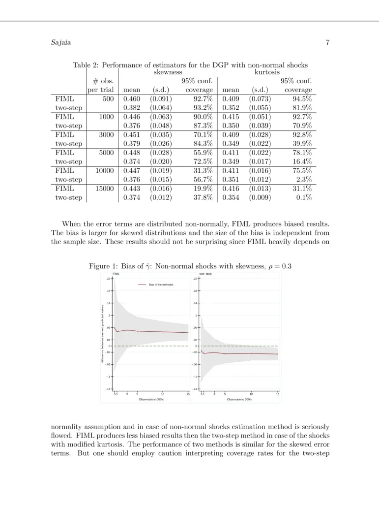
In Table 2 we present the results of M-C simulations for DGP where we modify the errorse1 ande2to be non-normal by altering the skewness and kurtosis.

We apply following transformation to generate the skewness in the errors: e0₁ = χ 2 (5,F(e_{1 ))} √ 10 e0₂ = χ 2 (5_√,F(e2 )) 10 and e0₁ = t(4,F_√(e1 )) 2 e0₂ = t(4,F_√(e2 )) 2 in order to get the kurtosis excess.

Table 1: Performance of estimators for models with normaly distributed error terms

# obs. ρ=

per trial 0.0 0.5 0.9

mean (s.d.) mean (s.d.) mean (s.d.)

FIML 50 0.413 (0.669) 0.434 (0.385) 0.431 (0.339) 2SLS 0.628 (0.374) 0.602 (0.351) 0.583 (0.357) IOP 0.671 (0.290) 1.065 (0.325) 1.425 (0.364) two-step 0.352 (0.209) 0.296 (0.173) 0.262 (0.159) FIML 100 0.395 (0.148) 0.410 (0.180) 0.414 (0.205) 2SLS 0.616 (0.224) 0.596 (0.224) 0.580 (0.229) IOP 0.631 (0.178) 1.006 (0.197) 1.352 (0.227) two-step 0.367 (0.138) 0.312 (0.118) 0.276 (0.104) FIML 300 0.403 (0.079) 0.408 (0.096) 0.405 (0.104) 2SLS 0.617 (0.122) 0.605 (0.121) 0.594 (0.121) IOP 0.625 (0.093) 0.978 (0.104) 1.292 (0.122) two-step 0.373 (0.074) 0.320 (0.065) 0.288 (0.058) FIML 500 0.400 (0.062) 0.402 (0.074) 0.406 (0.080) 2SLS 0.619 (0.098) 0.600 (0.095) 0.589 (0.095) IOP 0.617 (0.080) 0.962 (0.085) 1.280 (0.095) two-step 0.372 (0.056) 0.318 (0.048) 0.289 (0.045) FIML 1000 0.397 (0.041) 0.397 (0.049) 0.404 (0.056) 2SLS 0.613 (0.065) 0.601 (0.067) 0.590 (0.066) IOP 0.612 (0.051) 0.958 (0.058) 1.273 (0.066) two-step 0.370 (0.039) 0.320 (0.035) 0.291 (0.032) FIML 3000 0.401 (0.024) 0.400 (0.029) 0.400 (0.033) 2SLS 0.616 (0.038) 0.603 (0.038) 0.591 (0.040) IOP 0.615 (0.030) 0.961 (0.035) 1.273 (0.038) two-step 0.372 (0.023) 0.321 (0.019) 0.291 (0.019) FIML 5000 0.400 (0.019) 0.400 (0.023) 0.396 (0.024) 2SLS 0.614 (0.029) 0.598 (0.030) 0.589 (0.030) IOP 0.613 (0.023) 0.960 (0.026) 1.269 (0.031) two-step 0.371 (0.017) 0.318 (0.015) 0.290 (0.015) FIML 10000 0.401 (0.014) 0.401 (0.016) 0.400 (0.017) 2SLS 0.613 (0.021) 0.602 (0.021) 0.593 (0.022) IOP 0.613 (0.017) 0.958 (0.019) 1.271 (0.020) two-step 0.371 (0.012) 0.321 (0.011) 0.292 (0.010) FIML 15000 0.400 (0.011) 0.399 (0.013) 0.400 (0.014) 2SLS 0.614 (0.017) 0.602 (0.017) 0.594 (0.017) IOP 0.612 (0.013) 0.956 (0.016) 1.271 (0.017) two-step 0.371 (0.010) 0.320 (0.009) 0.293 (0.008)

IOP estimators, because similar to the normal case, these estimators fail to produce a reasonable approximation for the trueγ.

Table 2: Performance of estimators for the DGP with non-normal shocks

skewness kurtosis

# obs. 95% conf. 95% conf.

per trial mean (s.d.) coverage mean (s.d.) coverage

FIML 500 0.460 (0.091) 92.7% 0.409 (0.073) 94.5% two-step 0.382 (0.064) 93.2% 0.352 (0.055) 81.9% FIML 1000 0.446 (0.063) 90.0% 0.415 (0.051) 92.7% two-step 0.376 (0.048) 87.3% 0.350 (0.039) 70.9% FIML 3000 0.451 (0.035) 70.1% 0.409 (0.028) 92.8% two-step 0.379 (0.026) 84.3% 0.349 (0.022) 39.9% FIML 5000 0.448 (0.028) 55.9% 0.411 (0.022) 78.1% two-step 0.374 (0.020) 72.5% 0.349 (0.017) 16.4% FIML 10000 0.447 (0.019) 31.3% 0.411 (0.016) 75.5% two-step 0.376 (0.015) 56.7% 0.351 (0.012) 2.3% FIML 15000 0.443 (0.016) 19.9% 0.416 (0.013) 31.1% two-step 0.374 (0.012) 37.8% 0.354 (0.009) 0.1%

When the error terms are distributed non-normally, FIML produces biased results. The bias is larger for skewed distributions and the size of the bias is independent from the sample size. These results should not be surprising since FIML heavily depends on

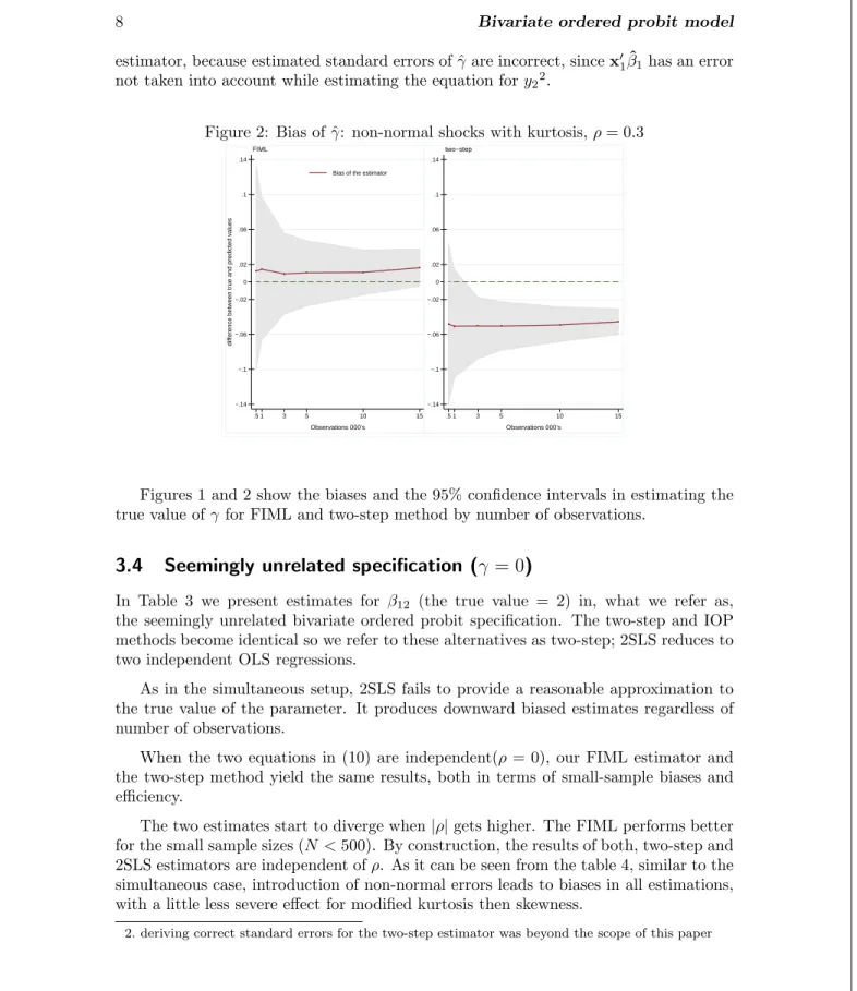
Figure 1: Bias of ˆγ: Non-normal shocks with skewness,ρ= 0.3

−.14 −.1 −.06 −.02 .02 .06 .1 .14 .18 .22 0

difference between true and predicted values

.5 1 3 5 10 15

Observations 000’s Bias of the estimator

FIML −.14 −.1 −.06 −.02 .02 .06 .1 .14 .18 .22 0 .5 1 3 5 10 15 Observations 000’s two−step

normality assumption and in case of non-normal shocks estimation method is seriously flowed. FIML produces less biased results then the two-step method in case of the shocks with modified kurtosis. The performance of two methods is similar for the skewed error terms. But one should employ caution interpreting coverage rates for the two-step

estimator, because estimated standard errors of ˆγare incorrect, sincex0₁β1ˆ has an error not taken into account while estimating the equation fory22.

Figure 2: Bias of ˆγ: non-normal shocks with kurtosis,ρ= 0.3

−.14 −.1 −.06 −.02 .02 .06 .1 .14 0

difference between true and predicted values

.5 1 3 5 10 15

Observations 000’s Bias of the estimator

FIML −.14 −.1 −.06 −.02 .02 .06 .1 .14 0 .5 1 3 5 10 15 Observations 000’s two−step

Figures 1 and 2 show the biases and the 95% confidence intervals in estimating the true value ofγfor FIML and two-step method by number of observations.

3.4

Seemingly unrelated specification (

γ

= 0

)

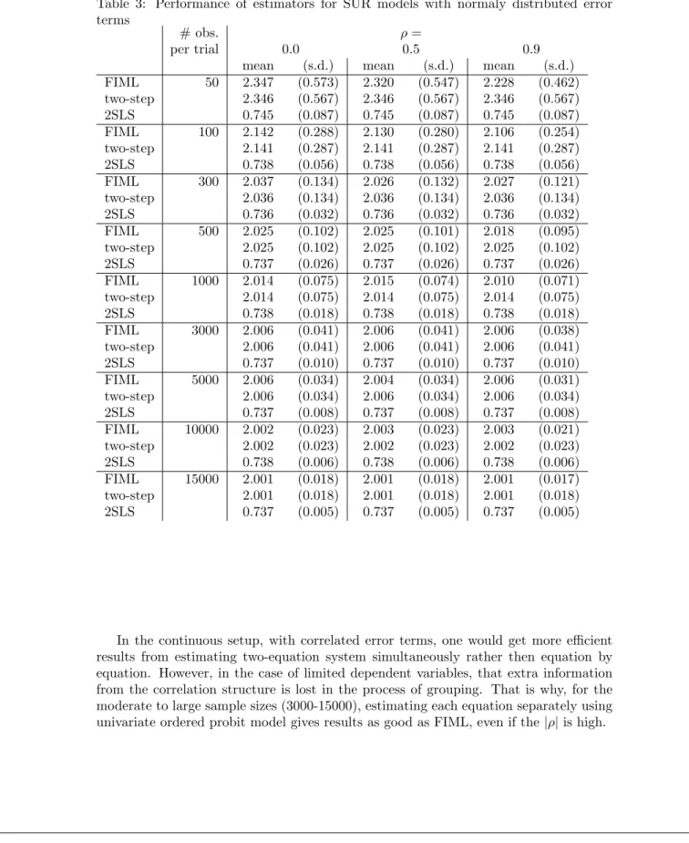
In Table 3 we present estimates for β12 (the true value = 2) in, what we refer as, the seemingly unrelated bivariate ordered probit specification. The two-step and IOP methods become identical so we refer to these alternatives as two-step; 2SLS reduces to two independent OLS regressions.

As in the simultaneous setup, 2SLS fails to provide a reasonable approximation to the true value of the parameter. It produces downward biased estimates regardless of number of observations.

When the two equations in (10) are independent(ρ= 0), our FIML estimator and the two-step method yield the same results, both in terms of small-sample biases and efficiency.

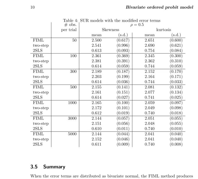
The two estimates start to diverge when|ρ|gets higher. The FIML performs better for the small sample sizes (N <500). By construction, the results of both, two-step and 2SLS estimators are independent ofρ. As it can be seen from the table 4, similar to the simultaneous case, introduction of non-normal errors leads to biases in all estimations, with a little less severe effect for modified kurtosis then skewness.

Table 3: Performance of estimators for SUR models with normaly distributed error terms

# obs. ρ=

per trial 0.0 0.5 0.9

mean (s.d.) mean (s.d.) mean (s.d.)

FIML 50 2.347 (0.573) 2.320 (0.547) 2.228 (0.462) two-step 2.346 (0.567) 2.346 (0.567) 2.346 (0.567) 2SLS 0.745 (0.087) 0.745 (0.087) 0.745 (0.087) FIML 100 2.142 (0.288) 2.130 (0.280) 2.106 (0.254) two-step 2.141 (0.287) 2.141 (0.287) 2.141 (0.287) 2SLS 0.738 (0.056) 0.738 (0.056) 0.738 (0.056) FIML 300 2.037 (0.134) 2.026 (0.132) 2.027 (0.121) two-step 2.036 (0.134) 2.036 (0.134) 2.036 (0.134) 2SLS 0.736 (0.032) 0.736 (0.032) 0.736 (0.032) FIML 500 2.025 (0.102) 2.025 (0.101) 2.018 (0.095) two-step 2.025 (0.102) 2.025 (0.102) 2.025 (0.102) 2SLS 0.737 (0.026) 0.737 (0.026) 0.737 (0.026) FIML 1000 2.014 (0.075) 2.015 (0.074) 2.010 (0.071) two-step 2.014 (0.075) 2.014 (0.075) 2.014 (0.075) 2SLS 0.738 (0.018) 0.738 (0.018) 0.738 (0.018) FIML 3000 2.006 (0.041) 2.006 (0.041) 2.006 (0.038) two-step 2.006 (0.041) 2.006 (0.041) 2.006 (0.041) 2SLS 0.737 (0.010) 0.737 (0.010) 0.737 (0.010) FIML 5000 2.006 (0.034) 2.004 (0.034) 2.006 (0.031) two-step 2.006 (0.034) 2.006 (0.034) 2.006 (0.034) 2SLS 0.737 (0.008) 0.737 (0.008) 0.737 (0.008) FIML 10000 2.002 (0.023) 2.003 (0.023) 2.003 (0.021) two-step 2.002 (0.023) 2.002 (0.023) 2.002 (0.023) 2SLS 0.738 (0.006) 0.738 (0.006) 0.738 (0.006) FIML 15000 2.001 (0.018) 2.001 (0.018) 2.001 (0.017) two-step 2.001 (0.018) 2.001 (0.018) 2.001 (0.018) 2SLS 0.737 (0.005) 0.737 (0.005) 0.737 (0.005)

In the continuous setup, with correlated error terms, one would get more efficient results from estimating two-equation system simultaneously rather then equation by equation. However, in the case of limited dependent variables, that extra information from the correlation structure is lost in the process of grouping. That is why, for the moderate to large sample sizes (3000-15000), estimating each equation separately using univariate ordered probit model gives results as good as FIML, even if the|ρ|is high.

Table 4: SUR models with the modified error terms

# obs. ρ= 0.5

per trial Skewness kurtosis

mean (s.d.) mean (s.d.) FIML 50 2.500 (0.617) 2.651 (0.600) two-step 2.541 (0.996) 2.690 (0.621) 2SLS 0.613 (0.093) 0.754 (0.084) FIML 100 2.361 (0.369) 2.345 (0.300) two-step 2.381 (0.391) 2.362 (0.310) 2SLS 0.614 (0.059) 0.744 (0.059) FIML 300 2.189 (0.187) 2.152 (0.170) two-step 2.203 (0.199) 2.164 (0.171) 2SLS 0.614 (0.036) 0.744 (0.033) FIML 500 2.155 (0.141) 2.081 (0.132) two-step 2.161 (0.151) 2.077 (0.134) 2SLS 0.614 (0.027) 0.741 (0.025) FIML 1000 2.165 (0.100) 2.059 (0.097) two-step 2.172 (0.101) 2.049 (0.098) 2SLS 0.612 (0.019) 0.740 (0.018) FIML 3000 2.144 (0.057) 2.051 (0.055) two-step 2.151 (0.056) 2.048 (0.055) 2SLS 0.610 (0.011) 0.740 (0.010) FIML 5000 2.144 (0.044) 2.041 (0.040) two-step 2.152 (0.046) 2.041 (0.040) 2SLS 0.611 (0.009) 0.740 (0.008)

3.5

Summary

When the error terms are distributed as bivariate normal, the FIML method produces unbiased and more efficient estimates compared to the three alternative estimators. The advantage of the FIML is more visible for simultaneous models (γ 6= 0) or when

|ρ| is high. The FIML estimates are biased when the shocks are not normal. The bias persists even in the large samples. The two-step estimator performs better with the distribution of the error terms is skewed. In the seemingly unrelated setup (γ = 0), the FIML estimator demonstrates no efficiency gains relative to two-step method. It however, performs better on the small samples and especially for higher values of|ρ|. The FIML estimator is the only method that estimate the value ofρ.

4

Algorithm Implementation

A full-information maximum-likelihood estimation of the model is implemented as anml d2evaluator that computes the log likelihood for each observation, along with its

analyt-ical gradient and Hessian matrix3_{. To make sure that estimatedρsatisfies−1≤ρ≤1} and cutoffs are ordered ascending we transform the parameters before passing them to

ml. We estimate arctanh(ρ) in place of ρ, and (c11,√c12−c11, . . . , √c1J−1−c1J−2)

and (c21,√c22−c21, . . . ,√c2K−1−c2K−2) in place of (c11, . . . , c1J−1) (c21, . . . , c2K−1)

respectively. Results are displayed for the original parameters.

The initial values passed to ml are obtained by estimating independent ordered probit model for each equation.

5

The

bioprobit

command

5.1

Syntax

The bioprobit command fits maximum-likelihood two equation ordered probit models either in seemingly unrelated or in simultaneous specifications.

bioprobit depvar1 depvar2 varlist

if

in

weight

, offset1(varname) offset2(varname) collinear robust cluster(varname) level(#)

maximize options Or bioprobit (depvar1 = varlist1) (depvar2 = varlist2) if in weight , endogenous offset1(varname) offset2(varname) collinear robust cluster(varname) level(#) maximize options

fweights,pweights, andiweights are allowed.

5.2

Options

endogenousspecifies that the model to be estimated is simultaneous (γ6= 0). If avail-able, instrument(s) should be included invarlist1.

offset1(varname1) offset2(varname2)specify thatvarname1 and/or varname2 be included in the model with the coefficient constrained to be 1.

robustcomputes robust estimates of variance.

cluster(varname)adjusts standard errors for intragroup correlation.

level(#)sets the level for confidence intervals, in percent. The default islevel(95)

or as set byset level.

maximize optionsare passed directly tomland control the maximization process.

5.3

Postestimation

The following statistics are available for thepredictpostestimation command:

outcome(j, k) or outcome(#j, #k) computes the predicted probability P r(y1i =

j, y2i = k) or P r(y1i = y1j, y2i = y2k). If one of the arguments is missing then result will be the marginal probability, i.e. outcome(., k) will return P r(y2i =

k) =PJ

j=1P r(y1i=j, y2i=k).

xb1calculatesx0_1iβˆ1.

xb2calculatesx0_2iβ2.ˆ

stdp1 calculates the standard error of the linear prediction of equation 1.

stdp2 calculates the standard error of the linear prediction of equation 2.

6

Example

We illustrate the use of thebioprobitcommand by estimating the economic gradient in self-assessed health status on the survey data for Russia (Lokshin and Ravallion (2005)). The economic model postulates the bivariate relationship between individual’s health status and economic welfare. Neither characteristic is directly observable. Respondents report the categories of the subjective assessment of their health and wealth status.

The underlying model consists of two equation relating the latent health (H) and wealth (W) status to individual characteristics of the respondents x:

Wi = x01iβ1+ε1i (12)

Hi = γWi+x02iβ2+ε2i (13)

The observed variables for the individual’s subjective health (SAH) and subjective wealth (SAW) assessments are related to the corresponding latent variables as:

SAHi=            1 - very bad if Hi≤µ1 2 - bad ifµ1< Hi≤µ2 3 - average ifµ2< Hi≤µ3 4 - good ifµ3< Hi≤µ4 5 - very good ifµ4< Hi SAWi=          1 - poor if Wi≤δ1 2 ifδ1< Wi≤δ2 .. . 7 - rich ifδ6< Wi

Assuming that ε1 and ε2 are distributed normally N(0,P

) the system could be estimated by FIML implemented inbioprobit. The system (12)-(13) is identified by non-linearity (although weakly), but we introduce an instrument in equation (12) to improve identification properties of the model. As an instrument we the logarithm of per-capita consumption of households averaged across their particular locality of residence, The paper argues that this variable while directly affecting the subjective wealth perception has no direct effect on the subjective assessment of health.

. bioprobit (econrnk ‘ostr’ mean_logexp) (sr_health ‘ostr’) , end initial: log likelihood = -26616.3

rescale: log likelihood = -26616.3 rescale eq: log likelihood = -23689.019

Iteration 0: log likelihood = -23689.019 (not concave) Iteration 1: log likelihood = -23608.069 (not concave) Iteration 2: log likelihood = -23606.768

(output omitted)

Iteration 12: log likelihood = -23598.033

Simultaneous bivariate ordered probit regression Number of obs = 9049 Wald chi2(23) = 965.64 Log likelihood = -23598.033 Prob > chi2 = 0.0000 Coef. Std. Err. z P>|z| [95% Conf. Interval] econrnk exp_ppl .1234239 .007774 15.88 0.000 .1081872 .1386605 exp_2 -.4390104 .0373828 -11.74 0.000 -.5122794 -.3657414 exp_3 .0323373 .0033307 9.71 0.000 .0258092 .0388654 ind_nincm .2210446 .0339821 6.50 0.000 .1544409 .2876482 hhsize .0572405 .0082824 6.91 0.000 .0410074 .0734736 sskids -.0121174 .1149387 -0.11 0.916 -.2373932 .2131583 sbkids .082298 .0823023 1.00 0.317 -.0790115 .2436076 spens -.0664515 .0622542 -1.07 0.286 -.1884674 .0555644 sawomen .2369426 .0752543 3.15 0.002 .0894469 .3844382 age -.0507569 .0041248 -12.31 0.000 -.0588414 -.0426725 age2 .0476939 .0043854 10.88 0.000 .0390987 .056289 educat_2 .1107387 .0585926 1.89 0.059 -.0041007 .2255782 educat_3 .055761 .0662793 0.84 0.400 -.0741441 .1856661 educat_4 .1900912 .052825 3.60 0.000 .0865561 .2936264 educat_5 .1917961 .0537008 3.57 0.000 .0865444 .2970478 educat_6 .1812265 .0556275 3.26 0.001 .0721987 .2902544 married .1790618 .0418981 4.27 0.000 .096943 .2611805 divorced -.0952741 .0547488 -1.74 0.082 -.2025798 .0120317 ltogether -.0270486 .0495721 -0.55 0.585 -.1242081 .0701108 widowed -.0744711 .0560572 -1.33 0.184 -.1843412 .0353991 hasjob -.0076203 .0315105 -0.24 0.809 -.0693797 .054139 unem_b -.1803119 .0584877 -3.08 0.002 -.2949458 -.0656781 mean_logexp -.1892784 .0428467 -4.42 0.000 -.2732564 -.1053005 sr_health exp_ppl -.0935869 .0134526 -6.96 0.000 -.1199534 -.0672203 exp_2 .3525307 .053468 6.59 0.000 .2477353 .457326 exp_3 -.02647 .0043955 -6.02 0.000 -.035085 -.0178551 ind_nincm -.1202432 .0442456 -2.72 0.007 -.2069631 -.0335234 hhsize -.0060836 .0154725 -0.39 0.694 -.0364092 .0242421 sskids .0650188 .121711 0.53 0.593 -.1735304 .303568 sbkids -.1308044 .0868541 -1.51 0.132 -.3010352 .0394265 spens .0574917 .0655659 0.88 0.381 -.0710151 .1859985 sawomen -.3625286 .0796968 -4.55 0.000 -.5187315 -.2063257 age .023076 .0089286 2.58 0.010 .0055763 .0405758 age2 -.042675 .0057854 -7.38 0.000 -.0540142 -.0313358 educat_2 .0695105 .0705092 0.99 0.324 -.0686849 .207706 educat_3 .1054092 .0746369 1.41 0.158 -.0408764 .2516948 educat_4 .0525468 .0736925 0.71 0.476 -.0918878 .1969815 educat_5 .0663105 .0760016 0.87 0.383 -.0826499 .2152709 educat_6 .1217773 .0817214 1.49 0.136 -.0383937 .2819483 married -.1797039 .0458573 -3.92 0.000 -.2695826 -.0898251 divorced -.0243082 .0639908 -0.38 0.704 -.1497277 .1011114

ltogether -.064558 .0546643 -1.18 0.238 -.1716981 .0425821 widowed -.0227709 .0624224 -0.36 0.715 -.1451166 .0995747 hasjob .1469339 .0405737 3.62 0.000 .067411 .2264569 unem_b .2628048 .0616775 4.26 0.000 .1419191 .3836906 athrho _cons -.9656639 .2386267 -4.05 0.000 -1.433364 -.4979641 gamma _cons .8369609 .0895959 9.34 0.000 .6613562 1.012566 /cut11 -2.159789 .1102107 -2.375798 -1.94378 /cut12 -1.455243 .1091092 -1.669093 -1.241393 /cut13 -.6745846 .1086014 -.8874394 -.4617297 /cut14 .0163376 .1084458 -.1962124 .2288875 /cut15 .8873047 .108811 .674039 1.10057 /cut16 1.335976 .1097295 1.12091 1.551041 /cut21 -2.328086 .4103713 -3.132399 -1.523773 /cut22 -1.507293 .2684242 -2.033395 -.9811915 /cut23 -.1557551 .0810297 -.3145705 .0030603 /cut24 1.061703 .2169265 .6365349 1.486871 rho -.7467926 .1055448 -.8923539 -.4605145 LR test of indep. eqns. : chi2(1) = 145.02 Prob > chi2 = 0.0000

The Likelihood Ratio or Wald test can be performed to test the independence of equa-tions hypothesis (ρ= 0). By default, results of LR test are shown, but if eitherclaster

option or pweight was used, the Wald test that ρ = 0 will be reported. In case of SUR model, the alternative specification is to fit an univariate ordered probit model for each equation. For the simultaneous ordered probit model, the two-step estimator used above serves as an alternative. For our example, the null hypothesis is strongly rejected.

After estimating the model, we can get predicted probabilities for any combination of states. Lets calculate what is the predicted marginal probability of that average person in our sample reports his or her health as very bad (SAHi = 5), and by how much

this probability would change if percapita incomes and expenditures were to increase by 10%.

. predict p1, outcome(., #1) . summarize p1

Variable Obs Mean Std. Dev. Min Max p1 9061 .0277679 .0519662 .0000298 .4838202 . local p1=r(mean)

. replace exp_ppl_11=exp_ppl_11*1.1 (9126 real changes made)

. replace exp_2=exp_2*(1.1)^2 (9126 real changes made)

. replace exp_3=exp_3*(1.1)^3 (9126 real changes made)

. replace ind_nincm=ind_nincm*1.1 (9273 real changes made)

. predict p2, outcome(.,#1) . summarize p2

Variable Obs Mean Std. Dev. Min Max p2 9061 .0275784 .0517408 .0000184 .4818855 . display (r(mean)/‘p1’-1)*100

-.68244268

The average effect of 10% increase in percapita incomes and expenditures would be the 0.7% reduction in predicted marginal probability of having bad health.

7

References

Adams, J. D. 2006. Learning, Internal Research, and Spillovers.Economics of Innovation

and New Technology 15(January): 5–36.

Calhoun, C. 1986. BIVOPROB: Maximum Likelihood Program for Bivariate Ordered-Probit Regression. The Urban Institute .

———. 1989. Estimating the Distribution of Desired Family Size and Excess Fertility.

The Journal of Human Resources 24(4): 709–724.

Lawrence, C. N., and H. D. Palmer. 2002. Heuristics, Hillary Clinton, and Health Care Reform. Annual Meeting of the Midwest Political Science Association.

Lokshin, M., and M. Ravallion. 2005. Searching for the economic gradient in self-assessed health. Policy Research Working Paper 3698.

Scott, D. M., and K. W. Axhausen. 2006. Household mobility tool ownership: modeling interactions between cars and season tickets. Transportation from Springer 33(4): 311–328.

About the authors

Zurab Sajaia works in the Development Economics Research Group of the World Bank.

Appendix

Here we derive analytical first and second derivatives of the likelihood function. As described in section 4, we define additional parameters:r=arctanh(ρ);d11=c11, d12=

√ c12−c11, . . . , d1J−1= √ c1J−1−c1J−2) andd21=c21, d22= √ c22−c21, . . . , d2K−1=

√

c2K−1−c2K−2). Therefore, complete set of parameters we estimate is

Θ≡ {β1, β2, γ, r, d11, . . . , d1J−1, d21, . . . , d2K−1}

First Derivatives

Then first derivative with respect to parameter θ∈Θ is ∂lnL ∂θ = 1 L ∂Φ2(A11, A21, ρ0) ∂θ − ∂Φ2(A12, A22, ρ0) ∂θ − ∂Φ2(A13, A23, ρ0) ∂θ + ∂Φ2(A14, A24, ρ0) ∂θ

lets introduce some more notation:

A11=A13 = c1j −β10x1i A12=A14 = c1j−1−β10x1i A21=A22 = ζ(c2k −γβ10x1i−β02x2i) A23=A24 = ζ(c2k−1−γβ10x1i−β20x2i) Φs_≡Φ 2(A1s, A2s,ρ) for˜ s= 1. . .4

First partial derivatives of the bivariate standard normal CDF are:

Φs1 = φ(A1s)F A2s−ρA˜ 1s p 1−ρ˜2 ! Φs₂ = φ(A2s)F A1s−ρA˜ 2s p 1−ρ˜2 ! Φs3 = 1 2πp1−ρ˜2exp −1 2 _A2 1s+A22s−2 ˜ρA1s A2s 1−ρ˜2

Then derivatives ofA1s,A2s and ˜ρwith respect to each parameter are:

∂A1s ∂β1 = −1 ∂A1s ∂d11 = 1 ∂A1s ∂d1j = 2d1j ∂A2s ∂β1 = −ζγ ∂A2s ∂β2 = −ζ ∂A2s ∂r = −A2sζ 2_γdρ dr

∂A2s ∂γ = −A2sζρ˜−ζβ1 ∂A2s ∂d21 = ζ ∂A2s ∂d2k = 2ζd2k ∂ρ˜ ∂r = ζ(1−ζγρ)˜ dρ dr ∂ρ˜ ∂γ = ζ(1−ρ˜ 2₎ dρ dr = 4 exp2r (1 + exp2r₎2

Second Derivatives

∂2lnL ∂θ1∂θ2 = L −1 ∂ 2_L ∂θ1∂θ2 −L −2∂L ∂θ1 ∂L ∂θ2 ∂2L ∂θ1∂θ2 = ∂2Φ1 ∂θ1∂θ2− ∂2Φ2 ∂θ1∂θ2 − ∂2Φ3 ∂θ1∂θ2 + ∂2Φ4 ∂θ1∂θ2 ∂2_Φ ∂θ1∂θ2 = 3 X ij=1 Φsij ∂Ais ∂θ1 ∂Ajs ∂θ2 + Φ s 1 ∂2_A 1s ∂θ1∂θ2+ Φ s 2 ∂2_A 2s ∂θ1∂θ2 + Φ s 3 ∂2_A 3s ∂θ1∂θ2 where we used notationA3s≡ρ0.

Second partial derivatives of the bivariate standard normal CDF are:

Φs₁₁ = −A1sΦs1−ρΦ˜ s 3 Φs₁₂ = Φs₃ Φs₁₃ = Φs₃ρA2˜ s−A1s 1−ρ˜2 Φs₂₂ = −A2sΦs2−ρΦ˜ s 3 Φs₂₃ = Φs₃ρA1˜ s−A2s 1−ρ˜2 Φs₃₃ = Φs₃A1sA2s+ρ 0_−ρ˜A2_1s+A2_2s−2 ˜ρA1sA2s 1−ρ˜2 1−ρ˜2 ∂2_A 1s ∂d2 1j = 2

∂2_A2 s ∂β1∂r = ζ3γ2dρ dr ∂2_A 2s ∂β1∂γ = ζ 2 γρ˜−ζ ∂2_A2 s ∂β2∂r = ζ3γdρ dr ∂2_A 2s ∂β2∂γ = ζ 2_ρ˜ ∂2_A2 s ∂r2 = 3A2sζ 4_γ2 _dρ dr 2 −A2sζ2γ d2_ρ dr2 ∂2A2s ∂r∂γ = −3A2sζ 2_{(1 ˜ρ}2_{) +β1ζ}3_γdρ dr ∂2_A2 s ∂r∂d21 = −ζ3γdρ dr ∂2A2s ∂r∂d2k = −2d2kζ3γ dρ dr ∂2_A 2s ∂γ2 = A2s(3ζ 3_γρ˜−ζ2_{) + 2β1ζ}2_ρ˜ ∂2_A2 s ∂γ∂d21 = −ζ2ρ˜ ∂2_A 2s ∂γ∂d2k = −2d2kζ2ρ˜ ∂2A2s ∂d2 2k = 2