Determinants of the Levels of Development Based on the Human Development Index:Bayesian Ordered Probit Model

Issues

ISSN: 2146-4138

available at http: www.econjournals.com

International Journal of Economics and Financial Issues, 2017, 7(5), 425-431.

Determinants of the Levels of Development Based on the Human

Development Index: Bayesian Ordered Probit Model

Ebru Çağlayan-Akay

_{, M. Hanifi Van}

_*

1_{Department of Econometrics, Marmara University, Istanbul, Turkey,} 2_{Department of Econometrics, Yüzüncü Yıl University, Van,} Turkey. *Email: [email protected]

ABSTRACT

The aim of the paper is to determine the factors affecting the economic development levels of selected countries using bayesian ordered probit model.

For this aim, human development ındices of 130 countries are involved in the analysis with respect to seven independent variables for the period of 2009-2014. According to the results obtained from the Bayesian ordered probit model, it was observed that while the variables of rural population,

health expenditure, gross domestic product (GDP), internet users, life expectancy at birth, share of expected years of schooling seats in parliament had a positive effect on human development level in short term; the variables of health expenditure, GDP, internet users, share of expected years of schooling and seats in parliament had a positive effect,butrural population and life expectancy at birth had a negativeimpact on human development in long term.

Keywords: Human Development Indices, Ordered Probit, Bayesyen, Economic Development

JEL Classifications: O150, C250, C110, O100

# _{This study is derived from a dissertation.}

1. INTRODUCT

I

ON

The Human Development Report, first published in 1990, has brought a new approach for the development of human welfare, unlike economic development. Human development, or human progress approach draws attention to the richness of human life rather than the richness of human prosperity.One of the most important achievements of the human progress approach is to provide gradually acceptance of the reality that monetary measures such as gross domestic product (GDP) per capita are inadequate tools in the indication of human progress. The first human development report introduced human development ındex (HDI) as a success criterion in the basic dimensions of human development between countries. Every year, human development report reviews where the countries stand in respect to HDI using four categories including very high human development, high human development, moderate human development, and low human development (Portnoi, 2016). In other words, progress is associated with the increase of the options in the direction of which, people will live a desired lifestyle (United Nations Development Programe, hereafter [UNDP], 2016b). HDI, prepared

by UNDP, compares the progress, measured with the indications including more educated individuals, long life expectancy and high income, with the progress in human development in general.

HDI has been constituted to emphasize that people and their skills should be the ultimate criteria for the assessment of the development of an country, not just for that of economic growth. HDI is an index that discusses and measures long-term progress within the scope of three basic dimensions of human development including “a long and healthy life,” “access to information,” “decent living conditions.”

The commence of HDI application arousedanextensive interest by reflecting conventionalGDP percapita or general dissatisfaction of real wages, asbeing a measure ofthe changes in living standards. HDI has been conceived as a development including prosperity and quality of life, going beyond special revenues and purchasing power Hou et al. (2015). However, there are basically three criticisms of the human development index. First one, it neglects a few different dimensions of human health, such as human rights, security and political participation (Anand and Sen, 2000). The second one, it only takes average achievements into account, and therefore, it does not consider the distribution of human development in a country (Sagar and Najam, 1998). The last one, a wider group of government actors and civil society actors are not included in the decision-making process (Sharma and Sharma (2015).

The aim of the study is to examine the factors affecting the levels of development of 130 countries selected for 2009-2014 period. For this aim, Bayesian ordered probit model, an aproach that has recently come into use, was used. The reason for using this model is to review both the short-term and long-term effects of the factors affecting the level of human development, and to determine whether these effects change over time.

This study differs from the previous studies in two respects. The first one, it deals with countries with different levels of development. The studies conducted on human development have generally focused on a limited number of countries with very high development and high development levels. 130 countries with moderate, high and very high levels of development were reviewed in this study. Secondly, both short-term and long-term effects of the variables reviewed can be examined through the method used. Thus, necessary information can be obtained regarding to which factors should be attached importance by the countries with moderate and high levels of development in order to reach a very high level of development in short and long term.

The paper is organized as follows: Section 2 reviews the existing literature to exhibit the studies that concentrate on the evaluation of the HDI data using several econometric methods. Section 3 gives general information about the theoretical background of bayesian ordered probit model. Section 4 introduces the methodology of the study and the data being used to perform the analysis. Section 5 presents the results of the bayesian ordered probit estimation and the interpretation of the underlying results in detail. Conclusions are given in Section 5.

2. L

I

TERATURE REV

I

EW

HDI report was published by UNDP in 1990 for the first time. There are many studies in the literature, conducted in order to investigate the living conditions of countries. Lee et al. (2006) reviewed the HDI by data envelopment analysis, and evaluated the relative performance of countries through a model based on fuzzy multiple objective, and using the best common weights for HDI component indices.

Blanchflower and Oswald (2005) brought the questions forward about Australia’s rank as number three in world ranking according

to HDI value. They reviewed new studies conducted on happiness economy, and evaluated the results for policy makers. They showed by using new ISSP data of about 50,000 randomly selected individuals from 35 countries that Australia’s job satisfaction level is nearly below of the average ofan international ranking.

Davies and Quinlivan (2006) assessed the existence ofa positive correlationbetween the developments at the level of social welfare and increasingtrade, within the scope ofa multinational multi-year panel data analysis. By using the generalized method of moments (GMM) procedure in the panel data framework, they found that the increase in trade is positively related with the social welfare increase in the future.

Grimm et al. (2008) revealed with a new methodology that how three-dimensional index would be calculated with common data sources for society categories withdifferent distribution of income. They compared the level of development of people in low-income group, with the level of domestic and foreignpeople with high - income.

Johnson (2008) tried to explain that to what extent GDP and HDI, developed by united nations development programme,made contribution to explain subjective happiness. He stated in the article that he hadfoundby using ordered probit model that the countries with high GDP, HDI, and level of income per capita werehappier in general.

Davies (2009) investigated the effect of government consumption expenditures measured by the HDI on social welfare. He offered evidences suggesting that the most appropriate dimension of government according to human development measures is clearly higher than that according to GDP measures,by using dynamic GMM estimation in the panel data frame, in the context of multi-country and multi-year panel data analysis.

Abayomi and Pizarro (2013) presented a simple framework to measure the progression in many dimensions by using international social indices by which they classified multivariate country-level data as linear combinations of univariate point. They used Bayesian algoritm to generate contingent (confidence-type) intervals for point estimations of country scores.

Eren et al. (2014) investigated the factors affecting countries’ development levels using several regression models for limited dependent variables that contain binary logit, probit and tobit analyses. The results of all regression models showed that the variables, containing life expectancy at birth, share of expected years of schooling, labour force participation rate (female-male ratio) and GDP per capita, have statistically significant effects on the level of development of the countries.

terms of human development, according to human development indicator, regardless of the effect of tourism.

3. BAYES

IA

N D

YNAMIC

LATENT

ORDERED

PROB

I

T MODEL

Panel ordered multiple-choice models are those in which dependent variable takes more than two values, and that there are an ordered composition among these options, and are widely used in the literature. There are too few studies in which Bayesian approach have been recently used for panel ordered models. For example, Bayesian method was used to estimate Hasegawa (2009) dynamic panel-ordered probit model. Four alternative algorithms were compared for estimating ordered probit models. It showed that income and savings have positive effects on life satisfaction, and marital and labor participation rates of posterior results have the same negative effects. Stegmueller (2013) used a Bayesian dynamic panel model that facilitates the analysis of repeated choices by using individual-level panel data. He obtained the model through a robust alternative based on bayesiannon-parametric density estimation. By using this model, and Britannia household panel study conducted from 1991 to 2007, he analyzed the impact of income and wealth on intervention preferences.

The Bayesian approach has some advantages compared to the panel ordered models. The Bayesian approach has very attractive features on frequency statistics. Especially, missing data and latent variables usually do not pose a problem in Bayesian analyses.

The Bayesian approach provides the ability to add prior knowledge to the parameters. The parameters themselves follow a probability distribution in a Bayesian approach, and alsoparameters, model parameters areincomplete data, or (latent) unobserved events (Gelman et al., 2004). The maximum likelihood method (MLE) is used for the estimation of the panel ordered models. The Bayesian estimation method has some advantages compared to the MLE method. Firstly, it eliminates the problem of irregular optimal solutions resulting from different starting points. While the MLE method is critically based on the starting point, the Bayesian estimation method avoids this problem by directly evaluating the probability function (McCulloch and Rossi, 1994). Secondly, the Bayesian estimation method guarantees the consistency and effectiveness of results under more favorable conditions (Byun and Lee, 2017).

A data enhancement method is used to facilitate the implementation of the Bayesian ordered probit model. z latent variables are treated as unknown parameters to be estimated for this data enhancement method, and final common posterior distribution is established for β, γ* and z (Albert and Chib, 1993). The references should be expressedas a latentvariable z_t that represents the basis of continuous concepts that generateobserved categorical scores (Greene and Henster, 2010). When we look from the conceptual perspective of preferences, since there is no reason to expect that the current continuous preferences depend on the preference categories in the past, we also need latent variables to appear on

the right side of our dynamic panel model (Heckman, 1978; Müller and Czado, 2005; Pudney, 2008). In other words, the feedbacks givenfrom the past preferences to current ones come outfrom z t-1, notfrom yt-1. Thus, by following. Albert and Chib (1993); the observed responses of observed variables, y_it (i=1,……, N;t), in the category c (c=1,……, C) are modelled a vector of z_it a continuous basic latent variable and the initial parameter as follows:

y_it=c if z_it ϵ(τ_c-1, τc) (1)

For Z_it, latentpreferences; dynamic model can be written as follows:

z_it=ϕz_it−1+β'x_it+ξ_i+ϵ_it, t=1.,T (2)

Where, ϕ refers to the degree of continuous preferences, that is, to which extent current preferences are dependent on the previous preferences β is a vector of regression parameters for time-varying independent variables and a general matrix of constants. The faults are separated according to the countries, HDI values of countries,unit time; stationary random effect, ξ_i and stochastic distortions ϵ_it.

For identification, the variance of stochastic errors was distributed as it ~ N ( ,0 )

2

 . It was determined as _2

1

= . Making use of ordered probit specification. Unobserved individual heterogeneity is modeled through random effects obtained from a normal distribution with estimated variance 2 zero mean (Stegmueller, 2013):

it ~ N ( ,0 )

2

 ₍₃₎

The presence of random effects may in time lead to correlations between the responses of the same individuals (Rabe-Hesketh and Skrondal, 2008). After the preference constant is calculated, it is estimated by the individual random effects- related total variance rate ρ σ

σ

ξ

ξ

= +

2

2

1 This provides a useful indicator with regard to the relationship of unobserved individual differences that are ignored and can not be observed in horizontal section analyzes (Stegmuller, 2013). The model specification is completed by distributing priors to all parameters. The following priors, determined by Stegmuller (2013), were used. For intersections and parameters of individual qualities, priors distribute with zero mean and large variance β,δ ~ N(0,100)in dynamic and initial conditional equations to make use of regression-type estimates. They distribute with very large variance ϕ ~ N(0.5,100) İn order to make use of diffuse priors. For random effect random effect, They distribute with non-informative prior zero centered normal distribution and large variance λ ~ N(0,100) .

4. DATA

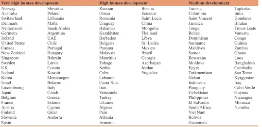
not yet developed, study was done for 130 countries with very high, high and medium development levels. The HDI values of countries in the period of 2009 to 2014 were obtained from human development report prepared by UNDP. The HDI values of 130 countries are given in Table 1.

This study was discussed in the scope of “long and healthy life,” “access to knowledge,” “good living standards”, the three main dimensions that may affect the long-term development of countries. Here, the relationship between the observed responses and the latent variable is given as1_;

y

z

z z

t

it

it

it

=

< = = < <

< 

 

 

-1 0

0 0 1

1 2

2

τ

τ τ

τ ₍₄₎

In order to obtain the ordinal nature of the observed preference scores, the initial parameters were constrained so as to increase monotonically;

−∞=τ₀<τ₁=0<τ₂<...<τ_c−1<τ_c=∞ (5)

and to define the model it was assumed that τ₁=0 (assuming that an entire constant will be included in the model) (Albert and Chib, 1993; Johnson and Albert, 1999).

The factors affecting the developmental level of the 130 countries discussed were examined by using bayesian panel data, as distinct

1 Since there was not a statistical test supporting the reduction of the category number of the likert-scale dependent variable in the study done by Franses

and Cramer (2010), the dependent variable was shown in this way by

Stegmuller (2013).

from the panel ordered probit, and thus, it was aimed to analyze the dynamics of unitary preferences and attitudes. Despite the fact that there are many factors affecting the development levels of countries,the three basic dimensions of human development were considered while making the selection of explanatory variables in this study. Firstly, the variables of health expenditures and life expectancy at birth were used to represent a long and healthy living dimension. Secondly, the variables of internet users and, the share of expected years of schooling were discussed for the factor of access to information. Thirdly, the explanatory variables including GDP per capita, rural population ratio and women’s seats in parliament were used in order to represent decent living conditions. In other sudies conducted, the variables of adult literacy years,pupil-teacher ratio ve labour participation rate were used in order to determine the factors affecting the developmental level of countries. But, since our study comprised 130 countries, and because of the lack (or missing) of data of many countries; these variables were not used. The variable of labor participation rate was excluded from the model because it was not economically meaningful. The variables used in estimating models were summarized in Table 2.

5. RESULTS OF BAYES

I

AN DYNAM

I

C

LATENT ORDERED PROB

I

T

We explained the results obtained by estimating the bayesian model under the assumption of normal distributed random effects. We used 66% sub-sample of individuals from the whole sample. The results were obtained by markov chain monte carlo sampling using two chains running at 220,000 cycles with 11 factors. The model was applied using JAGS (version 3.1.0) and R package program with 20 truncation thresholds. The results are shown in Tables 3 and 4 in which we also show 95% posterior

Table 1: Countries’ positions in the progress index by 2014

Very high human development High human development Medium development

Norway Slovakia Russian Bosnia Tunisia Tajikistan

Australia Poland Oman Ecuador Colombia India

Switzerland Lithuania Romania Saint Lucia Saint Vincent Honduras Denmark Malta Uruguay China Jamaica Bhutan

Netherlands Saudi Arabia Bahamas Mongolia Tonga Timor-Leste Germany Argentina Kazakhstan Thailand Belize Vanuatu Ireland UAE Barbados Libya Dominican Congo

United States Chile Bulgaria Sri Lanka Suriname Guinea

Canada Portugal Panama Mexico Maldives Zambia

New Zealand Hungary Malaysia Brazil Samoa Ghana Singapore Bahrain Mauritius Georgia Botswana Laos Sweden Latvia Tobago Azerbaijan Moldova Bangladesh

UK Croatia Serbia Jordan Egypt Cambodia

Iceland Kuwait Cuba Yugoslav Turkmenistan Sao Tome Korea Montenegro Lebanon Gabon Kyrgyzstan Israel Belarus Costa Rica Indonesia Iraq Luxembourg Italy Iran Paraguay Cabo Verde

Japan Czech Venezuela Uzbekistan Guyana

Belgium Greece Turkey Philippines Nicaragua

France Estonia Ukraine El Salvador Morocco

Austria Cyprus Algeria South Africa Namibia

Finland Qatar Peru Viet Nam

Slovenia Andorra Albania Bolivia

Spain Armenia Guatemala

density regions (HPD) with following highest averages and standard deviations (SD). A predicted random effect variance σε2 indicates the importance of controls for unobserved individual heterogeneity of 0.26 ± 0.10. The ratio of the total variance resulting from unobserved individual factors was estimated as 0.30 ± 0.14. Thus, 30% of the differences between countries are due to unobserved factors remained hidden in cross-sectional studies. A specification test for the independence of the initial conditions and unobserved individual effects are obtained as to whether λ = 0. We calculated the posterior mean and SD of the steady-state effects displayed in Table 3 using 5000 draw (lots)from the posterior distributions of the related parameters. We presented the metric of the latent -dependent variable z in Table 4 for an easier interpretation, and calculated it as the first differences in the likelihood of estimation of developmental status of countries, resulted from one unit change of independent variable.

In the estimation of bayesian dynamic latent oredered probit, shown in Table 3, there is a positive relation between the increase

in the variables of rural population, Health expenditure, GDP Per Capita, Life expectancy at birth, Share of seats in parliament and Expected Years of Schooling and human development. There is a negative relationship in long-term between the variables of rural population and life expectancy at birth and human development. There is a positive relationship in long-term between other variables and human development. While there is a weak relationship between GDP, health expenditures and human development, there is a strong and positive relationship between expected years of schooling rate and human development. Marginal effects were given in Table 4 for the Bayesian ordered probit model. The marginal effects of probit model coefficients should be calculated since they can not be directly interpreted (Greene, 2003).

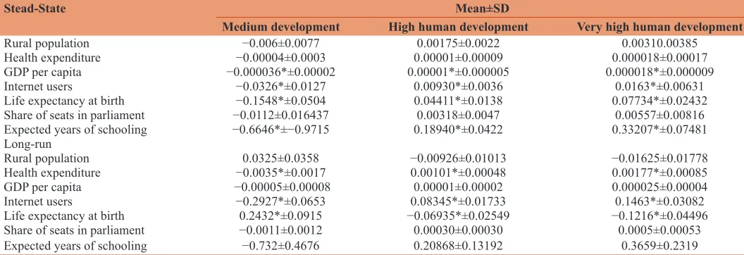
While other variables are fixed, the increase in expected years of schooling decreases the probability of having a medium development level by 66%. It increases the likelihood of having a high level of development by 19%. As life expectancy at birth

Table 2: Dependent and independent variables used in the study

Variables Description

HDI (dependent variable) HDI values of 130 countries between the years 2009-2014 (0.944-0.798=very high HDI, 0.798-0.721=high HDI and 0.721-0.575=medium HDI

Rural population, female (% of total) Female rural population is the percentage of females who live in rural areas to total population Health expenditure, private (% of GDP) Private health expenditure includes direct household (out-of-pocket) spending, private insurance,

charitable donations, and direct service payments by private corporations

GDP per capita (PPP$) Aggregate income of an economy generated by its production and its ownership of factors of

production, less the incomes paid for the use of factors of production owned by the rest of the world, converted to international dollars using PPP rates, divided by midyear population Internet users People with access to the worldwide network. (% of population)

Life expectancy at birth Life expectancy at birth indicates the number of years a newborn infant would live if prevailing patterns of mortality at the time of its birth were to stay the same throughout its life

Share of seats in parliament The proportion of seats held by women in national parliaments is the number of seats held by women members in single or lower chambers of national parliaments, expressed as a percentage of all occupied seats. (% held by women)

Expected years of schooling Number of years of schooling that a child of school entrance age can expect to receive if prevailing

patterns of age-specific enrolment rates persist throughout the child’s life

Source: Adapted from “UNDP human development report 2009-2014” and World Bank Wep page (http://hdr.undp.org/, http://databank.worldbank.org/data/home.aspx). HDI: Human development ındex, GDP: Gross domestic product

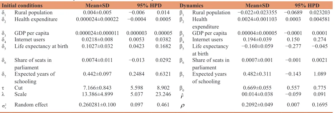
Table 3: Posterior summary for dynamic latent ordered probit model

Initial conditions Mean±SD 95% HPD Dynamics Mean±SD 95% HPD

δ₁ Rural population 0.004±0.005 −0.006 0.014 β₁ Rural population −0.022±0.023355 −0.0689 0.023203 δ₂ Health expenditure 0.000024±0.00022 −0.0004 0.0005 β₂ Health

expenditure 0.0024±0.001103 0.0003 0.004581

δ₃ GDP per capita 0.000024±0.000011 0.000003 0.00005 β₃ GDP per capita 0.00004±0.00005 −0.0001 0.0001 δ₄ Internet users 0.0218±0.008 0.0053 0.0382 β₄ Internet users 0.194±0.039 0.150 0.274 δ₅ Life expectancy at birth 0.1027±0.032 0.0423 0.1682 β₅ Life expectancy

at birth −0.160±0.059 −0.277 −0.045

δ₆ Share of seats in

parliament 0.0074±0.011 −0.013 0.0292 β6 Share of seats in parliament 0.0007±0.001 −0.001 0.0021

δ₇ Expected years of

schooling 0.442±0.097 0.2484 0.6321 β7 Expected years of schooling 0.482±0.311 −0.143 1.089

τ Cut 7.166±0.843 5.598 8.902 β₀ 0.669±0.055 0.557 0.775 λ Scale 13.386±4.899 5.037 23.246 _rˆ 00.014±0.038 −0.059 0.091

2

ε

σ Random effect 0.260281±0.100 0.097 0.461 ρ 0.2092±0.049 0.007 0.1695

Note: Based on 17600 MCMC draws. Threshold τ1 fixed at 0.σε2, indicates random effect. The accidental effect difference, estimated as 0.26, emphasizes the importance of controlling

increases, it increases the likelihood of having a very high level of development by 33%. The strong effect of expected years of schooling on human development continues in the long term.

While other variables are fixed; the increase in the life expectancy at birth decrease the likelihood of having medium level of development by 16%. It increases the probability of having a high level of development by 4%. As the increases, it increases the probability of having a very high level of development by 8%. The increase in life expectancy at birth affects the growth level of a country negatively in long term.

Women’s share of seats in parliament has a positive effect on the level of development in short and long terms. This effect in long term is less than that in short term.

5. CONCLUSION

In this study, Bayesian panel ordered probit model was estimated in order to determine the factors affecting the levels of development of 130 countries with moderate development, high development and very high development HDI values according to the human development reports.The main usage purpose of the Bayesian approach is to investigate the short- and long-term effects of human development level through many variables.

In the Bayesian ordered probit model, there is a positive correlation in short term between the variables of health expenditure, GDP, internet users, life expectancy at birth, share of expected years of schooling seats in parliament and HDI. In the long term, there is a negative correlation between the variables of rural population and life expectancy at birth and human development index, and positive correlation between other variables and HDI.

The results suggest that,internet use and GDP per capita are statistically significant at the level of development of the 130 analyzed countries. In the case of an increase in the expected

years of schooling, life expectancy at birth and internet use, the probability of increase in the level of development of countries also increases. The countries with moderate, high HDI values can concentrate on long and healthy life, access to information and especially education dimension in order to reach to the standards of the best countries, and accordingly design their policies.

REFERENCES

About Human Development. (2016), Available from: http://www.hdr. undp.org/en/humandev#humandev. [Last accessed on 2017 Jul 19]. Abayomi, K., Pizarro, G. (2013), Monitoring human development goals:

A straightforward (Bayesian) methodology for cross-national indi_ces.

Social Indicators Research, 110(2), 489-515.

Albert, J.H., Chib, S. (1993), Bayesian analysis of binary and polychotomous response data. Journal of the American Statistical Association, 88(422), 669-679.

Anand, S., Sen, A. (2000), The income component of the human development index. Journal of Human Development, 1(1), 83-106. Biagi, B., Ladu, M.G., Royuela, V. (2016), Human development and

tourism specialization. Evidence from a panel of developed and developing countries. International Journal of Tourism Research,

19, 160.

Blanchflower, D.G., Oswald, A.J. (2005), Happiness and the human development index: The paradox of Australia. Australian Economic Review, 38(3), 307-318.

Byun, H., Lee, C.Y. (2017), Analyzing Korean consumers’ latent

preferences for electricity generation sources with a hierarchical

Bayesian logit model in a discrete choice experiment. Energy Policy, 105, 294-302.

Davies, A. (2009), Human development and the optimal size of government. The Journal of Socio-Economics, 38(2), 326-330. Davies, A., Quinlivan, G. (2006), A panel data analysis of the impact

of trade on human development. The Journal of Socio-Economics,

35(5), 868-876.

Eren, M., Çelik, A.K., Kubat, A. (2014), Determinants of the levels of development based on the human development index: A comparison

of regression models for limited dependent variables. Review of

European Studies, 6(1), 10.

Franses, P.H., Cramer, J.S. (2010), On the number of categories in an

Table 4: Steady-state and long-run effects

Stead-State Mean±SD

Medium development High human development Very high human development

Rural population −0.006±0.0077 0.00175±0.0022 0.00310.00385

Health expenditure −0.00004±0.0003 0.00001±0.00009 0.000018±0.00017

GDP per capita −0.000036*±0.00002 0.00001*±0.000005 0.000018*±0.000009

Internet users −0.0326*±0.0127 0.00930*±0.0036 0.0163*±0.00631

Life expectancy at birth −0.1548*±0.0504 0.04411*±0.0138 0.07734*±0.02432

Share of seats in parliament −0.0112±0.016437 0.00318±0.0047 0.00557±0.00816

Expected years of schooling −0.6646*±−0.9715 0.18940*±0.0422 0.33207*±0.07481

Long-run

Rural population 0.0325±0.0358 −0.00926±0.01013 −0.01625±0.01778

Health expenditure −0.0035*±0.0017 0.00101*±0.00048 0.00177*±0.00085

GDP per capita −0.00005±0.00008 0.00001±0.00002 0.000025±0.00004

Internet users −0.2927*±0.0653 0.08345*±0.01733 0.1463*±0.03082

Life expectancy at birth 0.2432*±0.0915 −0.06935*±0.02549 −0.1216*±0.04496

Share of seats in parliament −0.0011±0.0012 0.00030±0.00030 0.0005±0.00053

Expected years of schooling −0.732±0.4676 0.20868±0.13192 0.3659±0.2319

ordered regression model. Statistica Neerlandica, 64(1), 125-128. Gelman, A., Carlin, J.B., Stern, H.S., Dunson, D.B., Vehtari, A., Rubin, D.B.

(2014), Bayesian Data Analysis. Vol. 2. Boca Raton, FL: CRC Press. Greene, W.H. (2003), Econometric Analysis. 5th ed. Upper Saddle River,

NJ: New York University.

Greene, W.H., Hensher, D.A. (2010), Modeling Ordered Choices: A Primer. New York: Cambridge University Press.

Grimm, M., Harttgen, K., Klasen, S., Misselhorn, M. (2008), A human

development index by income groups. World Development, 36(12),

2527-2546.

Hasegawa, H. (2009), Bayesian dynamic panel-ordered probit model and its application to subjective well-being. Communications in Statistics-Simulation and Computation, 38(6), 1321-1347. Heckman, J.J. (1978), Dummy endogeneous variables in a simultaneous

equation system. Econometrica, 46, 931-959.

Hou, J., Walsh, P.P., Zhang, J. (2015), The dynamics of human development index. The Social Science Journal, 52(3), 331-347. Johnson, E. (2008), Subjective Well-Being and Human Development.

New Brunswick: Mt. Allison University, Mimeo.

Johnson, V.E., Albert, J.H. (1999), Ordinal Data Modeling. New York:

Springer.

Lee, H.S., Lin, K., Fang, H.H. (2006), A fuzzy multiple objective DEA for the human development index. In: International Conference on Knowledge-Based and Intelligent Information and Engineering Systems. Berlin, Heidelberg: Springer. p922-928.

McCulloch, R., Rossi, P.E. (1994), An exact likelihood analysis of the multinomial probit model. Journal of Econometrics, 64(1), 207-240. Müller, G., Czado, C. (2005), An autoregressive ordered probit model

with application to high-frequency financial data. Journal of

Computational and Graphical Statistics, 14(2), 320-338.

Portnoi, L.M. (2016), Policy Borrowing and Reform in Education: Globalized Processes and Local Contexts. New York: Springer. Pudney, S. (2008), The dynamics of perception: Modelling subjective

wellbeing in a short panel. Journal of the Royal Statistical Society:

Series A (Statistics in Society), 171(1), 21-40.

Rabe-Hesketh, S., Skrondal, A. (2008), Generalized linear mixed-effects models. Longitudinal Data Analysis. Boca Raton, FL: Chapman and Hall/CRC. p79-106.

Sagar, A.D., Najam, A. (1998), The human development index: A critical review. Ecological Economics, 25(3), 249-264.

Sharma, H., Sharma, D. (2015), Human development index-revisited:

Integration of human values. Journal of Human Values, 21(1), 23-36.

Stegmueller, D. (2013), Modeling dynamic preferences: A Bayesian robust dynamic latent ordered probit model. Political Analysis,

21(3), 314-333.

UNDP. (2016a), Human Development İndex. Available from: http://www. hdr.undp.org/en/reports/about. [Last retrieved on 2015 Sep 25]. UNDP. (2016b), Human Development İndex. Available from: http://

www.hdr.undp.org/en/humandev#humandev. [Last retrieved on