5REXVWVSDUVHSULQFLSDOFRPSRQHQWDQDO\VLV
&KULVWRSKH&URX[3HWHU)LO]PRVHUDQG+HLQULFK)ULW]
DEPARTMENT OF DECISION SCIENCES AND INFORMATION MANAGEMENT (KBI)
Robust Sparse Principal Component Analysis
Christophe Croux
K.U. Leuven
Peter Filzmoser
Vienna University of Technology
Heinrich Fritz
Vienna University of Technology
Abstract
A method for principal component analysis is proposed that is sparse and robust at the same time. The sparsity delivers principal components that have loadings on a small number of variables, making them easier to interpret. The robustness makes the analysis resistant to outlying observations. The principal components correspond to directions that maximize a robust measure of the variance, with an additional penalty term to take sparseness into account. We propose an algorithm to compute the sparse and robust principal components. The method is applied on several real data examples, and diagnostic plots for detecting outliers and for selecting the degree of sparsity are provided. A simulation experiment studies the loss in statistical efficiency by requiring both robustness and sparsity.
Keywords: dispersion measure, projection-pursuit, outliers, variable selection
1
Introduction
Principal component analysis (PCA) is a standard tool for dimension reduction of multivariate data. PCA searches for linear combinations of the variables, called principal components (PC), that summarize well the data. The PCs correspond to directions maximizing the variance of the data projected on them (see, e.g. Jollife, 2002). The transformation matrix defining the principal components is called the loadings matrix, and it may be used to interpret the PCs. In general, PCA does not deliver well interpretable components. Good interpretability of PCs is related to rather large or small (absolute) values in the loadings matrix yielding either quite strong or quite weak contributions of the variables to the PC. Loadings matrices with many values exactly equal to zero, which we call sparse loadings matrices, are preferred, since the interpretation of a particular
principal component does not require to consider all variables, but only a small subset. This yields a sparse PCA, which is especially helpful for analyzing high dimensional data sets. In this paper we introduce a method for PCA that yields both sparse and robust results. Outliers frequently occur in multivariate data sets, and any multivariate procedure should take the possible presence of outliers into account.
Different approaches for computing sparse loadings matrices have been proposed in the litera-ture. Vines (2000) and Anaya-Izquierdo et al.(2011) use a restriction on the loadings to integers. Jolliffe et al. (2003) introduced the SCoTLASS, related to the Lasso estimator (Tibshirani, 1996). Here the principal components maximize the variance but under an upper bound on the sum of the absolute values of the loadings. It is shown that such an approach yields better results than a two-step procedure, where after a standard PCA rotation techniques are performed (Jollife, 1995). Zouet al.(2006) use the elastic net to obtain a version of sparse PCA. Modifications and improve-ments of this method are made in Leng and Wang (2009). Finally, Guo et al. (2011) introduce a fusion penalty to capture block structures within the variables. All these methods, however, are not robust to outliers.
This paper proposes a PCA method that is robust and sparse at the same time. Several robust, but non sparse, PCA methods have been introduced in the literature (see, e.g., Filzmoser, 1999; Hubert et al., 2005; Maronna, 2005), and robustness properties were investigated (Croux and Haesbroeck, 2000). Here we focus on the projection-pursuit approach to PCA, where the PCs are extracted from the data by searching for directions that maximize a robust measure of variance of the data projected on it (Li and Chen, 1985; Croux and Ruiz-Gazen, 2005). Using a robust measure of variance avoids that the PCs are attracted by the outliers, since outliers inflate the standard non-robust variance. An efficient algorithm for computing the projection-pursuit based PCs is the Grid algorithm, introduced in Crouxet al. (2007). The Grid algorithm is very precise, and an implementation is available in the R package pcaPP (Filzmoser et al., 2010). Up to the best of our knowledge, the PCA method we propose is the first one combining the properties of robustness and sparsity.
The paper is organized as follows: Section 2 defines the robust sparse principal components as the solution of a non convex optimization problem. Section 3 shows how the Grid algorithm can be extended to find an approximate solution of this problem. The selection of tuning parameters
is discussed in Section 4. Simulation results are presented in Section 5, and real data examples are shown in Section 6. The final Section 7 concludes.
2
Method
Given n multivariate observations x1, . . . ,xn ∈ Rp, collected in the rows of the data matrix X.
The first PCA direction is given by
a1 = argmax kak=1
V(atx1, . . . ,atxn), (1)
where V is a variance measure. In the standard non-robust case, V is the empirical variance (Var), and the resulting optimal direction a1 corresponds to the first eigenvector of the sample
covariance matrix. Equation (1) is the projection-pursuit formulation for finding the first PC, with V being the projection-pursuit index. Robust PCA directions can easily be obtained by taking a robust variance measure for V, like the squared Median Absolute Deviation (MAD) or the squaredQnestimator. TheQnestimator was proposed in Rousseeuw and Croux (1993) and is,
for a univariate data sety1, . . . , yn, defined as the first quartile of all pairwise distances|yi−yj|, for
1 ≤i < j ≤ n. Croux and Ruiz-Gazen (2005) showed that using the Q2
n estimator as projection
index yields robust and efficient estimates for the principal components. In the remainder of this paper, we use the Q2
n as robust variance estimator.
Suppose the firstj−1 PCA directions have already been found (j >1), then thejth direction (j ≤p) is defined as
aj = argmax
kak=1,a⊥a1,...,a⊥aj−1
V(atx1, . . . ,atxn), (2)
imposing an orthogonality constraint to all previously found directions. The jth principal com-ponent is then the vector containing the PCA scores
zij =atjxi for i= 1, . . . , n. (3)
The loadings matrix for the first k PCs is denoted byAk, and contains in its columns the optimal directions or loadings vectors aj, for 1≤j ≤k. The loadings determine the contribution of each variable to the principal components. The matrix containing the principal component scores is then
Sparsity can be imposed on the PCA directions by adding an L1 penalty in the objective
function. As such, Jolliffe et al.(2003) introduced the SCoTLASS criterion, max
kak=1,a⊥a1,...,a⊥aj−1
atΣˆa, subject tokak1 ≤t, (5)
for obtaining the jth PCA direction, with 1≤j ≤p. Here, Σˆ is the empirical covariance matrix, and the L1 normkak1 =Ppj=1|aj| takes the sum of the absolute values of the components of the
vector a. It is more convenient to work with the dual formulation of the above problem, given by max
kak=1,a⊥a1,...,a⊥aj−1
atΣˆa−λ1kak1, (6)
where λ1 is a tuning parameter. The larger λ1, the more the components of a are shrunken
towards zero. Due to the use of the L1 penalty, some of the loadings will even become exactly
zero, similar as for the Lasso estimator in regression. The approach of Jolliffeet al.(2003) requires an estimated covariance matrixΣˆ as input of the maximization problem (5), which can be solved using the algorithm detailed in Trendafilov and Jolliffe (2006) or in Journ´ee et al. (2010).
An obvious way to sparse robust PCA would be to replace the empirical covariance matrix by a robust covariance estimator, as is often done in robust multivariate data analysis (Hubert
et al., 2008). However, computing robust covariance matrices in high dimensions, and particularly if p > n, is cumbersome –the estimator may even not exist– and time consuming. We therefore propose to stick to the projection-pursuit approach, where the PCs are directly obtained without using a prior covariance estimation. Adding the L1 constraint in definition (1) for finding the first
PCA direction yields
˜
a1 = argmax kak=1
V(atx1, . . . ,atxn)−λ1kak1. (7)
The vector ˜a1 is the first sparse PCA direction, and its sparsity is controlled by the tuning
parameterλ1. Settingλ1 = 0 results in the unconstrained first PCA directiona1, but for increasing
values of λ1, sparsity gains importance compared to robust variance maximization. Similarly, the
jth sparse PCA direction (1< j ≤p) is defined by
˜
aj = argmax
kak=1,a⊥˜a1,...,a⊥a˜j−1
V(atx1, . . . ,atxn)−λjkak1, (8)
withλj a tuning parameter, possibly different fromλ1. Definition (7) and (8) are very elegant and
maximizing a robust variance, under the constraint the loadings should not become too large. If
V = Var, then definitions (6) and (7) are the same. Note that most often one does not need all possible PCs, but only the first few. An advantage of the projection-pursuit approach is that the estimators are computed sequentially, reducing the computation time for small values of k.
3
Algorithm
Computing the projection-pursuit based PCs requires to find the optimal directions in (1) and (2) over a p-dimensional space. For general projection indices V it is not possible to find analytical solutions for the optimal directions. Moreover, sinceV may be not differentiable in its arguments, using gradient based methods is not always possible. Several proposals to find good approximations of the projection-pursuit based PCs, applicable for any choice of the projection indexV, have been made (Hubert et al., 2002; Croux and Ruiz-Gazen, 2005; Croux et al., 2007). In this paper we extend the Grid algorithm of Croux et al. (2007) for obtaining sparse solutions, i.e. to solve (7) and (8). The algorithm is fast to compute and accurate even for larger dimension. It is available in the R package pcaPP (Filzmoser et al., 2010). Below we give an outline of the algorithm.
Let k be the number of sparse PCs that need to be computed. Assume that the first j −1 sparse PCA directions ˜aj−1 are already obtained and are collected in the first j −1 columns of
the loadings matrix Aj˜ −1, with 1 ≤ j ≤ k −1. Now we want to compute ˜aj. For notational
consistency, set A˜⊥0 equal to the identity matrix. For j > 1, let A˜⊥j−1 be a matrix containing in
its columns an orthonormal basis for the subspace orthogonal to the space spanned by the first
j −1 sparse PCA directions. Denote x(ij−1) = (A˜⊥j−1)tx
i, for i= 1, . . . , n, belonging to the
lower-dimensional spaceRp−j+1. Solving the maximization problem (8) is then equivalent to maximizing
the objective function
f(a) = V(atx(1j−1), . . . ,atx(nj−1))−λjkA˜
⊥
j−1ak1, (9)
under the restriction that kak= 1. As sparseness relates to the components of a direction in the space of the original variables, and not to the lower dimensional space a belongs to, we need to back-transform the vector a to the original space before taking the L1 norm.
For optimizing (9) the Grid algorithm is used. The basic idea of this algorithm is to reduce the problem to a sequence of optimizations in a two-dimensional plane under a unit norm constraint.
This boils down to a sequence of maximizations of a function over the unit circle, which is simply a univariate maximization problem that can be solved by means of a grid search over [−π, π]. Consider the optimization of (9) for a given value of 1≤j ≤k. We take the following steps:
1. Sort the columns of X(j), where the rows of X(j) contain the vectors x(ij−1), in descending order of their projection index V. Then the first variable has the largest value for V and its corresponding loadings vector a = (1,0, . . . ,0) serves as a first approximation of the solution. The vector a has p−j + 1 components.
2. For l = 1, . . . , maxiter, perform an iteration step in which all components of the vector a
are updated
• For 1≤i≤p−j+ 1, update theith component,ai, of the current best approximation a by finding the angle γ∗ maximizing
f¡a1b(γ), . . . , ai−1b(γ),cosγ, ai+1b(γ), . . . , ap−j+1b(γ)¢,
where γ ranges in the interval [arccos(ai)−π/(2l−1),arccos(ai) +π/(2l−1)], and where
b(γ) = sin(γ)/p1−(ai)2 is such that the unit norm condition holds. This function is
maximized by a grid search using N gridevaluation points. The updated value of ai is
then simply cosγ∗.
Note that if the iteration stepl increases, we perform a more restricted search in the plane, since we assume that we are already close enough to the solution. Since N grid remains constant, we are increasing the precision in every iteration step.
The procedure is said to converge when the absolute change of the optimal directionabetween two iterations drops below a prespecified tolerance level. The procedure always stops if the maximum number of iterations (maxiter) is reached. In our implementation, we take N grid = 25 and
maxiter = 10 by default. Finally, the optimal sparse directiona found for thejth PC by the grid algorithm has to be back-transformed into the original space, yielding aj˜ =A˜⊥j−1a.
4
Selection of
λ
The tuning parameterλj regulates the degree of sparseness. The largerλj, the less weight is given
relative importance of the penalty term in (8) comparable across the different PCs, i.e. to have a similar degree of sparsity over the different principal components, we take
λj :=λV(X(j)), (10)
where the matrixX(j)is defined in the previous section, and contains the data vectors projected on the orthogonal complement of the space spanned by the firstj−1 optimal directions. Furthermore, V denotes the total robust variance of a data matrix, and is for anyn by p matrix Y defined as
V(Y) =
p
X
i=1
V(yi), (11)
where yi stands for the ith column of Y and V is the robust variance measure used as projection
index. Using (10), there is only one tuning parameter λ to be selected. The penalty term λj
decreases with increasing j, along with the value of the projection index V for the jth principal component.
We propose to select the λ to minimize a BIC type criterion (see also Guo et al., 2011; Leng and Wang, 2009)
BIC(λ) = RVf
RV + df(λ) log(n)
n , (12)
whereRV and RV refer to the total robust variance of the residuals matrix obtained from a sparsef PCA and an unconstrained PCA. The first term in the BIC is a measure for the quality of the fit, while the second term penalizes for model complexity. Here, df(λ) is the number of non-zero loadings when using λ as the penalty parameter, as in Guo et al. (2011). The calculation of RVf and RV is immediate, since they are given by
f
RV =V(X −XAk˜ A˜kt) and RV =V(X −XAkAtk),
where X stands for the data matrix, andAk and Ak˜ denote the loadings matrices containing the first k PC directions (in the columns) for unconstrained and constrained PCA, respectively. Note that, for V = Var, the BIC criterion in (12) equals the one in Guo et al. (2011). In practice, the selection of λ is carried out by minimizing the BIC(λ) over a grid [0, λmax], where λmax results in
full sparseness of the sparse PCA solution with k components (i.e. every loadings vector contains only one non-zero element).
Besides λ, one also needs to choose the number of components k. Appropriate selection of k
made for it. In this paper we select the numberkfrom the scree-plot of an unconstrained PCA (see Cattell, 1966). Such a scree-plot represents the percentage of explained (robust) variance (EV) by the PCs versus the number of principal components. Mathematically, the explained (robust) variance is given by
EVk = V
(Zk)
V(X), (13)
with Zk the matrix containing the principal component scores, see (4). ForV = Var, EVk equals
the ratio of the sum of the k largest eigenvalues to the sum of all eigenvalues of the sample covariance matrix. Since we are concerned about ease of interpretation and sparsity we do not want to select a higher number of components when running the Sparse PCA, and maintain the same number of PCs. For this value ofk, a selectedλshould result in a sparser loadings matrix, at the price of limited reduction in explained (robust) variance. In Section 6 we present the so-called
tradeoff curve, where the percentage of explained variance of the k sparse PCs is plotted as a function of λ. This tradeoff curve is a graphical tool, in addition to the BIC, for selecting an appropriate value of λ.
5
Simulation experiments
In this section we present two simulation experiments. The sparse method should (i) result in increased estimation precision when the true loadings matrix is sparse, and (ii) succeed in detecting those variables that do not contribute to the principal components, i.e. true zero loadings are exactly estimated as zero. We contrast the standard approach, with V = Var, with the robust approach, with V =Q2
n. If no outliers are present, then the two properties above hold for both
approaches. But it will be shown that, in presence of outliers, the standard sparse method does not meet its objectives anymore.
Experiment 1
We generate data sets of n = 50 observations inp= 10 dimensions. The true loadings matrix is
A= √ 0.5 0 √ 0.5 0 0 · · · 0 √ 0.5 0 − √ 0.5 0 0 · · · 0 0 √0.5 0 √ 0.5 0 · · · 0 0 √0.5 0 − √ 0.5 0 · · · 0 0 0 0 0 1 0 .. . ... ... ... . .. 0 0 0 0 0 1
and the eigenvalues are l= (1,0.5,0.1, . . . ,0.1).The observations are generated from a multivari-ate normal distribution N10
¡
0,ALAt¢, with a diagonal matrix L holding the values of l in its diagonal. Contamination is added by replacing a portion of pout observations by outliers,
gener-ated from the distribution N10(µout,I10) with µout = (2,4,2,4,0,−1,1,0,1,−1) t
. Note that the outliers are not very far from the center of the model distribution. From the generated data set the loadings matrix is estimated, with k = 2. The resulting Aˆ2 is compared to the true A2,
containing the first two columns of A, by computing the angle ϕ between the subspaces spanned by columns of the matrices.
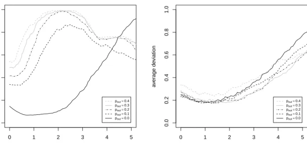
Both the standard and the robust sparse PCA procedure are applied to m = 100 simulated data sets. Figure 1 pictures the average value of ϕ over the m simulations, as a function of the tuning parameter λ. Different outlier proportions, ranging from no contamination to 40% of outliers are considered.
If no outliers are present (pout = 0, solid line), we get the expected pattern. Starting with
λ = 0 (i.e. non sparse PCA) the estimation error decreases until a minimum is reached at about
λ = 1.2. Penalizing the loadings further yields again an increasing estimation error. If the true model is sparse (here about 80% of the true loadings are zero) sparse estimation methods indeed may improve the precision of the maximum likelihood method. For the robust sparse method a similar pattern is observed. Note that there is a slight loss in precision using the robust instead of the standard method. However, the robust method remains fairly accurate under contamination, as can be seen from the other curves in Figure 1 (b). This is in contrast with the standard method, where the estimation error increases substantially and supersedes those of the robust counterpart
0 1 2 3 4 5 0.0 0.2 0.4 0.6 0.8 1.0
(a) Standard sparse PCA
λ a v er age de viation pout=0.4 pout=0.3 pout=0.2 pout=0.1 pout=0.0 0 1 2 3 4 5 0.0 0.2 0.4 0.6 0.8 1.0
(b) Robust sparse PCA
λ a v er age de viation pout=0.4 pout=0.3 pout=0.2 pout=0.1 pout=0.0
Figure 1: Average deviation between estimated and true loadings for (a) the standard and (b) robust sparse PCA methods for different levels of contamination pout and different values of λ.
by a large amount. Finally, note that in presence of outliers the advantage of penalizing disappears for the standard method, sinceλ = 0 yields the smallest average deviationϕ. This does not happen for robust sparse PCA.
Experiment 2
We consider the same design as introduced by Zou et al. (2006), and subsequently used by Far-comeni (2009) and Guo et al. (2011) in the same context of sparse PCA. We have n = 20 obser-vations and p= 10 variables driven by two latent variables
U1 ∼N(0,290), U2 ∼N(0,300),
where ε∼N(0,1), andU1, U2 and ε are independent. The observed variables are constructed as
Xj = U1 +εj, if 1≤j ≤4 U2 +εj, if 5≤j ≤8 −0.3U1+ 0.925U2 +ε+εj, if j = 9,10.
The error terms ε and εj, for 1 ≤ j ≤ 10, are i.i.d. N(0,1). The first two principal
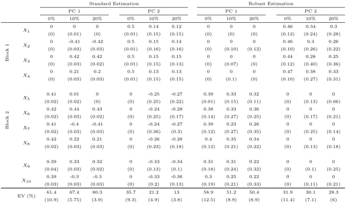
Table 1: Second simulation experiment: simulated loadings of the 10 variables on the first two PCs using standard and robust sparse PCA. The last line presents the percentage of explained variance EV. The reported values are the median and MAD (in parenthesis) over 100 simulation runs. The different columns correspond to no outliers (“0%”), and 10% and 20% of outliers in the data.
Standard Estimation Robust Estimation
PC 1 PC 2 PC 1 PC 2 0% 10% 20% 0% 10% 20% 0% 10% 20% 0% 10% 20% B lo c k 1 X1 0 0 0 0.5 0.14 0.12 0 0 0 0.46 0.34 0.3 (0) (0.01) (0) (0.01) (0.15) (0.15) (0) (0) (0) (0.12) (0.24) (0.28) X2 0 -0.41 -0.42 0.5 0.15 0.14 0 0 0 0.46 0.3 0.26 (0) (0.03) (0.03) (0.01) (0.16) (0.16) (0) (0.10) (0.12) (0.10) (0.26) (0.22) X3 0 0.42 0.42 0.5 0.15 0.15 0 0 0 0.44 0.28 0.25 (0) (0.03) (0.02) (0.01) (0.15) (0.13) (0) (0.07) (0) (0.12) (0.40) (0.36) X4 0 0.21 0.2 0.5 0.13 0.13 0 0 0 0.47 0.38 0.33 (0) (0.03) (0.03) (0.01) (0.15) (0.15) (0) (0.1) (0) (0.10) (0.27) (0.31) B lo c k 2 X5 0.41 0.01 0 0 -0.25 -0.27 0.39 0.33 0.32 0 0 0 (0.02) (0.02) (0) (0) (0.25) (0.22) (0.01) (0.15) (0.11) (0) (0.13) (0.06) X6 0.42 0.44 0.43 0 -0.24 -0.28 0.38 0.33 0.36 0 0 0 (0.02) (0.03) (0.02) (0) (0.25) (0.17) (0.14) (0.27) (0.25) (0) (0.17) (0.21) X7 0.41 -0.4 -0.41 0 -0.24 -0.27 0.39 0.23 0.26 0 0 0 (0.02) (0.03) (0.03) (0) (0.36) (0.3) (0.12) (0.27) (0.35) (0) (0.25) (0.14) X8 0.42 0.22 0.21 0 -0.26 -0.28 0.4 0.35 0.34 0 0 0 (0.02) (0.03) (0.03) (0) (0.23) (0.18) (0.12) (0.21) (0.22) (0) (0.13) (0.18) X9 0.39 0.33 0.32 0 -0.33 -0.34 0.31 0.31 0.22 0 0 0 (0.04) (0.03) (0.02) (0) (0.13) (0.1) (0.18) (0.24) (0.32) (0) (0.1) (0.25) X10 0.39 -0.3 -0.3 0 -0.33 -0.36 0.3 0.25 0.22 0 0 0 (0.03) (0.03) (0.03) (0) (0.2) (0.13) (0.19) (0.21) (0.33) (0) (0.11) (0.21) EV (%) 61.4 67.4 80.3 35.7 21.2 13 58.9 51.2 50.4 31.9 30.1 28.3 (10.9) (5.75) (3.9) (9.3) (4.9) (3.8) (12.5) (8.9) (8.9) (11.4) (7.1) (6)
X1 to X4 is expected to have a high loading on the second PC, but zero loadings on the first
one. The second block, X5 to X8, should have important loadings on the first PC, but a
zero loading on the second one. The remaining variables X9 and X10 have a more important
loading on the first PC than on the second one, and a sparse PCA could shrink this second loading to zero. We will add outliers generated from the distribution N(µout, σ2
outI10), with
µout = (0,−100,100,50,0,100,−100,50,75,−75)t, and σout2 = 20. These added data are not
univariate outliers, and hence are not detectable by making boxplots of the individual variables, but they do not follow the factor structure described above.
We generate m = 100 samples according to the simulation design, using outlier portions 0%, 10%, and 20%, and apply the standard and the robust version of the sparse PCA algorithm. For every sample, an optimal value of the tuning parameter was selected according to the BIC
criterion. Then loadings of each of the 10 variables on the first two PCs are computed, as well as the percentage of explained (robust) variance EV. The reported values correspond to the median and median absolute deviation (MAD, between parenthesis) over the 100 replications, and are presented in Table 1, in a similar way as in (Guo et al., 2011, Table 1).
Without contamination (0 %), the results are according to the expectations, and very much comparable to those of Guo et al. (2011). For both the standard and the robust sparse method, we get that variables X5 throughX10 are solely represented in the first PC, variablesX1 toX4 in
the second PC , and the loadings of the last two variables for the second PC are also shrunken to zero. When adding contamination it is seen from Table 1 that the standard PCA gets distorted, and does not succeed in retrieving the sparsity in the data generating process. The robust method, however, still delivers sparse solutions. The price the robust method pays for the resistance with respect to outliers is an increased variability, as measured by the MAD values.
The standard sparse PC directions are attracted by the outliers and do no longer explain the actual structure of the majority of observations. As we can see from the last row of Table 1, the explained variance by the first principal component increases substantially with an increasing level of contamination. This is a misleading outcome, since it is only caused by the use of the sample variance estimator, which gets inflated due to the outliers. It is not meaning that the PCs are more representative for the bulk of the data. When using robust sparse PCA, we see that the percentage of explained variance remains about the same when the outliers are added.
6
Real data examples
The method is used for two differently structured data sets. The first example has n > p and shows how the robust method is capable of spotting groups of outliers. The second example points out the method’s applicability on high-dimensional data sets, where p > n.
Example 1
The car data set (Kibler et al., 1989) consists of 26 variables containing technical and insurance-related data for 205 different car models. Only continuous variables, and observations without missing values are considered here, resulting in a data set of size 195×14. To make the scale of
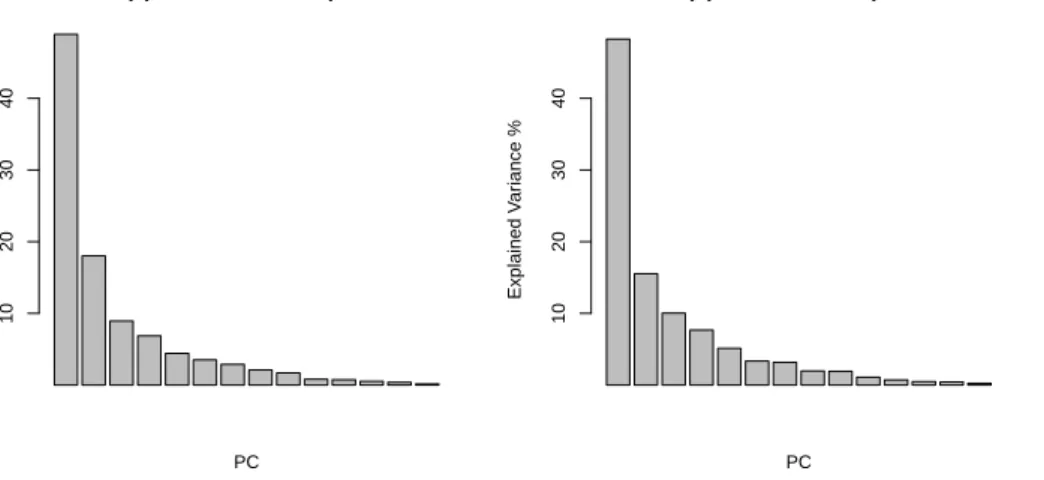
(a) Standard Scree−plot PC Explained V ar iance % 10 20 30 40 (b) Robust Scree−plot PC Explained V ar iance % 10 20 30 40
Figure 2: Scree-plots for a (a) standard and (b) robust PCA (λ = 0) for the car data set.
the variables comparable, we divide each column of the data matrix by its standard deviation (if
V = Var) or by a robust scale measure (if V = Qn). Figure 2 gives a scree-plot for non-sparse
standard and robust PCA, which plots the explained variance, as defined in (13), versus the number of components. Based on this scree-plot we decide to retain the first four PCs, explaining about 80% of the total (robust) variance, for both approaches.
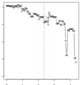
Figure 3 shows the tradeoff curve, discussed in Section 4, plotting the percentage of explained variance as a function of λ. The explained variances are computed over a grid of 100 different values of the tuning parameterλ, ranging fromλ= 0 (no sparseness) up to full sparseness (exactly one non-zero loading per PC). This plot illustrates how an increase in sparseness affects, and in general will lower, the explained variance. The idea is that the selectedλ should be such that the sharpest decline of tradeoff curve occurs afterwards. The selected λ should be close to the end of the first, relatively flat, part of the tradeoff curve. Using the BIC criterion from equation (12), minimized over the same grid of 100 values, we getλ= 2.36, corresponding to the vertical dashed line in the plot. From the tradeoff curve we conclude that this is an acceptable value. The sharper decline of the tradeoff curve occurs for a tuning parameter larger than 3.
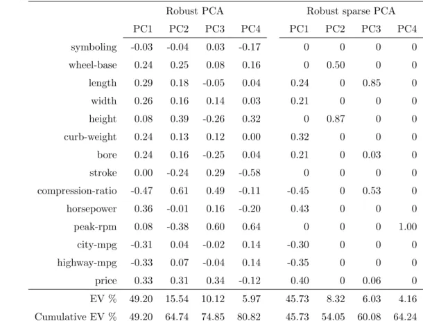
Table 2 shows the resulting loadings for robust non-sparse PCA and robust sparse PCA, derived with λ = 2.36. By adding the penalty term in the objective function, the number of non-zero loadings is reduced from 56 to 16, whereas the total amount of explained variance in the first four PCs drops from 81% to 64%. We do find this decrease in explained variance acceptable, given
0 1 2 3 4 0 20 40 60 80
Tradeoff curve (robust)
λ
Explained V
ar
iance %
Figure 3: Tradeoff curve for robust sparse PCA computed on the car data set. The dashed line represents the λ selected by the BIC criterion.
the gained sparsity in the loadings matrix. This could facilitate interpretation, in particular for the higher order principal components. For instance, the fourth principal component is uniquely determined by peak-rpm.
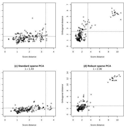
Further exploratory data analysis can be done by making distance-distance plots (see Hubert
et al., 2002). Such a plot presents two different distance measures: the score distance of each observation in the space of the firstk PCs, and the orthogonal distance of each observation to this space. Using cut-off values for both types of distances, outliers can be identified that do not follow the pattern the majority of the data follows. For details on the construction of these plots, we refer to Hubertet al.(2002). Figure 4 shows distance-distance plots for the car data, using standard and robust PCA, and their sparse versions, resulting in four different plots. As before, the first k = 4 PCs are retained, andλis selected according to the BIC. The robust distance-distance plot (Figure 4b) points out a very distinct outlier group (denoted by symbols ×) which in fact represents all car-models running on diesel. The robust sparse model (Figure 4d) is also able to clearly identify this particular group of outliers. In contrast, when considering the standard non-sparse (Figure 4a) and sparse (Figure 4c) distance-distance plots, these outliers cannot be identified, since their
Table 2: Loadings of the variables on the first four robust non-sparse (λ = 0) and robust sparse (λ= 2.36) PCs of the car data set.
Robust PCA Robust sparse PCA
PC1 PC2 PC3 PC4 PC1 PC2 PC3 PC4 symboling -0.03 -0.04 0.03 -0.17 0 0 0 0 wheel-base 0.24 0.25 0.08 0.16 0 0.50 0 0 length 0.29 0.18 -0.05 0.04 0.24 0 0.85 0 width 0.26 0.16 0.14 0.03 0.21 0 0 0 height 0.08 0.39 -0.26 0.32 0 0.87 0 0 curb-weight 0.24 0.13 0.12 0.00 0.32 0 0 0 bore 0.24 0.16 -0.25 0.04 0.21 0 0.03 0 stroke 0.00 -0.24 0.29 -0.58 0 0 0 0 compression-ratio -0.47 0.61 0.49 -0.11 -0.45 0 0.53 0 horsepower 0.36 -0.01 0.16 -0.20 0.43 0 0 0 peak-rpm 0.08 -0.38 0.60 0.64 0 0 0 1.00 city-mpg -0.31 0.04 -0.02 0.14 -0.30 0 0 0 highway-mpg -0.33 0.07 -0.04 0.14 -0.35 0 0 0 price 0.33 0.31 0.34 -0.12 0.40 0 0.06 0 EV % 49.20 15.54 10.12 5.97 45.73 8.32 6.03 4.16 Cumulative EV % 49.20 64.74 74.85 80.82 45.73 54.05 60.08 64.24
presence is masked by the use of a non-robust diagnostic measure. We conclude that in this example only the robust procedure allows to detect the group of outliers, and that adding the sparsity condition did not affected the diagnostic power of the robust distance-distance plot.
Example 2
The yarn data set (see Swierenga et al., 1999) contains near-infrared (NIR) spectra of 21 PET yarns of different density. 268 different wavelengths were measured, yielding a data set of size 21×268. As the algorithm discussed in Section 3 computes one (sparse) PC at a time and may stop after computing the kth component, it is especially useful in high-dimensional applications, where the actual information is restricted to a comparatively low-dimensional subspace. Due to this characteristic, computation time can be reduced tremendously, as in such settings usually only a few PCs are important. In the data set k = 2 PCs already explain more than 85% of the
0 1 2 3 4 0 1 2 3 4 5 6 7
(a) Standard PCA
Score distance Or thogonal distance 0 2 4 6 8 10 0 1 2 3 4 5 6 7 (b) Robust PCA Score distance Or thogonal distance 0 1 2 3 4 0 2 4 6 8 10 12 14
(c) Standard sparse PCA
Score distance Or thogonal distance λ =1.43 0 2 4 6 8 10 0 2 4 6 8 10 12 14
(d) Robust sparse PCA
Score distance
Or
thogonal distance
λ =2.36
Figure 4: Distance-distance plots for standard and robust PCA and their sparse versions. In the robust plots vehicles running on diesel (×) are clearly distinguishable from vehicles using gasoline (°).
total (robust) variance, thus the iteration can be stopped after obtaining the first two principal components, rather than computing all min(n, p) loadings vectors. In this particular example this reduces computation time by 90% (from 41 to 4 seconds for standard and from 135 to 13 seconds for robust PCA on an AMD Athlon x64 X2 4200+ running at 2.2GHz).
Figure 5 shows the spectral lines of the 21 observations (black). Three spectral intervals A, B and C are pointed out, as the variables in these areas show a higher variance than in other regions. In interval B the single yarns are grouped together to 5 “clusters”, whereas in region A and C this pattern cannot be observed and the yarns are more homogeneously structured. We add three
0 50 100 150 200 250 0 2 4 6 8 Wavenumber Intensity A B C
Figure 5: The yarn data set. The NIR spectrum of 21 different PET yarns (black), with intensity measured at 268 wavelengths. Outliers (in grey) were added for challenging the robust sparse PCA estimator.
outlying spectra (see Figure 5, in grey) in order to test the algorithm’s robustness properties in high-dimensional scenarios.
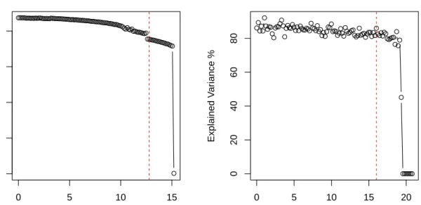
We start by selecting an appropriate value for the numberk of PCs to retain. The screeplot in Figure 6 conforms thatk = 2 is a good choice, explaining most of the (robust) variance. Note that the large value forEV1 for the standard method is mainly due to the fact that the sample variance
is inflated by the outliers. The screeplot for standard PCA on the data set without the outlying spectra does resemble Figure 6 (b). Then, we use the tradeoff curve in Figure 7 for selecting a value of λ keeping a sufficiently large percentage of explained variance. For robust PCA we take
λ = 16.02, a value at the end of the flat part of the curve and well before the sharp decrease in the tradeoff curve. For that value of λ we explain still 85% of the robust variance. The BIC criterion gives us a value of 19.55, which is not that different, but leads to a too large loss of explained robust variance. For standard PCA we take λ= 12.77 explaining 75% the total variance.
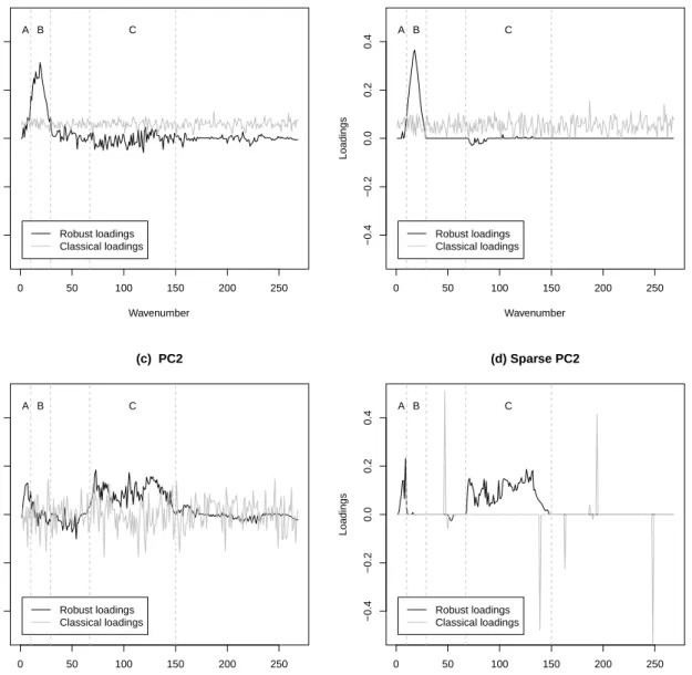
Figure 8 shows the loadings of the 268 variables, labeled with wavenumbers one to 268 for standard and robust PCA, and their sparse version. For standard PCA, the loadings in general
(a) Standard Scree−plot PC Explained V ar iance % 0.2 0.4 0.6 (b) Robust Scree−plot PC Explained V ar iance % 0.2 0.4 0.6
Figure 6: Scree-plots for a (a) standard and (b) robust PCA (λ= 0) for the yarn data set.
0 5 10 15 0 20 40 60 80
(a) Tradeoff curve (standard)
λ Explained V ar iance % 0 5 10 15 20 0 20 40 60 80
(b) Tradeoff curve (robust)
λ
Explained V
ar
iance %
Figure 7: Tradeoff curves for standard and robust sparse PCA computed on the yarn data set. The dashed lines represent the selected value of the tuning parameter λ.
do not seem to contain any interpretable structure and are heavily influenced by the outliers. The first standard sparse PC (panel b, dashed line), does hardly contain any zeros, whereas the second (panel d, dashed line) does only contain 11 non-zero loadings. However, this second sparse standard PC does not point out specific spectral ranges, but is mainly made up of single
0 50 100 150 200 250 −0.4 −0.2 0.0 0.2 0.4 (a) PC1 Wavenumber Loadings A B C Robust loadings Classical loadings 0 50 100 150 200 250 −0.4 −0.2 0.0 0.2 0.4 (b) Sparse PC1 Wavenumber Loadings A B C Robust loadings Classical loadings 0 50 100 150 200 250 −0.4 −0.2 0.0 0.2 0.4 (c) PC2 Wavenumber Loadings A B C Robust loadings Classical loadings 0 50 100 150 200 250 −0.4 −0.2 0.0 0.2 0.4 (d) Sparse PC2 Wavenumber Loadings A B C Robust loadings Classical loadings
Figure 8: Loadings of the 268 variables on the first two principal components using standard (grey) and robust (black) PCA. Results are given for both sparse (right) and non-sparse (left) PCA for the yarn data set.
spikes, describing the outlier’s random pattern. In contrast to this, robust PCA shows distinct features in all four plots. The first non-sparse robust PC (panel a, solid line) points out a peak at the spectrum’s lower end. This peak is even much more clearly detected by the robust sparse model (panel b, solid line) and corresponds to the spectral range B in which the yarns reveal a
rather “clustered” structure. Most of the loadings outside of the interval B are reduced to zero, illustrating that a sparse approach make interpretation easier. The second robust PC (panel c, solid line) is mainly made up of the wavelengths in spectral ranges A and C, corresponding to the wavelengths with high variability but without “cluster structure” among the yarns. Wavelengths outside of these intervals A and C contribute less to the second PC, as their (absolute) loadings are quite low. The loadings of the second sparse robust PC (panel d, solid line) do even much better in separating the wavelengths in intervals A or C from the others; almost all loadings outside of these ranges are exactly equal to zero. As we can see from the tradeoff curve in Figure 7 (b), the sparse robust solution only explains 1% less variance than the non-sparse (λ = 0), whereas the number of non-zero loadings decreases from 2×268 = 536 to 159. Despite the noise added by the three outlying spectra, the robust sparse method is capable of finding distinct structures in the data.
7
Concluding remarks
Sparse PCA delivers components that can be considered as a compromise between maximizing the variance and simplifying the interpretability. Robust sparse PCA also has the goal of simple interpretability, but the determination of the PCA directions is not affected by outlying obser-vations. The proposed approach is based on the idea of projection-pursuit, maximizing a robust variance for finding the directions. Projection-pursuit based PCA has the further advantage that the components are extracted sequentially, which allows to stop the algorithm after a desired number of components. This is especially attractive for the analysis of data in high dimensions, with possibly fewer observations than variables.
The optimal level of the tuning parameter λ, optimal in terms of both interpretability and explained variance, can be determined by an information criterion like the BIC criterion introduced in equation (12). This criterion can be used for determining the sparsity parameter jointly for all extracted PCs. The simulations and the data examples have demonstrated that the robust sparse PCs can be accurately estimated with the Grid algorithm, that the results are resistant with respect to data outliers, and that the resulting sparsity patterns are useful. The tradeoff curve, visualizing the tradeoff between explained variance and sparsity, can be used as an exploratory tool for obtaining more guidance on an optimal sparsity level. An implementation of the algorithm
is available in the R package pcaPP (Filzmoser et al., 2010).
There are several questions we did not address and which are left for future research. For instance, one could think of a joint selection criterion for the number of principal components and the tuning parameter λ, as opposed to the two-step approach followed in this paper. Another limitation of the paper is that we only considered the L1 norm in the constraint on the loadings.
In regression analysis one frequently uses theL2 norm, e.g. Maronna (2011) for regularized robust
regression, but this will not lead to sparse solutions. Using the L0 norm, though, does yield
sparsity (see Farcomeni, 2009). Finally, one could consider to add a supplementary penalty on the norm of the score vectors, given in (3), to get both sparse loadings coefficients and score vectors, as in Witten et al. (2009). This would yield a sparse variant of robust low-rank approximations of a data matrix, as in Maronna and Yohai (2008).
A naive approach to robust sparse PCA would be to estimate a sparse robust covariance matrix, and then compute the eigenvectors of it. While sparse robust covariance matrices have recently been proposed (Croux et al., 2010), this is not a useful approach since the eigenvectors will not inherit the sparsity of the matrix. A projection-pursuit approach, as undertaken in this paper, avoids this pitfall. Projection-pursuit approaches to sparse discriminant analysis and sparse canonical correlation analysis were recently proposed (see Witten and Tibshirani, 2011; Lykou and Whittaker, 2010), and robust version of these methods can be obtained along similar lines as in this paper.
References
Anaya-Izquierdo, K., Critchley, F., and Vines, K. (2011). Orthogonal simple component analysis: a new, exploratory approach. Annals of Applied Statistics,5(1), 486–522.
Cattell, R. (1966). The scree test for the number of factors. Multivariate Behaviour Research, 1, 245–276.
Croux, C. and Haesbroeck, G. (2000). Principal components analysis based on robust estimators of the covariance or correlation matrix: Influence functions and efficiencies. Biometrika, 87, 603–618.
Croux, C. and Ruiz-Gazen, A. (2005). High breakdown estimators for principal components: The projection-pursuit approach revisited. Journal of Multivariate Analysis,95, 206–226.
Croux, C., Filzmoser, P., and Oliveira, M. (2007). Algorithms for projection-pursuit robust prin-cipal component analysis. Chemometrics and Intelligent Laboratory Systems, 87, 218–225. Croux, C., Gelper, S., and Haesbroeck, G. (2010). Robust scatter regularization. In G. Saporta
and Y. Lechevallier, editors, Compstat 2010, Book of Abstracts, page 138, Paris. Conserva-toire National des Arts et M´etiers (CNAM) and the French National Institute for Research in Computer Science and Control (INRIA).
Farcomeni, A. (2009). An exact approach to sparse principal component analysis. Computational Statistics, 24(4), 583–604.
Filzmoser, P. (1999). Robust principal components and factor analysis in the geostatistical treat-ment of environtreat-mental data. Environmetrics, 10, 363–375.
Filzmoser, P., Fritz, H., and Kalcher, K. (2010). pcaPP: Robust PCA by Projection Pursuit. R package version 1.9-0.
Guo, J., James, G., Levina, E., Michailidis, G., and J., Z. (2011). Principal component analysis with sparse fused loadings. Journal of Computational and Graphical Statistics. To appear. Hubert, M., Rousseeuw, P. J., and Verboven, S. (2002). A fast method for principal components
with application to chemometrics. Chemometrics and Intelligent Laboratory Systems,60, 101– 111.
Hubert, M., Rousseeuw, P. J., and Vanden Branden, K. (2005). Robpca: A new approach to robust principal component analysis. Technometrics, 47, 64–79.
Hubert, M., Rousseeuw, P., and Van Aelst, S. (2008). High-breakdown robust multivariate meth-ods. Statistical Science, 23(1), 92–119.
Jollife, I. T. (1995). Rotation of principal components: choice of normalization constraints.Journal of Applied Statistics,22, 29–35.
Jolliffe, I. T., Trendafilov, N. T., and Uddin, M. (2003). A modified principal component technique based on the lasso. Journal of Computational and Graphical Statistics,12, 531–547.
Journ´ee, M., Nesterov, Y., Richt´arik, P., and Sepulchre, R. (2010). Generalized power method for sparse principal component analysis. Journal of Machine Learning Research, 11, 517–553. Kibler, D., Aha, D., and Albert, M. (1989). Instance-based prediction of real-valued attributes.
Computational Intelligence, 5, 51–57.
Leng, C. and Wang, H. (2009). On general adaptive sparse principal component analysis. Journal of Computational and Graphical Statistics,18(1), 201–215.
Li, G. and Chen, Z. (1985). Projection-pursuit approach to robust dispersion matrices and prin-cipal components: Primary theory and Monte Carlo. Journal of the American Statistical Asso-ciation,80(391), 759–766.
Lykou, A. and Whittaker, J. (2010). Sparse CCA using a Lasso with positivity constraints.
Computational Statistics & Data Analysis, 54(12), 3144–3157.
Maronna, R. (2005). Principal components and orthogonal regression based on robust scales.
Technometrics, 47(3), 264–273.
Maronna, R. (2011). Robust ridge regression for high-dimensional data. Technometrics, 53(1), 44–53.
Maronna, R. and Yohai, V. (2008). Robust low-rank approximation of data matrices with elemen-twise contamination. Technometrics,50(3), 295–304.
Rousseeuw, P. and Croux, C. (1993). Alternatives to the median absolute deviation. Journal of the American Statistical Association, 88(424), 1273–1283.
Swierenga, H., de Weijer, A. P., van Wijk, R. J., and Buydens, L. M. C. (1999). Strategy for constructing robust multivariate calibration models. Chemometrics and Intelligent Laboratoryy Systems, 49, 1–17.
Tibshirani, R. (1996). Regression shrinkage and selection via the Lasso. Journal of the Royal Statistical Society, Series B, 58, 267–288.
Trendafilov, N. T. and Jolliffe, I. T. (2006). Projected gradient approach to the numerical solution of the scotlass. Computational Statistics & Data Analysis, 50(1), 242–253.
Vines, S. (2000). Simple principal components. Applied Statistics, 49, 441–451.
Witten, D. and Tibshirani, R. (2011). Penalized classification using Fisher’s linear discriminant.
Journal of the Royal Statistical Society, Series B. In press.
Witten, D., Tibshirani, R., and Hastie, T. (2009). A penalized matrix decomposition, with appli-cations to sparse principal components and canonical correlation analysis. Biostatistics, 10(3), 515–534.
Zou, H., Hastie, T., and Tibshirani, R. (2006). Sparse principal component analysis. Journal of Computational and Graphical Statistics, 15(2), 265–286.