CLOUD computing [1], [2] has emerged as a flexible platform

Optimization of Composite Cloud Service

Processing with Virtual Machines

Sheng Di,

Member, IEEE, Derrick Kondo,

Member, IEEE, and Cho-Li Wang,

Member, IEEE

Abstract—By leveraging virtual machine (VM) technology, we optimize cloud system performance based on refined resource allocation, in processing user requests with composite services. Our contribution is three-fold. (1) We devise a VM resource allocation scheme with a minimized processing overhead for task execution. (2) We comprehensively investigate the best-suited task scheduling policy with different design parameters. (3) We also explore the best-suited resource sharing scheme withadjusteddivisible resource fractions on running tasks in terms of Proportional-share model (PSM), which can be split into absolute mode (called AAPSM) and relative mode (RAPSM). We implement a prototype system over a cluster environment deployed with 56 real VM instances, and summarized valuable experience from our evaluation. As the system runs in short supply, lightest workload first (LWF) is mostly recommended because it can minimize the overall response extension ratio (RER) for both sequential-mode tasks and parallel-mode tasks. In a competitive situation with over-commitment of resources, the best one is combining LWF with both AAPSM and RAPSM. It outperforms other solutions in the competitive situation, by 16_þ% w.r.t. the worst-case response time and by 7.4_þ% w.r.t. the fairness.

Index Terms—Cloud resource allocation, task scheduling, resource allocation, virtual machine, minimization of overhead

Ç

1

I

NTRODUCTION

C

LOUDcomputing [1], [2] has emerged as a flexible plat-form allowing users to customize their on-demand services. Platform as a service (PaaS) is a classical paradigm, and a typical example is Google App Engine [3], which allows users to easily deploy and release their own services on the Internet.

Our cloud scenario is similar to the PaaS model, in which the users can submit complex requests each being composed of off-the-shelf web services. Each service is associated with a price, which is assigned by its creator. When a user sub-mits a computerequest (or atask) that calls other services, he/she needs to pay the usage of these services and the pay-ment is determined by how much resource to be consumed. On the other hand, virtual machine (VM) resource isolation technology [4], [5], [6], [7], [8], [9] can effectively isolate vari-ous types of resources for the VMs running on the same hardware. We leverage such a feature to refine the resource allocation, which is completely transparent to users.

In cloud systems [10], over-commitment of physical resources is fairly common in order to achieve high resource utilization. According to a Google trace [11] with 10kþhosts, for example, Reiss et al. [12] presented the resource amounts requested are often greater than the total capacity of Google data centers, and the requesting amounts are usually twice

as the real resource amounts consumed by tasks. Such an over-commitment of resources may result in relatively short-supply situation (a.k.a., competitive situation) occasionally, degrading the overall quality of service (QoS) [11].

In our cloud model, eachuser request(ortask) is made up of a set of subtasks (or web service instances), and in this paper, we aim to answer four questions below.

how to optimize resource allocation for a task based on its budget, where the subtasks inside the task can be connected in parallel or in series.

how to split the physical resources according to tasks’ various requirements in both competitive and non-competitive situation.

how to minimize data transmission overhead and operation cost of virtual machine monitor (VMM).

how to schedule user requests with minimized task response time in a competitive situation.

Based on our characterization of Google trace [11], [13] which contains 4,000 types of cloud applications, we find that there are only two types of Google tasks, sequential-mode task and parallel-sequential-mode task. The former contains multiple subtasks connected sequentially (like a sequential workflow) and the latter executes multiple subtasks in par-allel (e.g., mapreduce). We try to optimize the performance for both of the two cases.

The cloud system may experience two different situa-tions, either non-competitive status or competitive status.

1) For a non-competitive situation, the available resour-ces are relatively adequate for user demands, so the optimality is mainly determined by task’s intrinsic structure (e.g., how its subtasks are connected) and budget. In particular, some subtask’s output needs to be transferred to its succeeding subtask as input, and the data transmission delay cannot be S. Di is with MCS division, Argonne National Laboratory.

E-mail: [email protected].

D. Kondo is with INRIA, Grenoble, France. E-mail: [email protected].

C.-L. Wang is with Department of Computer Science, The University of Hong Kong, Hong Kong, China. E-mail: [email protected].

Manuscript received 13 Apr. 2013; revised 5 Mar. 2014; accepted 18 May 2014. Date of publication 8 June 2014; date of current version 13 May 2015. Recommended for acceptance by K. Li.

For information on obtaining reprints of this article, please send e-mail to: [email protected], and reference the Digital Object Identifier below.

Digital Object Identifier no. 10.1109/TC.2014.2329685

0018-9340ß2014 IEEE. Personal use is permitted, but republication/redistribution requires IEEE permission. See http://www.ieee.org/publications_standards/publications/rights/index.html for more information.

overlooked if the data size is huge. On the other hand, since we will take advantage of the VM resource isolation, the cost of VMM operations (such as the time cost in performing CPU-capacity chang-ing command at runtime) is also supposed to be minimized.

2) For a competitive situation, how to keep each task’s QoS at a high level and maximize the overall fairness of the treatment meanwhile is quite challenging. On one hand, each task’s execution is determined by a dif-ferent structure that is made up of multiple subtasks corresponding to various services, and also associated with a varied budget to restrict its total payment. On the other hand, a competitive situation with limited available resources may easily delay some particular responses, leading to the unfairness of treatment. In our experiment, we find that assigning different pri-orities to tasks in the task scheduling stage and in the resource allocation stage would bring out significantly dif-ferent effects on the overall performance and fairness. Hence, we investigate the best-suited queuing policies for maximizing the overall performance and fairness of QoS. As for the sequential-mode tasks, the candidate queuing policies include first-come-first-serve (FCFS), shortest-opti-mal-length-first (SOLF), lightest-workload-first (LWF), shortest-subtask-first (SSTF) (a.k.a., min-min), and slowest-progress-first (SPF). SOLF assigns higher priorities to the tasks with shorter theoretically optimal execution length estimated based on our convex-optimization model, which is similar to the heterogeneous earliest finish time (HEFT) [14]. LWF and SSTF can be considered shortest job first (SJF) and min-min algorithm [15] respectively. The intui-tive idea of SPF is similar to earliest deadline first (EDF) [16], wherein we adopt two criteria to evaluate the task exe-cution progress. In addition, we also investigate the best-suited scheduling policy for the parallel-mode tasks. The candidate scheduling policies include FCFS, SSTF, LWF, longest subtask first (LSTF) and the hybrid approach with a mixture of queuing policies, e.g., LWFþLSTF.

We also explore a best-fit resource allocation scheme (called adjusted proportional-share model (PSM)) to adapt to the competitive situation. Specifically, we investigate how to coordinate the divisible resource allocation among the running tasks in terms of their structures like workload or varied estimated progress.

Based on the composite cloud service model, we imple-ment a distributed prototype that is able to solve/calculate complex matrix problems submitted by users. We also explore the best choice of the involved parameters used in our algorithm, by running our experiments performed on a real-cluster environment with 56 VMs and 10 services with various execution types. Experiments show that for the sequential-mode tasks, the worst-case performance under LWF is higher than that under other policies by at least 16 percent when overall resource amount requested is about twice as the real resource amount that can be allocated. Another key lesson we learned is that in a competitive situa-tion, short tasks (with the short single-core execution length) are better to be assigned with more powerful resource amounts than the theoretically optimal values derived from the optimization theory. As for the

parallel-mode tasks, LWFþLSTF leads to the best result, which is better than other solutions by 3.8 percent-51.6 percent.

In the remainder of the paper, we will use the termhost,

machine, andnodeinterchangeably. In Section 2, we describe

the architecture of our cloud system. In Section 3, we formu-late the research problem in our cloud environment, to be aiming to maximize individual task’s QoS and the overall fair-ness of treatment meanwhile. In Section 4, we discuss how to optimize the execution of each task with minimized over-heads, and how to stabilize the QoS especially in a competi-tive situation. We present experimental results in Section 5. We discuss the related works in Section 6. Finally, we con-clude the paper with a vision of the future work in Section 7.

2

S

YSTEM

O

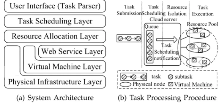
VERVIEW

The system architecture of our composite cloud service sys-tem is shown in Fig. 1a. A user request (a.k.a., a task) is made up of multiple subtasks connected in parallel or sequentially. Each subtask is an instance of an off-the-shelf service that has a very convenient interface (such API) to be called. Each whole task is expected to be completed as soon as possible under the constraint of its budget. Task scheduling is a key layer to coordinate the task priorities. Resource allocation layer is responsible for calculating the optimal resource frac-tion for the subtasks. Each physical host runs multiple VMs, on each of which are deployed with all of the off-the-shelf services (e.g., the libraries or programs that do the computa-tion). Each subtask will be executed on a VM, with an amount of virtual resource fraction tuned by the substrate VM moni-tor (VMM, a.k.a., hypervisor). Fault tolerance is beyond the scope of the paper, and we discuss this issue in [17] in details.

Each task is processed via a scheduling queue, as shown in Fig. 1b. Tasks are submitted continually over time, and each task submitted will be analyzed by a task

parser (in the user interface module), in order to predict

the subtask workloads based on input parameters. Sub-task’s workload can be characterized using {resource_ processing_ratesubtask_execution_length} based on his-torical traces or workload prediction approaches like poly-nomial regression method [18]. Our optimization model will compute the optimal resource vector of all subtasks for the task. And then, the unprocessed subtasks with no dependent preceding unprocessed subtasks will be put/ registered in a queue, waiting for the scheduling notifica-tion. Upon being notified, the hypervisor of the selected physical machine will launch a VM and perform the resource isolation to match optimization demand. The cor-responding service on the VM will be called using specific

input parameters, and the output will be cached in the VM, waiting for the notification of the data transmission for its succeeding subtask.

We adopt XEN’s credit scheduler [19] to perform the resource isolation among VMs on the same physical machine. With XEN [20], we can dynamically isolate some key resources (like CPU rate and network bandwidth) to suit the specific usage demands of different tasks. There are two key concepts in the credit scheduler, capacity and weight. Capacity specifies the upper limit on the CPU rate consum-able by a particular VM, and weight means a VM’s propor-tional-share credit. On a relatively free physical host, the CPU rate of a running VM is determined by its capacity. If there are over-many VMs running on a physical machine, the real CPU rates allocated for them are proportional to their weights. Both capacity and weight can be tuned at runtime.

3

P

ROBLEM

F

ORMULATION

Assuming there arentasks to be processed by the system, and they are denoted asti, where i¼1, 2,. . .; n. Each task

is made up of multiple subtasks connected in series or in parallel. We denote the subtasks of the tasktito betið1Þ,tið2Þ,

. . .,tiðmiÞ, wheremi refers to the number of subtasks in ti.

Such a formulation is generic enough such that any user request (or task) can be constructed by multiple nested com-posite services (or subtasks).

Task execution time is represented in different ways based on different intra-structure about subtask connection. For the sequential-mode task, its total execution time (or exe-cution length) can be denoted asT(ti)¼

Pmi

j¼1 l_iðjÞ

r_iðjÞ, whereliðjÞ

andriðjÞ are referred to as the workload of subtasktiðjÞand the compute resource allocated respectively. The workload here is evaluated by the number of instructions or data to read/write from/to disk, and the compute resource here means workload processing rate like CPU rate and disk I/O bandwidth. As for a parallel mode task (e.g., embarrassingly parallel application), its total execution length is equal to the longest execution time of its subtasks (or makespan). We will use execution time, execution length, response length, and wall-clock time interchangeably in the following text.

Each subtasktiðjÞwill call a particular service API, which

is associated with a service price (denoted aspiðjÞ). The

vice prices ($/unit) are determined by corresponding ser-vice makers in our model, since they are the ones who pay monthly resource leases to infrastructure-as-a-service (IaaS) providers (e.g., Amazon EC2 [21]). The total payment in executing a task ti on top of service layer is equal to

Pm_i

j¼1½riðjÞpiðjÞ. Each task is associated with a budget

(denoted asBðtiÞ) by its user in order to control its total

pay-ment. Hence, the problem of optimizing taskti’s execution

can be formulated as Formulas (1) and (2) (convex-optimi-zation problem) minTðtiÞ ¼ Pmi j¼1 l_iðjÞ r_iðjÞ; tiis in sequential mode maxj¼1mi l_iðjÞ r_iðjÞ ; tiis in parallel mode 8 < : (1) s:t: X m_i j¼1 ½riðjÞpiðjÞ BðtiÞ: (2)

There are two metrics to evaluate the system perfor-mance. One is RER of each task (defined in Formula (3))

RERðtiÞ ¼ t 0

is real response time

t0_is theoretically optimal length: (3) The RER is used to evaluate the execution performance for a particular task. The lower value the RER is, the higher exe-cution efficiency the corresponding task is processed in reality. A sequential-mode task’stheoretically optimal length

(TOL) is the sum of the theoretical execution time of each subtask based on the optimal resource allocation solution to the above problem (Formulas (1) and (2)), while a paral-lel-mode task’s TOL is equal to the largest theoretical sub-task execution time. The response time here indicates the whole wall-clock time from a task’s submission to its final completion. In general, the response time of a task includes subtask’s waiting time, overhead before subtask execution (e.g., on resource allocation or data transmission), subtask’s productive time, and processing overhead after execution. We try best to minimize the cost for each part.

The other metric is the fairness index of RER among all tasks (defined in Formula (4)), which is used to evaluate the fairness of the treatment in the system. Its value is ranged in [0, 1], and the bigger its value is, the higher fairness of the treatment is. Based on Formula (3), the fairness is also related to the different types of execution overheads. How to effectively coordinate the overheads among different tasks is a very challenging issue. This is mainly due to largely different task structure (i.e., the subtask’s workload and their connection way), task budget, and varied resource availability over time

fairnessðtiÞ ¼

Pn

i¼1RERðtiÞ 2

nPn_i¼1RER2ðtiÞ: (4) Our final objective is to minimize RER for each individ-ual task (or minimize the maximum RER) and maximize the overall fairness, especially in a competitive situation with over-many submitted tasks.

4

O

PTIMIZATION OF

S

YSTEM

P

ERFORMANCE

In order to optimize the entire QoS for each task, we need to minimize the time cost at each step in the course of its exe-cution. We study the best-fit solution with respect to three following facets, resource allocation, task scheduling, and minimization of overheads.

4.1 Optimized Resource Allocation with VMs

We first derive an optimal resource vector for each task (including parallel-mode task and sequential-mode task), subject to task structure and budget, in both petitive situation and competitive situation. In non-com-petitive situation, there are always available and adequate resources for task processing. As for an committed situation (or competitive situation), the over-all resources are over-committed such that the requested resource amounts succeed the de-facto resource amounts in the system. In this situation, we designed an adjust-able resource allocation method for maintaining the high performance and fairness.

4.1.1 Optimal Resource Allocation in Non-Competitive Situation

In a non-competitive situation (with unlimited available resource amounts), the resource fraction allocated to some task is mainly restricted by its user-set budget. Based on the target function (Formula (1)) and a constraint (Formula (2)), we analyze the two types of tasks (sequential-mode and parallel-mode) respectively.

Optimization of Sequential-Mode Task:

Theorem 1.If taskti is constructed in sequential mode,

ti’s optimal resource vector rrðtiÞ for minimizing

TðtiÞsubject to the constraint (2) is shown as Equa-tion (5), wherej¼1, 2,. . .; mi r_iðjÞ¼ ffiffiffiffiffiffiffiffiffiffiffiffiffiffiffi l_iðjÞ=:p_iðjÞ p Xmi k¼1 ffiffiffiffiffiffiffiffiffiffiffiffiffiffiffiffi liðkÞpiðkÞ q BðtiÞ: ₍₅₎ Proof.Since@2TðtiÞ @rj ¼2 liðjÞ r3 iðjÞ >0,T(ti) is convex with a

minimum extreme point. By combining the con-straint (2), we can get the Lagrangian function as Formula (6), where refers to the Lagrangian multiplier FðriÞ ¼X mi j¼1 liðjÞ riðjÞ þ BðtiÞ X mi j¼1 riðjÞpiðjÞ ! : (6) We derive Equation (7) via Lagrangian multiplier method rið1Þrið2Þ riðm_iÞ¼ ffiffiffiffiffiffiffi l_ið1Þ p_ið1Þ r : ffiffiffiffiffiffiffi l_ið2Þ p_ið2Þ r : : ffiffiffiffiffiffiffiffiffi l_iðmiÞ p_iðmiÞ r : (7)

In order to minimizeTðtiÞ, the optimal resource vectorrr_iðjÞshould use up all budgets (i.e., let the total payment be equal toBðtiÞ). Then, we can get

Equation (5). tu

As follows, we discuss the significance of Theo-rem 1 and how to split physical resources among dif-ferent tasks based on VM resource isolation in practice. According to Theorem 1, we can easily com-pute the optimal resource vector for any task based on its budget constraint. Specially,r_iðjÞis the theoreti-cally optimal resource vector (or processing rate) allocated to the subtasktiðjÞ, such that the total

wall-clock time of tasktican be minimized. That is, even

though there were more available resources com-pared to the valuer_iðjÞ, it would be useless for the tasktidue to its limited budget. In this situation, our

resource allocator will allocate the theoretically opti-mal resource fraction (Formula (5)) to each subtask’s resource capacity (such as maximum CPU rate).

Optimization of Parallel-Mode Task:

Theorem 2.If tasktiis constructed in the parallel mode,

ti’s optimal resource vector rrðtiÞ for minimizing

TðtiÞ subject to the constraint (2) is shown as Equa-tion (8), wherej¼1, 2,. . .; mi

r_iðjÞ¼Pm_iliðjÞ j¼1piðjÞliðjÞ

BðtiÞ: (8)

Proof.We just need to prove the optimal situation occurs if and only if all of subtask execution lengths are equal to each other. That is, the entire execution length of a parallel-mode task will be minimized if and only if Equation (9) holds

lið1Þ rið1Þ ¼lið2Þ rið2Þ ¼ ¼liðmiÞ riðmiÞ : (9)

In this situation, we can easily derive equation (8) by using up the user-preset budgetBðtiÞ, i.e., let-tingPmi

j¼1½riðjÞpiðjÞ ¼BðtiÞhold.

As follows, we use proof-by-contradiction method to prove that Equation (9) is a necessary condition of the optimal situation by contradic-tion. Let us suppose an optimal situation with minimized task wall-clock length occurs while Equation (9) does not hold. Without loss of gener-ality, we denote by tiðkÞ the subtask that has the

longest execution time (i.e., liðkÞ

r_iðkÞ), that is,

TðtiÞ ¼l_riðkÞ

iðkÞ. Since equation (9) does not hold, there must exist another subtasktiðjÞsuch that

l_iðjÞ riðjÞ<

l_iðkÞ riðkÞ. Obviously, we are able to add a small increment

~k to riðkÞ and decrease riðjÞ by ~j

correspond-ingly, such that the total payment is unchanged and the two subtasks’ wall-clock lengths become the same. That is, Equations (10) and (11) hold simultaneously riðjÞpiðjÞþriðjÞpiðkÞ¼ ðriðjÞDjÞpiðjÞþ ðriðjÞþDkÞpiðkÞ (10) liðjÞ riðjÞDj¼ liðkÞ riðkÞþDk : (11)

It is obvious that the new solution withDjand Dkgets the further reduced task wall-clock length,

which contradicts to our assumption that the pre-vious allocation is optimal. tu 4.1.2 Adjusted Resource Allocation to Adapt

to Competitive Situation

If the system runs in short supply, it is likely the total sum of their optimal resources (i.e., rðtiÞ) may succeed the total capacity of physical machines. At such a com-petitive situation, it is necessary to coordinate the priori-ties of the tasks in the resource consumption, such that none of tasks’ real execution lengths would be extended noticeably compared to its theatrically optimal execution length (i.e., minimizing RER(ti) for each task ti). In our

system, we improve the proportional-share model [22] with XEN’s credit scheduler by further enhancing resource fractions for short tasks.

Under XEN’s credit scheduler, each guest VM on the same physical machine will get its CPU rate that is

proportional to its weight.1 Suppose on a physical host (denoted as hi), ni scheduled subtasks are running on ni

stand-alone VMs separately (denoted vj, where j¼1, 2,

. . .ni). We denote the hosthi’s total compute capacity to beci

(e.g., eight cores), and the weights of theni subtasks to be

wðv1Þ, wðv2Þ, . . . , wðvniÞ. Then, the real resource fraction

(denoted byrðvjÞ) allocated to the VMvjcan be calculated by

Formula (12)

rðvjÞ ¼PnwiðvjÞ

k¼1wðvkÞ

ci: (12)

Now, the key question becomes how to determine the weight value for each running subtask (or VM) on a physi-cal machine, to adapt to the competitive situation. We devise a novel model, namely adjusted proportional-share

model (APSM), which further tunes the credits based on

task’s workload (or execution length). The design of APSM is based on the definition of RER: a large value of RER tends to appear with a short task. This is mainly due to the fact that the overheads (such as data transmission cost, VMM operation cost) in the whole wall-clock time are often rela-tively constant regardless of the total task workload. That is, based on RER’s definition, short task’s RER is more sensi-tive to the execution overheads than that of a long one. Hence, we make short tasks tend to get more resource frac-tions than their theoretically optimal vector (i.e.,r_iðjÞ). There are two alternative ways to realize this effect.

Absolute mode. For this mode, we use a threshold

(denoted ast) to split running tasks into two catego-ries, short tasks (workloadt) and long tasks (work-load>t). Three values oft are investigated in our experiments: 500, 1,000, or 2,000, which corresponds to 5, 10 or 20 seconds when running a task on a single core. We assign as much resource as possible to short tasks, while keeping the long tasks’ resource fractions unchanged. Task length is evaluated in terms of its workload to process. In practice, it can be estimated based on the workload characterization over history or workload prediction method like [18]. In our design based on the absolute mode, short tasks’ cred-its will be set to 800 (i.e., eight cores), implying the full computational power. For example, if there is only one short running task on a host, it will be assigned with full resources (eight cores) for its com-putation. If there are more running tasks, they will be allocated according to PSM, while short tasks will be probably assigned with more resource fractions.

Relative mode. Our intuitive idea is adopting a

proportional-share model on most of the middle-size-tasks such that their resource fractions received are proportional to their theoretically optimal resource amounts (r_iðjÞ). Meanwhile, we enhance the credits of the subtasks whose corresponding tasks are relatively short and decrease the credits of the ones with long tasks. That is, we give some extra credits to short tasks to enhance their resource con-sumption priority. Suppose on a physical machine

is runningdsubtasks (belonging to different tasks), which are denoted ast_1ðx₁Þ,t2ðx₂Þ,. . .,tdðxdÞ, where

xi ¼1, 2,. . ., ormi. Then,wðtiðjÞÞwill be determined by either Formula (13) or Formula (14), based on dif-ferent proportional-share credits (either task’s workload or task’s TOL). Hence, the relative mode based APSM (abbreviated as RAPSM) has two dif-ferent types, workload-based APSM (abbreviated as RAPSM(W)) and TOL-based APSM (abbreviated as RAPSM(T)) wðtiðjÞÞ ¼ hr_iðjÞ lia r_iðjÞ a< lib 1 hriðjÞ li>b 8 < : (13) wðtiðjÞÞ ¼ hr_iðjÞ TðtiÞ a r_iðjÞ a < TðtiÞ b 1 hriðjÞ TðtiÞ > b: 8 > < > : (14)

The weight values in our design (Formula (13)) are determined by four parts, the extension coefficient (h), theoretically optimal resource fraction (r_iðjÞ), the threshold valueato determine short tasks, and the threshold value b to determine long tasks. Obvi-ously, the value of h is supposed to be always greater than 1. In reality, tuning h’s value could adjust the extension degree for short/long tasks. Changing the values ofaandbcould tune the num-ber of the short/long tasks. That is, by adjusting these values dynamically, we could optimize the overall system performance to adapt to different contention states. Specific values suggested in prac-tice will be discussed with our experimental results. In practice, one could use either of the above two modes or both of them, to adjust the resource allocation to adapt to the competitive situation.

4.2 Best-Suited Task Scheduling Policy

In a competitive situation where over-many tasks are sub-mitted to the system, it is necessary to queue some tasks that cannot find the qualified resources temporarily. The queue will be checked as soon as some new resources are released or new tasks are submitted. As multiple hosts are available for the task (e.g., there are still available CPU rates non-allocated on the host), the most powerful one with the largest availability will be selected as the execution host. A key question is how to select the waiting tasks based on their demands, such that the overall execution performance and the fairness can both be optimized.

Based on the two-fold objective that aims to minimize the RER and maximize the fairness meanwhile, we investigate the best-fit scheduling policy for both sequential-mode tasks and parallel-mode tasks. We propose that (1) the best-fit queuing policy for the sequential-mode tasks is lightest-workload-first policy, which assigns the highest scheduling priority to the shortest task that has the least workload amount to process; (2) the best-fit policy for parallel-mode tasks is adopting LWF and longest-subtask-first (LSTF) 1. Weight-setting command is “xm sched-credit -d VM -wweight”.

together. In addition, we also evaluate many other queuing policies for comparison, including FCFS, SOLF, SPF, SSTF, and so on. We describe all the task-selection policies below.

FCFS. FCFS schedules the subtasks based on their arrival order. The first arrival one in the queue will be scheduled as long as there are available resources to use. This is the most basic policy, which is the easi-est to implement. However, it does not take into account the variation of task features, such as task structure, task workload, thus the performance and fairness will be significantly restricted.

Lightest-Workload-First. LWF schedules the subtasks

based on the predicted workload of their correspond-ing tasks (a.k.a., jobs). Task’s workload is defined as the execution length estimated based on a standard process rate (such as single-core CPU rate). In the waiting queue, the subtask whose corresponding task has lighter workload will be scheduled with a higher priority. In our Cloud system that aims to min-imize the RER and maxmin-imize the fairness meanwhile, LWF obviously possesses a prominent advantage. Note that various tasks’ TOLs are different due to their different budget constraints and workloads, while tasks’ execution overheads tend to be constant because of usually stable memory size consumed over time. In addition, the tasks with lighter work-loads tend to be with smaller TOLs, based on the defi-nition ofTðtiÞ. Hence, according to the definition of

RER, the tasks with lighter workloads (i.e., shorter jobs) are supposed to be more sensitive to their execu-tion overheads, which means that they should be associated with higher priorities.

SOLF. SOLF is designed based on such an intui-tion: in order to minimize RER of a task, we can only minimize the task’s real execution length because its theoretically optimal length (TOL) is a fixed constant based on its intrinsic structure and budget. Since tasks’ TOLs are different due to their heterogeneous structures, workloads, and budgets, the execution overheads will impact their RERs to different extents. Suppose there were two tasks whose TOLs are 30 and 300 seconds respectively and their execution overheads are both 10 seconds. Even though the sums of their subtask execution lengths were right the optimal values (30 and 300 seconds), their RERs would be largely different:

30þ10

30 versus 300300þ10. In other words, the tasks with

shorter TOLs are supposed to be scheduled with higher priorities, for minimizing the discrepancy among tasks’ RERs.

SPF. SPF is designed for sequential-mode tasks, based on task’s real execution progress compared to its overall workload or TOL. The tasks with the slow-est progress will have the highslow-est scheduling priori-ties. The execution progress can be defined based on either the workload processed or the wall-clock time passed. They are called workload progress(WP) and

time process(TP) respectively, and they are defined in Formulas (15) and (16) respectively. In the two for-mulas,drefers to the number of completed subtasks,

li¼ Pmi j¼1liðjÞ, and TOLðtiÞ ¼ Pmi j¼1 l_iðjÞ r iðjÞ. SPF means that the smaller value of ti’s WPðtiÞ or TPðtiÞ, the

higherti’s priority would be. For example, ifti is a

newly submitted task, its workload processed must be 0 (ord= 0), thenWPðtiÞwould be equal to 0, indi-catingtiis with the slowest process

WPðtiÞ ¼

Pd

j¼1liðdÞ

li ;

(15) TPðtiÞ ¼wallclock time since t0is submission

TOLðtiÞ : (16)

Based on the two different definitions, the SPF can be split into two types, namely slowest-workload-prog-ress-first (SWPF) and slowest-time-progslowest-workload-prog-ress-first (STPF) respectively. We evaluated both of them in our experiment.

SSTF. SSTF selects the shortest subtask waiting in the queue. The shortest subtask is defined as the subtask (in the waiting queue) which has the minimal work-load amount estimated based on single-core compu-tation. As a subtask is completed, there must be some new resources released for other tasks, which means that a new waiting subtask will then be scheduled if the queue is non-empty. Obviously, SSTF will result in the shortest waiting time to all the subtasks/tasks on average. In fact, since we select the “best” resource in the task scheduling, the eventual scheduling effect of SSTF will make the short subtasks be executed as soon as possible. Hence, this policy is exactly the same asmin-minpolicy [15], which has been effective in Grid workflow scheduling. However, our experi-ments validate that SSTF is not the best-suited sched-uling policy in our Cloud system.

LWFþLSTF. We can also combine different individ-ual policies to generate a new scheduling policy. In our system, LWFþLSTF is devised for parallel-mode task, whose total execution length is deter-mined by its longest subtask execution length (i.e., makespan), thus the subtasks with heavier work-loads in the same task will have higher priority to schedule. On the other hand, in order to minimize the overall waiting time, all of tasks will be sched-uled based on lightest workload first. LWFþLSTF means that the subtasks whose task has the lightest workload will have the highest priority and the sub-tasks belonging to the same task will be scheduled based on longest subtask first. In addition, we also implement LWFþSSTF for comparison.

4.3 Minimization of Processing Overheads

In our system, in addition to the waiting time and execution time of subtasks, there are three more overheads which need also to be counted in the whole response time, VM resource isolation cost, data transmission cost between sub-tasks, and VM’s default restoring cost. Our cost-minimization strategy is performing the data transmission and VMM operations concurrently, based on the characterization of their costs. We also assign extra amount of resources to super-short tasks (e.g., the tasks with TOL2 seconds) in order to

mitigate the impact of the overhead to their executions. Spe-cifically, we run them directly on VMs without any credit-tuning operation. Otherwise, the credit-credit-tuning effect may work on another subtask instead of the current subtask, due to the inevitable delay (about 0.3 seconds) of the credit-tuning command. Details can be found in our corresponding conference paper [24].

5

P

ERFORMANCE

E

VALUATION

5.1 Experimental Setting

We implement a cloud composite service prototype that can help solve complex matrix problems, each of which is allowed to contain a series of nested or parallel matrix com-putations. For an example of nested matrix computation, a user may submit a request likeSolve((AmnAnm)k,Bmm),

which can be split into three steps (or subtasks): (1) matrix-product (a.k.a., matrix-matrix multiply): Cmm¼Amn

Anm; (2) matrix-power:Dmm¼Cmkm; (3) calculating least

squares solution ofDX¼B:Solve(Dmm,Bmm).

In our experiment, we make use of ParallelColt [25] to perform the math computations, each consisting of a set of matrix computations. ParallelColt [25] is such a library that can effectively calculate complex matrix computations, such as matrix-matrix multiply and matrix decomposition, in parallel (with multiple threads) based on symmetric multi-ple processor (SMP) model.

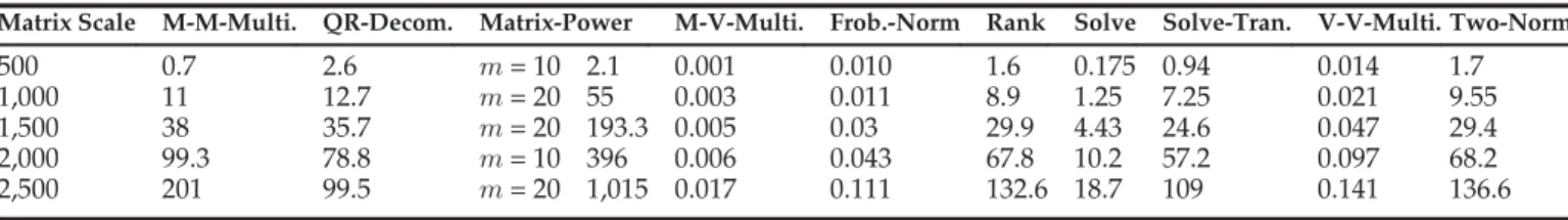
There are totally 10 different matrix computations (such as matrix-product, matrix-decomposition, etc.) as shown in Table 1. We carefully characterize the single-core execu-tion length (or workload) for each of them, and find that each matrix computation has its own execution type. For example, matrix-product and matrix-power are typical computation-intensive services, while rank and two-norm computation should be memory-intensive or I/O-bound ones when matrix scale is large. Hence, each sequential-mode task that is made up of multiple different matrix computations in series can be considered complex applica-tions with execution types varied over time.

In each test, we randomly generate a number of user requests, each of which is composed of 5 15 sub-tasks (or matrix computation services). Such a simulation is non-trivial since each emulated matrix has to be compatible for each matrix computation (e.g., two matrices in a matrix-product must be in the form ofAmnandBnprespectively).

Among the 10 matrix-computation services, three services are implemented as multiple-threaded programs, including matrix-matrix multiply, QR-decomposition, matrix-power, hence their computation can get an approximate-linear speedup when allocated multiple processors. The other seven matrix operation services are implemented using

single thread, thus they cannot get speedup when being allocated with more than one processor. Hence, we set the capacity of any subtask performing a single-threaded ser-vice to be single-core rate, or less when its theoretically opti-mal resource to allocate is less than one core.

In our experiment, we are assigned with eight physical nodes to use from the most powerful cluster at HongKong (namely Gideon-II [23]), and each node owns two quad-core Xeon CPU E5540 (i.e., eight processors per node) and 16 GB memory size. There are 56 VM-images (centos 5.2) maintained by Network File System (NFS), so 56 VMs (seven VMs per node) will be generated at the bootstrap. XEN 4.0 [20] serves as the hypervisor on each node and dynamically allocates various CPU rates to the VMs at run-time using the credit scheduler.

We will evaluate different queuing policies and resource allocation schemes under different competitive situations with different numbers (4-24) of tasks simultaneously. Table 2 lists the candidate key parameters we investigated in our evaluation. Note that the measurement unit ofhand

bfor RAPSM(T) is second, while the measurement unit for RAPSM(W) is seconds100, because a single core’s proc-essing ability is represented as 100 according to XEN’s credit scheduler [19], [20].

5.2 Experimental Results

5.2.1 Demonstration of Resource Contention Degrees We first characterize the various contention degrees with different number of tasks submitted. The contention degree is evaluated via two metrics, allocate-request ratio

(abbreviated as ARR) and queue length (abbreviated as

QL). System’s ARR at a time point is defined as the ratio of the total allocated resource amount to the total amount requested by subtasks at that moment. QL at a time point is defined as the total number of subtasks in the waiting list at that moment. There are four test-cases each of which uses different number of tasks (4, 8, 16, and 24) submitted. The four test-cases correspond to different contention degrees.

TABLE 1

Workloads (Single-Core Execution Length) of 10 Matrix Computations (Seconds)

Matrix Scale M-M-Multi. QR-Decom. Matrix-Power M-V-Multi. Frob.-Norm Rank Solve Solve-Tran. V-V-Multi. Two-Norm

500 0.7 2.6 m= 10 2.1 0.001 0.010 1.6 0.175 0.94 0.014 1.7 1,000 11 12.7 m= 20 55 0.003 0.011 8.9 1.25 7.25 0.021 9.55 1,500 38 35.7 m= 20 193.3 0.005 0.03 29.9 4.43 24.6 0.047 29.4 2,000 99.3 78.8 m= 10 396 0.006 0.043 67.8 10.2 57.2 0.097 68.2 2,500 201 99.5 m= 20 1,015 0.017 0.111 132.6 18.7 109 0.141 136.6 TABLE 2

Candidate Key Parameters

Parameter Value

threshold of short task length (seconds) 5, 10, 20

h 1.25, 1.5, 1.75, 2

aw.r.t. RAPSM(T) (seconds) 5, 10, 20

bw.r.t. RAPSM(T) (seconds) 100, 200, 300

aw.r.t. RAPSM(W) (seconds100) 500, 1,000, 2,000

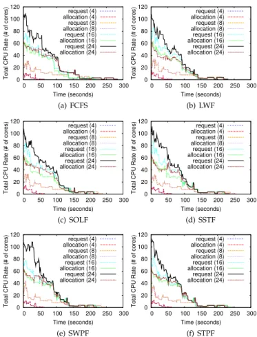
Fig. 2 shows the summed resource amount allocated and the summed amount requested over time under different competitive situations, with exactly the same experimental settings except for different scheduling policies. The num-bers enclosed in parentheses indicate the number of tasks submitted.

We find that with the same number of submitted tasks, ARR exhibits similarly with different scheduling policies. The resource amount allocated can always meet the resource amount requested (i.e., ARR keeps one and two curves overlap in the figure) when there are a small number (4 or 8) of tasks submitted, regardless of the scheduling poli-cies. This confirms our resource allocation scheme can guar-antee the service level in the non-competitive situation. As the system runs with over-many tasks (such as 16 and 24) submitted, there would appear a prominent gap between the resource allocation curve and the resource request curve. This clearly indicates a competitive situation. For

instance, when 24 tasks are submitted simultaneously, ARR stays around 1/2 during the first 50 seconds. It is also worth noting that the longest task execution length under FCFS is remarkably longer than that under LWF (about 280 seconds versus about 240 seconds). This implies scheduling policy is essential to the performance of Cloud system.

Fig. 3 presents that the QL increases with the number of tasks submitted. It is worth noticing that QL under different scheduling policies exhibits quite different. In the duration with high competition (the first 50 seconds in the test), SSTF and LWF both lead to small number of waiting tasks (about 5-6 and 6-7 respectively). By contrast, under SOLF, SWPF, or STPF, QL is much longer (about 10-12 waiting tasks on average), implying a longer waiting time.

5.2.2 Investigation of Best-Suited Strategy

We explore the best-suited scheduling policy and resource allocation scheme, in a competitive situation with 24 tasks (allocate-request ratio 1₂ for the first 50 seconds). The investigation is for sequential-mode tasks and parallel-mode tasks respectively.

A. Best-suited strategy for sequential-mode tasks. Fig. 4 shows the distribution (cumulative distribution function) of RER in the competitive situation, with different scheduling policies

Fig. 2. Allocation versus request with different contention degrees.

Fig. 3. Queue lengths with different scheduling policies.

Fig. 4. Distribution of RER in a competitive situation.

TABLE 3

Statistics of RER in a Competitive Situation with Sequential-Mode Tasks

strategy min. avg. max. fairness

FCFSþPSM 0.712 3.919 22.706 0.352 FCFSþRAPSM(T) 0.718 4.042 23.763 0.351 FCFSþRAPSM(W) 0.720 4.137 24.717 0.348 LWFþPSM 0.720 2.106 8.202 0.628 LWFþRAPSM(T) 0.719 2.172 8.659 0.603 LWFþRAPSM(W) 0.723 2.122 7.937 0.630 SOLFþPSM 0.736 2.979 13.473 0.506 SOLFþRAPSM(T) 0.745 3.252 14.625 0.527 SOLFþRAPSM(W) 0.738 3.230 14.380 0.526 SSTFþPSM 0.791 2.068 8.263 0.591 SSTFþRAPSM(T) 0.769 2.169 9.024 0.566 SSTFþRAPSM(W) 0.770 2.126 8.768 0.579 SWPFþPSM 0.713 6.167 58.691 0.209 SWPFþRAPSM(T) 0.726 6.532 62.332 0.208 SWPFþRAPSM(W) 0.718 6.477 61.794 0.208 STPFþPSM 0.723 3.176 16.398 0.465 STPFþRAPSM(T) 0.723 3.208 15.831 0.475 STPFþRAPSM(W) 0.722 3.188 15.399 0.485

used for the sequential-mode tasks. For each policy, we ran the experiments with all the possible combinations of param-eters shown in Table 2, and then compute the distribution. It is clearly observed that the RERs under LWF and SSTF are much smaller than those under other policies. By contrast, The two worst policies are SWPF and SOLF, whose maxi-mum RERs are even up to 105 and 55 respectively. The main reason is that LWF and SSTF lead to much shorter waiting time than SWPF and SOLF, according to Fig. 3.

In addition to task scheduling policy, we also investigate the best-fit resource allocation scheme. In Table 3, we show the statistics of RER with various solutions, by combining different scheduling policies and resource allocation schemes. We evaluate each solution with all of different combinations of parameters (includingt,h,a, and b) and compute the statistics (including minimum, average, maxi-mum, and fairness value).

Through Table 3, we observe that LWF and SSTF result in the lowest RERs on average and at the worst case, which is consistent with the distribution of RER as shown in Fig. 4. They improve the performance by3:919

2:1 1¼86:6%, as

com-pared to FCFS policy. It is also observed that relative mode based adjusted PSM (RAPSM) may not further reduce the RER as expected. This means that RAPSM cannot directly improve the execution performance without absolute mode based adjusted PSM (AAPSM). Later, we will show in Section 5.2.3 that the solutions with AAPSM can signifi-cantly reduce RER, in comparison to the RAPSM.

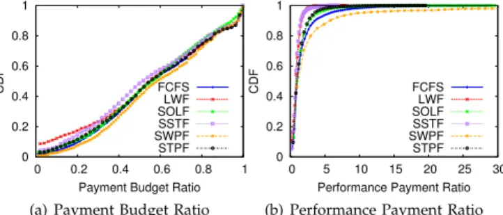
We also show the distributions of payment budget ratio (PBR) and performance payment ratio (PPR) in Fig. 5. Through Fig. 5a, we observe that all of tasks’ payments are guaranteed below their budgets. This is due to the strict payment-by-reserve model (Formula (2) and Theorem 1) we always followed in our design. Through Fig. 5b, it is also observed that PPR exhibits similarly to RER. For example, two best scheduling policies are also LWF and SSTF. Their mean PPRs are 0.874 and 0.883 respectively; their maximum PPRs are 8.176 and 6.92 respectively. Apparently, if we do not take into account the difference of adjusted resource allocation scheme but task scheduling policy, SSTF outper-forms others prominently due to its shortest waiting time on average.

B. Best-suited strategy for parallel-mode tasks. We also

explore the best-suited scheduling strategy with respect to the parallel-mode tasks. Table 4 presents different mini-mum/average/maximum/fairness values of RER when scheduling parallel-mode tasks by different policies, includ-ing FCFS, LWF, SSTF, etc. Note that SPF is not included because all of subtasks in a task will be executed in parallel,

so that it is meaningless to characterize the processing prog-ress, unlike the situation with sequential-mode tasks.

Each test is conducted with 24 tasks, and each task ran-domly contains 5-15 parallel matrix-power computation subtasks. Since there are only eight physical execution nodes, so this is a competitive situation where some tasks have to be queued for scheduling. In this experiment, we also implement heaviest workload first (HWF) combined with longest (shortest) subtask first for comparison.

Based on Table 4, we can observe that LWF always leads to a fairly high scheduling performance. For example, when only adopting LWF, the average RER is about 1.30, which is lower than that of FCFS by1:51:3

1:5 ¼13.3%, and lower than

SSTF by2:091:3

2:09 ¼37.8%. Adopting the LWFþLSTF (i.e., the

combination of LWF and SSTF) can minimize the maximum RER to be 3.58, which is lower than other strategies by 3.8 percent (LWF)—51.6 percent (HWFþSSTF).

The key reason why LWF exhibits much better results is that LWF schedules the shortest tasks with highest priority, suffersing the least overall waiting time. In particular, not only can LWFþLSTF minimize the maximum ERE, but it can also lead to the highest fairness (up to 0.96), which means a fairly high stability of the LWFþLSTF policy. This is because each task is a parallel-mode task, such that longest subtask first can effectively minimize the makespan for each task, optimizing the execution performance for a particular task. 5.2.3 Exploration of Best-Fit Parameters

In this section, we comprehensively compare various solu-tions with different scheduling policies and adjusted resource allocation schemes with different parameters shown in Table 2, in a both competitive situation (i.e., AAR is about 1/2) and non-competitive situation (i.e., AAR approaches 1). We find that the adjusted resource allocation scheme could effectively improve the execution perfor-mance (RER and PPR), only when combining it with the Absolute Mode based Adjusted PSM (AAPSM).

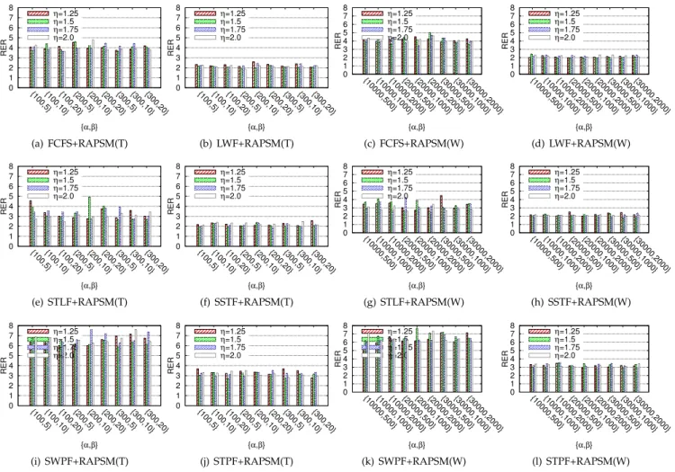
A. Evaluation in a competitive situation. Fig. 6 shows the

RER of various solutions with different parameters, includ-ingh,a, andb. It is observed that various policies with dif-ferent choices of the three parameters lead to difdif-ferent results. The smallest RER (best result) is 1.77, when adopt-ing SSTFþRAPSM(W) and h, a, and b being set to 1.75, 30,000, and 1,000. The largest RER (worst case) is 7.69, when adopting SWPFþRAPSM(W) andh,a, and b being set to 1.5, 20,000, and 1,000. We also find that different selections of the three parameters may affect the performance

Fig. 5. Distribution of PBR and PPR in a competitive situation.

TABLE 4

Statistics of RER in a Competitive Situation with Parallel-Mode Tasks

strategy min. avg. max. fairness

FCFS 2.75 1.50 4.97 0.89 LWF 2.25 1.30 3.72 0.92 HWF 3.04 1.45 6.25 0.86 SSTF 3.37 2.09 4.94 0.96 LWFþLSTF 2.34 1.57 3.58 0.96 LWFþSSTF 2.27 1.35 3.79 0.94 HWFþLSTF 3.20 1.43 6.88 0.81 HWFþSSTF 3.20 1.38 7.39 0.82

prominently for a few solutions like STLFþRAPSM(T) and STLFþRAPSM(W). However, they would not impact RER clearly in most cases. From Figs. 6b 6d, 6f and 6h, it is observed that with different parameters, the RERs under both LWF and SSTF are within [1.85, 2.31].

In our experiments, the most interesting and valuable finding is that the AAPSM with different short task length thresholds (t) will result in quite different results, which we show in Tables 5, 6 and 7. These three tables present the three key indicators, average RER, maximum

Fig. 6. Average RER of various solutions with different parameters.

TABLE 5

Mean RER under Various Solutions with Differenttandh

strategy t h¼1.25 h¼$1.5 h¼1.75 h¼2 FCFS 5 4.050 4.142 4.131 4.054 10 4.122 3.952 3.924 3.845 20 4.121 4.196 4.139 4.296 LWF 5 2.071 2.090 2.169 2.138 10 2.268 2.133 2.179 2.152 20 2.194 1.935 2.194 2.218 SOLF 5 3.316 3.321 3.552 3.102 10 3.241 3.382 2.989 2.783 20 3.375 3.324 3.305 3.039 SSTF 5 2.111 2.072 2.275 2.147 10 2.202 2.171 1.980 2.172 20 2.322 1.968 2.092 2.205 STPF 5 3.265 3.011 3.271 3.119 10 3.296 3.024 3.152 3.132 20 3.200 3.326 3.318 3.244 SWPF 5 6.169 6.371 6.339 6.322 10 6.271 6.353 6.446 6.659 20 6.784 6.763 6.730 6.635 TABLE 6

Max. RER under Various Solutions with Differenttandh

strategy t h¼1.25 h¼1.5 h¼1.75 h¼2 FCFS 5 23.392 25.733 24.742 24.470 10 24.184 22.397 22.633 23.192 20 24.204 25.258 24.391 25.313 LWF 5 9.164 7.826 8.543 8.323 10 10.323 7.681 9.136 9.104 20 8.106 5.539 6.962 8.812 SOLF 5 13.294 15.885 15.743 13.255 10 12.735 18.719 13.939 10.325 20 17.070 15.642 13.379 13.394 SSTF 5 8.091 7.931 9.276 9.803 10 10.245 8.376 7.224 11.199 20 11.418 6.432 6.706 9.650 STPF 5 16.456 15.545 17.642 15.232 10 16.925 14.797 15.892 14.710 20 13.978 15.596 16.250 14.853 SWPF 5 58.467 61.647 60.266 59.044 10 59.351 60.199 61.241 64.286 20 65.142 64.887 64.769 63.326

RER, and fairness index of RER, when adopting various solutions with different values of t and h. In our evalua-tion, we compute the average value for each of the three indicators, by traversing all of the remaining parameters, including a and b. Accordingly, the values shown in three tables can be deemed relatively stable mathematical expectation.

Through Table 5, we clearly observe that LWF and SSTF significantly outperforms other solutions, w.r.t. the mean values of RER. The mean values of RER under the two solu-tions can be restricted down to 1.935 and 1.968 respectively, when short task length threshold is set to 20 seconds. The mean value of RER under FCFS is about 4, which is about twice as large as that of LWF or SSTF. The worst situation occurs when adopting SWPFþRAPSM(W) and setting t to 20. In this situation, the mean value of RER is even up to 6.784, which is worse than LWF(t¼20) by 6:7841:935

1:935 ¼

250.6%. The reason whyt¼20is often better thant¼5is that the former assigns more resources to short tasks at run-time, significantly reducing the waiting cost in the system. However,t¼20is not always better thant¼5 ort¼10, in that the resource allocation is also related to other parame-ters likeh. That is, ifhis set to 2, thent¼20 will lead to an over-adjusted resource allocation situation, which exhibits worst results thant= 10.

Through Table 6, it is observed that that LWF and SSTF significantly outperforms other solutions, w.r.t. the maxi-mum values of RER (i.e., the worst case for each solution). In absolute terms, the expected value of the worst RER when adopting LWF witht¼20 is about 5.539, and SSTF’s is about 6.432, which is worse than LWF by 6:432

5:5391¼

16.1%. The worst case among all solutions happens when using SWPFþRAPSM(W), and the expected value of the worst RER is even up to 64.887, which is about 11.7 times as large as that of LWF (t¼20). The expected value of the worst RER under FCFS is about 23, which is about four times as large as that of LWF.

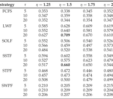
Table 7 shows the fairness of RER with different solu-tions. We find that the best result is adopting LWF witht and h being set to 20 and 1.5, and the expected fairness value is up to 0.709, which is better than the second best solution (SSTF, t¼20, h¼1.5) by about 0:7090:66

0:66 ¼7:4%.

From the three tables, we can conclude that LWF (t¼20,h¼1.5) is the best choice in the competitive situa-tion with AAR2.

In Fig. 7, we further investigate the performance (on minimum value, average value, and maximum value of RER) with more comprehensive combinations of parame-ters, by taking into account scheduling policy, AAPSM and RAPSM together. We find that LWF and SSTF result in best results when their short task length thresholds (t) are set to 20 and 10 seconds respectively. So, we just make the comparison in these two situations. It is observed that the mean values of RER of LWFþAAPSMþRAPSM(T) and LWFþAAPSMþRAPSM(W) (t¼20) can be down to 1.64 and 1.67 respectively, and their values of {a, b} are {300, 20} and {10,000, 2,000} respectively. In addition, the maxi-mum value of RER under LWFþAAPSMþRAPSM(T) (t¼

20) is about 3.9, which is the best result as we observed.

B. Evaluation in a non-competitive situation. For the non-competitive situation, there are eight tasks submitted and AAR is about 1 in the first 50 seconds. We compare the exe-cution performance (i.e., RER) when assigning different val-ues toh,a, andbin a non-competitive situation. For each set of parameters, we perform 144 tests, based on various task scheduling policies and different values of threshold of short task length (i.e., t), and then compute the CDF for each set of parameters, as shown in Fig. 8.

Through Fig. 8, it is observed that various assignments on the set of parameters result in different execution perfor-mance. For RAPSM(T) and RAPSM(W), {a¼200 s,b¼5 s} and {a¼20000,b¼500} often serve as the best assignment of the parameters respectively, regardless ofh’s value. For example, Fig. 8d shows that whenh is set to 2.0, {a¼200 seconds,b¼5 seconds} is better than other choices by [3.8, 7.1 percent]. In addition, we can also observe a relatively high instability in the other assignments of parameters. For

TABLE 7

Fairness of RER under Various Solutions with Differentt&h

strategy t h¼1.25 h¼1.5 h¼1.75 h¼2 FCFS 5 0.353 0.338 0.345 0.352 10 0.347 0.359 0.358 0.348 20 0.352 0.344 0.354 0.347 LWF 5 0.585 0.628 0.609 0.619 10 0.552 0.640 0.581 0.579 20 0.627 0.709 0.670 0.610 SOLF 5 0.552 0.506 0.540 0.526 10 0.566 0.459 0.497 0.573 20 0.484 0.520 0.538 0.541 SSTF 5 0.594 0.602 0.558 0.549 10 0.527 0.575 0.623 0.479 20 0.517 0.660 0.650 0.544 STPF 5 0.468 0.472 0.446 0.480 10 0.457 0.473 0.474 0.494 20 0.508 0.500 0.479 0.499 SWPF 5 0.210 0.205 0.209 0.215 10 0.210 0.209 0.209 0.204 20 0.206 0.207 0.206 0.208

instance, with RAPSM(T), {a¼100 seconds, b¼20 sec-onds} exhibits good results in Fig. 8c (h¼1.75), but bad results in Fig. 8 (h¼2.0); Using RAPSM(W) with {a¼10,000,b¼2,000}, about 93 percent of tasks’ RERs are below 1 when setting h to 1.75, while the corresponding ratio is only 86 percent when settingetato 2.0.

6

R

ELATED

W

ORK

Although job scheduling problem [26] in Grid computing [27] has been extensively studied for years, most of them (such as [28], [29]) are not suited for our cloud composite service processing environment. Grid jobs are often with long execution length, while Cloud tasks are often short based on [13]. Hence, task’s response time will be more eas-ily degraded by scheduling/execution overheads (such as waiting time and data transmission cost) in Cloud environ-ment than in Grid environenviron-ment. That is, the overheads in Cloud environment should be treated more carefully.

Recently, many new scheduling methods are proposed for different Cloud systems. Zaharia et al. [30] designed a task scheduling method to improve the performance of Hadoop [31] for a heterogeneous environment (such as a pool of VMs each being customized with different abilities). Unlike the FCFS policy and speculative execution model originally used in Hadoop, they designed a so-called lon-gest approximate time to end (LATE) policy, that assigns higher priorities to the jobs with longer remaining execution lengths. Their intuition is maximizing the opportunity for a speculative copy to overtake the original and reduce job’s response time. Isard et al. [32] proposed a fair scheduling policy (namely Quincy) for a high performance compute system with virtual machines, in order to maximize the scheduling fairness and minimize the data transmission cost meanwhile. Compared to these works, our Cloud sys-tem works with a strict payment model, under which the optimal resource allocation for each task can be computed based on convex optimization theory. Mao et al. [33], [34] proposed a solution by combining dynamic scheduling and EDF strategy, to minimize user payment and meet

application deadlines meanwhile. Whereas, they overlook the competitive situation by assuming the resource pool is always adequate and users have unlimited budgets. Many of other methods like Genetic algorithms [35] and Simulated Annealing algorithm [36], often overlooked the execution overheads in VM operation or data transmission, and per-formed the evaluation through simulation.

In addition to scheduling model, many Cloud manage-ment researchers focus on the optimization of resource assignment. Unlike Grid systems whose compute nodes are exclusively consumed by jobs, the resource allocation in Cloud systems are able to be refined by leveraging VM resource isolation technology. Stillwell et al. [37] exploited how to optimize the resource allocation for service hosting on a heterogeneous distributed platform. Their research is formalized as a mixed integer linear program (MILP) prob-lem and treated as a rational LP probprob-lem instead, also with fundamental theoretical analysis based on estimate errors. In comparison to their work, we intensively exploit the best-suited scheduling policy and resource allocation scheme for the competitive situation. We also take into account user pay-ment requirepay-ment, and evaluate our solution on a real-VM-deployment environment which needs to tackle more practi-cal technipracti-cal issues like minimization of various execution overheads. Meng et al. [38] analyzed VM-pairs’ compatibil-ity in terms of the forecasted workload and estimated VM sizes. SnowFlock [39] is another interesting technology that allows any VM to be quickly cloned (similar to UNIX process fork) such that the resource allocation would be automati-cally refined at runtime. Kuribayashi [40] also proposed a resource allocation method for Cloud computing environ-ments especially based on divisible resources. BlobCR [41] aims to optimize the performance of HPC applications on IaaS clouds at system level, by improving the robustness of running virtual machines using virtual disk image snap-shots. In comparison, our work focuses on the theoretical optimization of performance when system runs in short sup-ply and corresponding implementation issues at the applica-tion level.

7

C

ONCLUSION AND

F

UTURE

W

ORK

In this paper, we designed and implemented a loosely-coupled Cloud system with web services deployed on multiple VMs, aiming to improve the QoS of each user request and maximize fairness of treatment at runtime. Our contribution is three-fold: (1) we studied the best-suited task scheduling policy with VMs; (2) we explored an optimal resource allocation scheme and an adjusted strategy to suit the competitive situation; (3) the processing overhead is minimized in our design. Based on our experi-ments, we summarize the following lessons.

We confirm that the best scheduling policy of scheduling sequential-mode tasks in the competi-tive situations, is either lightest-workload-first or SSTF. Each of them improves the performance by about 86 percent compared to FCFS. As for the parallel-mode tasks, the best-fit policy is combin-ing LWF and longest subtask first, and the aver-age RER is lower than other solutions by 3.8-51.6 percent.

For a competitive situation, the best solution is com-bining lightest-workload-first with AAPSM and RAPSM (in absolute terms, LWFþAAPSMþRAPSM with short task length threshold and extension coef-ficient being set to 20 seconds and 1.5 respectively). It outperforms other solutions in the competitive sit-uation, by 16þ% w.r.t. the worst-case response time. The fairness under this solution is about 0.709, which is higher than that of the second best solution (SSTFþAAPSMþRAPSM) by7:4þ%.

For a non-competitive situation, {a¼200 seconds,

b¼5 seconds} serves as the best assignment of the parameters, regardless of the threshold value of set-ting the short task length (h).

In the future, we plan to further exploit an adaptive solu-tion that can dynamically optimize the performance in both competitive and non-competitive situations. We also plan to improve the ability of fault tolerance and resilience in our cloud system.

A

CKNOWLEDGMENTS

This work was made by the ANR project Clouds@home (ANR-09-JCJC-0056-01), also supported by the U.S. Depart-ment of Energy, Office of Science, under Contract DE-AC02-06CH11357, and also in part by HKU 716712E.

R

EFERENCES

[1] M. Armbrust, A. Fox, R. Griffith, A. D. Joseph, R. H. Katz, A. Konwinski, G. Lee, D. A. Patterson, A. Rabkin, I. Stoica, and M. Zaharia, “Above the clouds: A Berkeley view of cloud computing,” EECS, Univ. California, Berkeley, CA, USA, Tech. Rep. UCB/EECS-2009-28, Feb. 2009.

[2] L. M. Vaquero, L. Rodero-Merino, J. Caceres, and M. Lindner, “A break in the clouds: Towards a cloud definition,”SIGCOMM Com-put. Commun. Rev., vol. 39, no. 1, pp. 50–55, 2009.

[3] Google app engine. (2008). [Online]. Available: http://code. google.com/appengine/

[4] J. E. Smith and R. Nair,Virtual Machines: Versatile Platforms for Systems and Processes. San Mateo, CA, USA: Morgan Kaufmann, 2005.

[5] D. Gupta, L. Cherkasova, R. Gardner, and A. Vahdat, “Enforcing performance isolation across virtual machines in xen,” in Proc. 7th ACM/IFIP/USENIX Int. Conf. Middleware, 2006, pp. 342–362.

[6] J. N. Matthews, W. Hu, M. Hapuarachchi, T. Deshane, D. Dimatos, G. Hamilton, M. McCabe, and J. Owens, “Quantifying the perfor-mance isolation properties of virtualization systems,”Proc. ACM Workshop Exp. Comput. Sci., 2007, pp. 1–9.

[7] S. Chinni and R. Hiremane, “Virtual machine device queues,” Virt. Technol. White Paper, 2008, [Online]. Available: http:// www.intel.com/content/www/us/en/virtualization/vmdq-technology-paper.html., pp. 1–22.

[8] T. Cucinotta, D. Giani, D. Faggioli, and F. Checconi, “Providing performance guarantees to virtual machines using real-time scheduling,” inProc. 5th ACM Workshop Virtualization High-Perform. Cloud Comput., 2010, pp. 657–664.

[9] R. Nathuji, A. Kansal, and A. Ghaffarkhah, “Q-clouds: Managing performance interference effects for qos-aware clouds,” inProc. ACM Euro. Conf. Comp. Sys., 2010, pp. 237–250.

[10] R. Ghosh, and V. K. Naik, “Biting off safely more than you can chew: Predictive analytics for resource over-commit in IaaS cloud,” inProc. IEEE 5th Int. Conf. Cloud Comput., 2012, pp. 25–32. [11] Google cluster-usage traces. (2011). [Online]. Available: http://

code.google.com/p/googleclusterdata

[12] C. Reiss, A. Tumanov, G. R. Ganger, R. H. Katz, and M. A. Kozuch, “Towards understanding heterogeneous clouds at scale: Google trace analysis,” Intel Sci. Technol. Center Cloud Comput., Carnegie Mellon Univ., Pittsburgh, PA, USA, Tech. Rep. ISTC– CC–TR–12–101, Apr. 2012.

[13] S. Di, D. Kondo, and W. Cirne, “Characterization and comparison of cloud versus grid workloads,” inProc. IEEE Int. Conf. Cluster Comput., 2012, pp. 230–238.

[14] M. Rahman, S. Venugopal, and R. Buyya, “A dynamic critical path algorithm for scheduling scientific workflow applications on global grids,” inProc. 3rd IEEE Int. Conf. e-Sci. Grid Comput., 2007, pp. 35–42.

[15] M. Maheswaran, S. Ali, H. J. Siegel, D. Hensgen, and R. F. Freund, “Dynamic matching and scheduling of a class of independent tasks onto heterogeneous computing systems,” inProc. 8th Heterogeneous Comput. Workshop, 1999, p. 30.

[16] EDF Scheduling. (2008). [Online]. Available: http://en.wikipedia. org/wiki/earliest_deadline_first_scheduling

[17] S. Di, Y. Robert, F. Vivien, D. Kondo, C-L. Wang, and F. Cappello, “Optimization of cloud task processing with checkpoint-restart mechanism,” inProc. IEEE/ACM Int. Conf. High Perform. Comput., Netw., Storage Anal., 2013, pp. 64:1–64:12.

[18] L. Huang, J. Jia, B. Yu, B. G. Chun, P. Maniatis, and M. Naik, “Predicting execution time of computer programs using sparse polynomial regression,” inProc. 24th Int. Conf. Neural Inf. Process. Syst.2010, pp. 1–9.

[19] Xen-credit-scheduler. (2003). [Online]. Available: http://wiki. xensource.com/xenwiki/creditscheduler

[20] P. Barham, B. Dragovic, K. Fraser, S. Hand, T. Harris, A. Ho, R. Neugebauer, I. Pratt, and A. Warfield, “Xen and the art of virtualization,” inProc. 19th ACM Symp. Operating Syst. Principles. 2003, pp. 164–177.

[21] Amazon elastic compute cloud. (2006). [Online]. Available: http://aws.amazon.com/ec2/

[22] M. Feldman, K. Lai, and L. Zhang, “The proportional-share alloca-tion market for computaalloca-tional resources,”IEEE Trans. Parallel Dis-tributed Syst., vol. 20, no. 8, pp. 1075–1088, Aug. 2009.

[23] Gideon-II Cluster. (2010). [Online]. Available: http://i.cs.hku.hk/ clwang/Gideon-II

[24] S. Di, D. Kondo, and C. L. Wang, “Optimization and stabilization of composite service processing in a cloud system, ” inProc. IEEE/ ACM 21st Int. Symp. Quality Serv., 2013, pp. 1–10.

[25] P. Wendykier and J. G. Nagy, “Parallel colt: A high-performance java library for scientific computing and image processing,”ACM Trans. Math. Softw., vol. 37, pp. 31:1–31:22, Sep. 2010.

[26] C. Jiang, C. Wang, X. Liu, and Y. Zhao, “A survey of job schedul-ing in grids,” inProc. Joint 9th Asia-Pacific Web 8th Int. Conf. Web-Age Information Manage. Conf. Advances Data Web Manage, 2007, pp. 419–427.

[27] I. Foster and C. Kesselman,The Grid 2: Blueprint for a New Comput-ing Infrastructure (The Morgan Kaufmann Series in Computer Architec-ture and Design). San Mateo, CA, USA: Morgan Kaufmann, Nov. 2003.

[28] E. Imamagic, B. Radic, and D. Dobrenic, “An approach to grid scheduling by using condor-G matchmaking mechanism,” in Proc. 28th Int. Conf. Inf. Technol. Interfaces, 2006, pp. 625–632. [29] Y. Gao, H. Rong, and J. Z. Huang, “Adaptive grid job scheduling

with genetic algorithms,”Future Generation Comput. Syst., vol. 21, pp. 151–161, Jan. 2005.

[30] M. Zaharia, A. Konwinski, A. D. Joseph, R. Katz, and I. Stoica, “Improving mapreduce performance in heterogeneous environ-ments,” inProc. 8th USENIX Conf. Operating Syst. Des. Implementa-tion, 2008, pp. 29–42.

[31] K. Shvachko, H. Kuang, S. Radia, and R. Chansler, “The hadoop distributed file system,” in Proc. IEEE 26th Symp. Mass Storage Syst. Technol., 2010, pp. 1–10.

[32] M. Isard, V. Prabhakaran, J. Currey, U. Wieder, K. Talwar, and A. Goldberg, “Quincy: Fair scheduling for distributed computing clusters,” inProc. ACM SIGOPS 22nd Symp. Operating Syst. Princi-ples, 2009, pp. 261–276.

[33] M. Mao, J. Li, and M. Humphrey, “Cloud auto-scaling with dead-line and budget constraints,” inProc. 11th IEEE/ACM Int. Conf. Grid Comput., 2010, pp. 41–48.

[34] M. Mao and M. Humphrey, “Auto-scaling to minimize cost and meet ApplicationDeadlines in cloud workflows,” inProc. IEEE/ ACM Int. Conf. High Perform. Comput., Netw., Storage Anal., 2011, pp. 49:1–49:12.

[35] S. Kaur and A. Verma, “An efficient approach to genetic algorithm for task scheduling in cloud computing,”Int. J. Inf. Technol. Com-put. Sci., vol. 10, pp. 74–79, 2012.

[36] S. Zhan and H. Huo, “Improved PSO-based task scheduling algo-rithm in cloud computing,” J. Inf. Comput. Sci., vol 9, no. 13, pp. 3821–3829, 2012.

[37] M. Stillwell, F. Vivien, and H. Casanova, “Virtual machine resource allocation for service hosting on heterogeneous distrib-uted platforms,” inProc. IEEE Int. Parallel Distrib. Process. Symp., Shanghai, China, 2012, pp. 786–797.

[38] X. Meng and et al., “Efficient resource provisioning in compute clouds via VM multiplexing,” in Proc. 7th Int. Conf. Autonomic Comput., 2010, pp. 11–20.

[39] H. A. L. Cavilla, J. A. Whitney, A. M. Scannell, P. Patchin, S. M. Rumble, E. de Lara, M. Brudno, and M. Satyanarayanan, “SnowFlock: Rapid virtual machine cloning for cloud computing,” in Proc. 4th ACM Eur. Conf. Comput. Syst., 2009, pp. 1–12.

[40] S.-i. Kuribayashi, “Optimal joint multiple resource allocation method for cloud computing environments,”Int. J. Res. Rev. Com-put. Sci., vol. 2, pp. 1–8, 2011.

[41] B. Nicolae and F. Cappello, “BlobCR: Efficient checkpoint-restart for HPC applications on IaaS clouds using virtual disk image snapshots, ” inProc. IEEE/ACM Int. Conf. High Perform. Comput., Netw., Storage Anal., 2011, pp. 34:1–34:12.

Sheng Di received his Master (M.Phil) degree from Huazhong University of Science and Tech-nology in 2007 and Ph.D degree from The Uni-versity of Hong Kong in Nov. of 2011, both on Computer Science. Dr. Di is currently a postdoc research at Argonne National Laboratory, Lemont, USA. His research interest involves opti-mization of distributed resource allocation in large-scale cloud platforms, characterization and prediction of workload at Cloud data centers, and fault tolerance on Cloud/HPC.

Derrick Kondoreceived the bachelor’s degree from Stanford University in 1999, and the mas-ter’s and PhD degrees from the University of California at San Diego in 2005, all in computer science. He is currently a tenured research scientist at INRIA—Grenoble, Montbonnot-Saint-Martin, France. His current research interests include reliability, fault-tolerance, statistical anal-ysis, job and resource management. He received the Young Researcher Award (similar to US National science Foundation (NSF)’s CAREER Award) in 2009, and the Amazon Research Award in 2010, and the Google Research Award in 2011. He is a member of the IEEE.

Cho-Li Wang is currently a Professor in the Department of Computer Science at The Univer-sity of Hong Kong. He graduated with a B.S. degree in Computer Science and Information Engineering from National Taiwan University in 1985 and a Ph.D. degree in Computer Engineer-ing from University of Southern California in 1995. Prof. Wang’s research is broadly in the areas of parallel architecture, software systems for Cluster computing, and virtualization techni-ques for Cloud computing. His recent research projects involve the development of parallel software systems for multi-core/GPU computing and multi-kernel operating systems for future manycore processor. Prof. Wang has published more than 150 papers in various peer reviewed journals and conference proceedings. He is/ was on the editorial boards of several scholarly journals, including IEEE Transactions on Cloud Computing, IEEE Transactions on Computers, and Journal of Information Science and Engineering. He also serves as a coordinator (China) of the IEEE Technical Committee on Parallel Processing (TCPP).

" For more information on this or any other computing topic, please visit our Digital Library atwww.computer.org/publications/dlib.