User s Guide for Program CLAM (Classification Method)

(1)

Original Version (March, 2011)

User’s Guide for Program CLAM

(Classification Method)

by

Anne Chao, National Tsing Hua University, Taiwan 30043 Shang-Yi Lin, National Tsing Hua University, Taiwan 30043

Software Requirements

1. R software (R is free. You can download R from http://www.r-project.org/). CLAM uses R is to produce a two-dimensional plot showing classification results for all species

2. Adobe Acrobat: Acrobat is used to generate a pdf file for the two-dimensional plot.

Operating System Requirements

Windows XP, Vista, or Windows 7.

Overview

The program CLAM (Classification Method) is written in both C and R languages; C is used for efficient computing whereas R is used for plotting. CLAM classifies two groups of species (say, A and B) based on frequency data into four categories: Generalist, Group A Specialist, Group B Specialist, and Too Rare to Classify. In addition to the classification results for each species, CLAM also outputs a

two-dimensional plot showing classification results for all species. The methodology with examples is presented in the following paper:

(2)

Chazdon, R. L., Chao, A., Colwell, R. K., Lin, S.-Y., Norden, N., Letcher, S. G., Clark, D. B., Finegan, B. and Arroyo J. P. (2011). A novel statistical method for classifying habitat generalists and specialists. Ecology 000:000-000 (online early).

If you use CLAM to prepare data for publication, you should cite the above paper along with the following reference for CLAM:

Chao, A. and Lin, S. Y. (2011) Program CLAM (Classification Method). Program and User’s Guide at http://purl.oclc.org/clam

Download

The program CLAM can be downloaded free of charge from http://purl.oclc.org/clam. In order to keep a record and contact you for future updated

versions/information, you are asked to register before downloading. After registration, you are directed to download the program “CLAM.zip”. Double-click this zip file to unzip the program and store the program in a designated directory (automatically created) that will be named CLAM. Then check that there are five files in the directory CLAM: “CLAM.bat,” “data.txt,” “graph.r,” “graph(black-white).r,” and “classpro.exe.” In the file “data.txt,” we store the data used in Chazdon et al. (2011) as a demonstration example. We suggest that you first run this example and check the output with the output given in this guide in order to gain familiarity with the program and to check your installation.

Program Settings

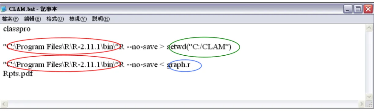
Right click the file “CLAM.bat”, and select “edit”. Then a Notepad window will appear as shown in Figure 1. Four modifications are necessary:

(1) Modify the source path for R (as indicated in Figure 1; red). For example, if your copy of R is installed in C:\Program Files\R\R-2.11.1\ (a default directory name when downloading R, where R-2.11.1 is the version of R), then modify the path to read: C:\Program Files\R\R-2.11.1\bin\. (Remember to add \bin\.) There are two instances of this path to be modified.

(2). Specify the source path (as indicated in Figure 1; green) for CLAM. For example, if the your CLAM directory is “C:\CLAM”, then it should be modified to

“setwd(“C:/CLAM”)”. (Please note the difference between forward slash and

backslash.)

(3). Specify the graph type (as indicated in Figure 1; blue). If you want a color graph, then keep the default, “graph.r”. If you prefer a black-and-white graph, then modify it to “graph(black-white).r”.

(3)

Remember to save and close this file after modifying it.

Figure 1. Setting up for CLAM by editing the text file CLAM.bat

Data Formats

All species frequency data must be stored in the tab-delimited plain text file called “data.txt”. When you download the program, data for the example used in Chazdon et al. (2011) are stored in “data.txt”. You must replace these with your own data in this file or replace the file with new file named “data.txt”. Data must be arranged in three columns, separated by tab characters: (1) species names, (2) frequency (or abundance) for Group A, and (3) frequency (or abundance) for Group B. An example in the

downloaded “data.txt” is shown in Figure 2. Space characters are not allowed in the column of species names. For example, the second species, Aegiphila falcata, should be modified to Aegiphila_falcata, Aegiphila.falcata or some other code for this species that contains no space characters. You can use Excel to edit the data first, and then save the file as “data.txt”, using the “Save AsTab-Delimited-Text” command from the Excel File menu.

(4)

Running Procedure and Output

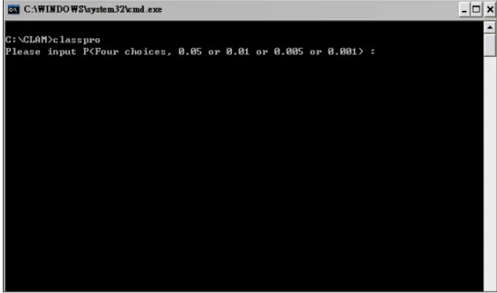
Step 1. After setting up the CLAM.bat file and the data input file, click the file “CLAM.bat” in the directory CLAM. Then the window for entry of

significance probability (P) in Figure 3 will appear. Input the value of P you require (there are four choices: 0.05, 0.01, 0.005 and 0.001). If your goal is to classify only one target species, P = 0.05 is suggested. If your target is to classify all species, P = 0.005 is suggested. (See Chazdon et al. 2011 for explanation of this recommendation.) After entry, click enter to save.

Figure 3. Interface window for P entry

Step 2. After Step 1, the interface window for entry of threshold K is shown as in Figure 4. The user should choose a threshold (K = 0.667 for super-majority threshold or K = 0.5 for simple-majority threshold). After entry, click enter to save. The program starts after the entry of K.

(5)

Figure 4. Interface window for K entry

When the program finishes computation, the CLAM.bat window will close, and there will be six new files in the directory CLAM: “List Table.xls,” “Count Table.xls,” “Rplots.pdf,” “pri_line.txt,” “sec_line.txt,” and “rare_line.txt.” The three files

“pri_line.txt,” “sec_line.txt,” and “rare_line.txt,” are just used for producing the graph, so these three files are not of any further use and can be ignored. The three useful output files are:

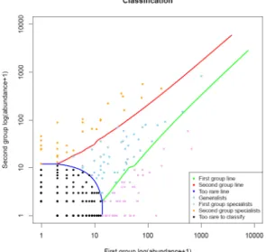
(1) “Rplots.pdf”: the classification plot of all species produced by R. An example is shown in Figure 5. In Program Settings, if you select “graph.r”, then a color plot will be obtained as in Figure 5a. If you select “graph(black-white).r”, then a black and white plot will be obtained as in Figure 5b.

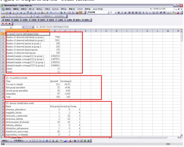
(2) “Count Table.xls” contains some basic information and the classification results. It contains three parts: Basic data information; Classificationsummary (number of species and percentages in each of the four categories: Generalist,First group specialist,Second group specialist and Too rare to classify); and Species

classification results (frequency data and classification category for each species), as shown in Figure 6.

(3) “List table.xls” contains species lists for each of the four classification categories (Generalist,First group specialist,Second group specialist and Too rare to classify). For each category, the species name, its abundance in the first group, and its

abundance in the second group are provided, as shown in Figure 7.

If you want to run any other data set, just repeat the above steps 1, 2, and 3 in the section “Running Procedure and Output.” However, before running additional

(6)

datasets, all six files must be closed, and the three useful files must be saved under different file names, because the six files will be replaced by the results obtained from running a new dataset. Each additional dataset must be in a file named “data.txt”.

Figure 5a. Classification Plot (color)

(7)

(8)

Figure 7. Output in the file “List table.xls”

Reference

Chazdon, R. L., Chao, A., Colwell, R. K., Lin, S.-Y., Norden, N., Letcher, S. G., Clark, D. B., Finegan, B. and Arroyo J. P. (2011). A novel statistical method for classifying habitat generalists and specialists. Ecology.