Program Life Cycle Cost Driver Model (LCCDM)
Daniel W. Miles, General Physics, June 2008
Introduction
Several years ago during the creation of the Periscope Total Ownership Cost (TOC) Program, it became very apparent that existing government processes and methods to assess TOC were not “user-friendly”. Documentation requirements were excessively detailed and difficult to use and, due to time constraints, most efforts were initially expended in interpreting these documentation requirements. Under these circumstances, it was very difficult to effectively provide a better understanding of the underlying program infrastructure costs and associated cost drivers that factor into the TOC process.
The development by General Physics Corporation (GP) of the P5 Cost Driver Model (CDM) subsequently provided a much needed TOC management tool to organize program cost data in a more efficient manner. The model distinguishes all program TOC factors as belonging to one of five possible basic cost driver categories — People, Paper, Parts, Performance, and Places. This classification approach provides for an easily understood graphical presentation of the five cost driver areas relative to TOC and enables a method to formulate and track the impact of specific cost drivers throughout program life-cycle activities for facilitating the development of cost reduction initiatives. With this insight, GP was able to interpret cost driver information that reduced program infrastructure and R&D costs and converted the savings into revenue flow for the program. The chart format in Figure 1 illustrates a typical generic example of profiling each of the five basic cost driver categories grouped together as a percentage of the total program expenditure. Several subcategories combine together to form each of these five main categories and will be broken down in more detail below.
Figure 1 – Generic Cost Driver Pie-Chart Profile
20%
20%
20% 20%
20%
People Paper Parts Performance Places
Phase Transitioning
Implementation of the Cost Driver Model on a cradle-to-grave government program usually involves segregating all identified costs into three logical life-cycle phases and constructing separate cost driver profiles typified by the following three chart figures. The first profile contains all Research, Development, Test, and Evaluation (RDT&E) costs which occur prior to the Acquisition (purchase) phase. This profile is typically dominated by non-recurring engineering design costs grouped within the Performance driver which directly affect the achievement of some operational requirement or performance specification. Figure 2 illustrates this point and also shows the relative representation of the impact to the total amount from the remaining cost drivers at this initial stage of sustainment.
Figure 2 – RDT&E Profile
The second profile contains all Acquisition costs required to purchase and install the system. Figure 3 illustrates percentages of costs from the model at this stage of the life-cycle sustainment. This profile now reflects the transition from a performance dominated phase to one exhibiting an increase in recurring costs such as Parts, system materials (fabricate or manufacture), and that of People required to build, install, and verify (test) system operation.
Figure 3 – Acquisition Profile
27%
9%
11% 51%
2%
People Paper Parts Performance Places
40%
19% 20%
17% 4%
People Paper Parts Performance Places
The third profile contains all Operation and Support costs necessary to maintain the system throughout its in-service life-span. Figure 4 illustrates the percentages of the cost drivers at this final stage of sustainment. The profile has now transitioned to one dominated by Parts costs. The maintenance actions of upgrades, technology refreshes, and repairs will exist until the entire system is replaced.
Figure 4 – Operation and Support Profile
In summary, all government programs follow an established sequence of transitional phases. Modeling of commercial programs appear to follow the same process, however different external forces affect the transition. Based on GP’s years of use with the Cost Driver Model, the following conclusions have been drawn:
• For any organization/project, People costs assume a range of 20% – 25% (with the exception of the Acquisition profile) for success. If the cost is below 18%, the organization/project slows down and becomes inefficient. If the costs are over 30%, the organization is either wasting or paying too much for resources.
• For any project, Paper costs are significantly less for commercial systems than that of government systems, by as much as a factor of 10.
• For any project, Parts costs increase through all profiles. In non-hardware projects, i.e. services, the Parts costs still reflect the dominant cost in the Operation & Support profile.
• For any project, Performance costs decrease through all profiles. Projects with a continuous improvement process, appear to maintain a constant level of performance, but are simply implementing new RDT&E profiles for each improvement. Eventually, in any performance improvement project/organization, the core requirement of the continuous improvement process will eventually be superseded by technology advancements.
• For any organization/project, Places costs are dependent on the profile requirements, but should not be more than 5% in any profile.
24%
10% 60%
6% 0%
People Paper Parts Performance Places
Applying Cost Driver Modeling for Life Cycle Sustainment
The life-cycle of a project starts in the RDT&E phase, followed by the Acquisition phase, and ends with the Operation and Support (O&S) phase. Following each phase, the Cost Driver Model allows for a feedback loop to any of the previous phases. This important feature enables smart management of variable program costs resulting in the ability to predict optimal allocation of resources for maximizing downstream savings. Table 1 provides a rough estimate of phase costs as a percentage of TOC as well as the amount to possibly save with intelligent cost budgeting.
Table 1 – Approximate Savings to TOC According to Program Phases
PHASE PERCENTAGE (%)
OF TOC
PERCENTAGE (%) OF POTENTIAL SAVINGS
RDT&E 10 20
Acquisition 20 10
Operation and Support 70 40
Cost Driver Subcategory Breakdown
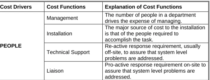
For each cost driver category there are associated cost functions. Table 2 illustrates an example of a government program where the cost functions for each of the five basic categories are explained. A similar table for commercial organizations/projects has been developed by GP.
Table 2 – Breakdown of Cost Driver Subcategories
Cost Drivers Cost Functions Explanation of Cost Functions
Management The number of people in a department drives the expense of managing. Installation
The major source of cost to the installation is that of the people required to
accomplish the task. Technical Support
Re-active response requirement, usually off-site, to assure that system level problems are addressed.
PEOPLE
Liaison
Pro-active response requirement on-site to assure that system level problems are
Cost Drivers Cost Functions Explanation of Cost Functions
Hardware System level components or a purchase requirement.
Spares Spares to system level components or a purchase requirement.
Software Required to support the system level components.
PARTS
Repair/Overhaul The action required to bring components to an RFI condition.
Facilities Areas where workers reside.
Laboratories Areas where development is conducted or equipment is maintained.
PLACES
Warehouses/Inventory Storage Areas
Areas where parts are maintained.
Engineering
Activities required to design a fix to a problem report/resolve a
deficiency/provide a system enhancement. SUBSAFE Activities/materials required to meet
SUBSAFE requirements.
PERFORMANCE
Quality
Assurance test activities required to demonstrate and verify system level performance.
Acquisitions Activities required to procure system level materials.
ILS Activities required to support logistics requirements for system level materials. CM Activities required to support configuration
management of system level materials.
PAPER
User Feedback
Activities required to
identify/maintain/report system level problem reports.
276 226
143 186
264 302
98 51 51
96 136
241 300
200
100 150
50 0
50 100 150 200 250 300 350
Accumulated Cost
($ Millions) 171
250 206
BREAK-EVEN BLOCK DRIVER BLOCK
PERFORMANCE BLOCK
COST BLOCK and LINKS PROCESS
Support &
Operation System
Baseline
Costs Support &
Operation System
New
OOM =
Objectives of the Life Cycle Cost Driver Model
The primary goal of the LCCDM process is to reduce costs in all phases of a program. To meet this goal, the model provides a metrics-based decision-making process created from meaningful data. The model also allows for smart assessments in the RDT&E and Acquisition phases that will minimize O&S costs. The modeling process evaluates the impact of technical cost drivers on performance, cost, and schedule. It supplements Earned Value Management (EVM) and risk factor identification by assessing cost driver elements through a Links process. It also supports achievement of the goals to reduce/meet the true break-even point by evaluating the technical progress towards achieving that goal.
Analytical Features of the Life Cycle Cost Driver Model
Figure 5 provides a visual generic presentation of the LCCDM illustrating all features of the process. The five blocks and links process are described below.
Performance Block
The performance block identifies the relative performance between a current baseline system and a proposed new system. The block provides a means to identify all requirements and compare them to existing or other proposed alternatives. The block allows the developer to determine if all requirements are met.
Performance Requirements New
SONAR System
Reference Document
Baseline Cost-Risk Value
(100%)
New System Cost-Risk Value
(100%)
MF Passive Common Spec 100 110
MF Active Common Spec 100 100
Transmit Group Common Spec 100 80
Self Noise Common Spec 100 95
Color Key
Green – System meets or exceeds existing system performance
Red – System does not meet existing system performance and needs to be fixed
Blue – System does not meet the existing system performance, however the required change is not cost effective requiring extensive system changes or a complete redesign
Driver Block
The driver block identifies the cost drivers of the proposed new system including risk mitigation costs and accelerators. An accelerator is an implementation of a project initiative that initially increases the cost within a phase but results in significant savings for follow-on phases thereby reducing program TOC. Utilizing the LCCDM Links functionality, the driver block aligns the proposed system elements between all three life-cycle sustainment phases. Reference sources of the data are required to support the analysis.
Cost Driver Cost Identifier Link Element Sub-Element
Integrated Product
Team (IPT) Risk Mitigation 10 Risk IPT
Sensors: Hydrophones Projectors
Driver: Minimal 31 Reliability Robustness
Connector/mold
configuration Driver: Moderate 401 Reliability Survivability
Cost Block
The cost block provides the media to assign projected, anticipated, and actual costs of the existing system with that of the proposed system. The costs are summarized to determine the total cost of any phase. The example provided is for Operation & Support (O&S) Costs.
Cost Driver Baseline
Cost
New System
Cost Sub Drivers
People 24%
Management
Financial Data Center Projects
Program
Personnel Installation
Implementation ALTS Certifications Planning
Installation Manager
Technical Assistance System Testing
System Integration Liaison
Performance 6%
Parts 60% Paper 10% Places < 1%
Links Process
The Links functionality generates cost driver/risk mitigation relationships for all identified elements in the model. The Links process also identifies relationships between the three phases of life-cycle costing, derives anticipated Link cost-multipliers, and implements accelerators that may result in cost increases/decreases based on decisions made during prior phases. The multiplier indicates the magnitude of such a potential reduction in cost savings. As indicated in Table 1, each phase has a different savings potential that could be achieved by implementing an accelerator initiative.
Output Ownership Metric (OOM) Block
The OOM block provides an assessment of how the changes made in the RDT&E and Acquisition phases are expected to affect O&S phase costs. A value greater than 1.0 indicates that the proposed new system will increase O&S costs above the current baseline system.
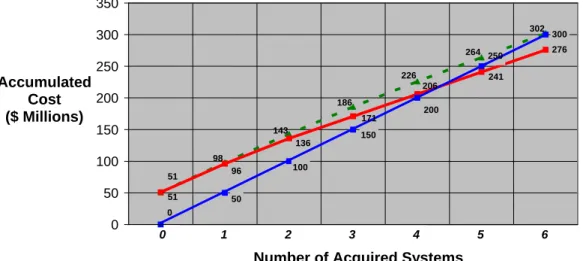
Break-Even/Learning Curve Analysis Block
The break-even/learning curve analysis block provides an accounting/earned value status as to the achievement in the Acquisition phase to recover the anticipated RDT&E project costs of a proposed new system. The graph in Figure 6 illustrates an example of break-even projection analysis for the GP cost driver model using realistic feedback that continuously fine-tunes cost driver relationships and updates model input data. This result is compared with a baseline projection (blue line) assuming a simple linear fixed-cost per system. An alternate analysis (red line) is also superimposed on the graph to show its projected breakeven point against the constant-sloped baseline. Although the alternate approach appears somewhat realistic by incorporating variable cost factors that reflect learning curve assumptions, it can actually lead to large errors in total cost expectations as the number of acquired systems increases. That is because of false (overly optimistic in
Support &
Operation System
Baseline
Costs Support &
Operation System
New = Metric Ownership
this case) input assumptions for values and relationships that multiply over time and generate significant offsets to the true break-even point.
Figure 6 – Break-Even/Learning Curve Projection Analysis for a Proposed RDT&E Project vs. a Current Baseline Acquisition System
276 226
143
186
264
302
98 51 51
96
136
241
300
200
100
150
50 0
0 50 100 150 200 250 300 350
Number of Acquired Systems Accumulated
Cost ($ Millions)
Cost Driver Model 51* 98 143 186 226 264 302
Alternate Analysis 51* 96 136 171 206 241 276
Baseline System 0 50 100 150 200 250 300
1 2 3 4 5 6
171
250
206
0
Total Acquisition Phase Cost Data ($M) as a function of Systems Acquired
Systems Acquired 0 1 2 3 4 5 6