Synchronization, Pliability and Resiliency
Christian Weiß
Submitted in accordance with the requirements
for the degree of Doctor of Philosophy
The University of Leeds
School of Computing
part of a jointly authored publication has been included. The contribution of the candidate and the other authors to this work has been explicitly indicated below. The candidate confirms that appropriate credit has been given within the thesis where reference has been made to the work of others.
Some parts of the work presented in Chapters 4, 5 and 6 have been published in the following articles:
C. Weiß, S. Waldherr, S. Knust, N. V. Shakhlevich (2016) Open shop scheduling with syn-chronization. Journal of Scheduling (published online), doi: 10.1007/s10951-016-0490-0, C. Weiß, S. Knust, N. V. Shakhlevich, S. Waldherr (2016) The assignment problem with
nearly Monge arrays and incompatible partner indices. Discrete Applied Mathematics 211, 183–203.
For both papers, all four authors worked on text, formulation, proof reading and literature search. In the first paper, scientific results (other than in Section 4) are mostly due to C. Weiß, though the other authors had large part in finding good presentation methods for this work. Results in Section 4 are due to S. Waldherr, N. Shakhlevich and C. Weiß.
In the second paper, results in Sections 2 and 3 are mostly due to C. Weiß. The result in Section 3 was achieved in collaboration with N. Shakhlevich. The first complete proof for the result in Section 4 was achieved by S. Waldherr and C. Weiß in collaboration. N. Shakhlevich played a large role in finding a good presentation for that work.
This copy has been supplied on the understanding that it is copyright material and that no quotation from the thesis maybe published without proper acknowledgement.
I would like to thank my supervisor Natasha Shakhlevich for her invaluable and patient support, starting from the application process and continuing through to the submission of this thesis. Without her help and guidance I would never have applied to study for a PhD in Leeds, let alone completed it. My thanks also go to my second supervisor, Martin Dyer, for providing helpful advice ever since joining my supervisory team.
Particular gratitude is also extended to Vladimir Deineko and Haiko M¨uller for examining this thesis and making many helpful suggestions for its improvement.
I am further grateful to our main collaborators Sigrid Knust and Stefan Waldherr for the time they invested in our joint work and for their hospitality when I visited them in Osnabr¨uck. Thanks for work put into our collaboration is also extended to Evgeny Gurevsky.
On a more personal (but at least equally important) note I want to thank all friends and colleagues who supported me both in Leeds and at home in Troisdorf: Sam Wilson and Thilo Simon for providing sounding boards for my ideas, especially in the early stages of my studies; Bj¨orn Buhr, Sebastian Kremer, Sebastian Heer and Sven Gießelbach for steadfast support and friendship since long before I started studying in Leeds; Emma Dobson, Ben White and others for providing friendship and company during my stay in Leeds; the people working in my office, especially Qingxu Dou and Fouzhan Hosseini; the PGR community both in the school and beyond, especially Marwan Al-Tawil, Alicja Piotrkowicz, Bernhard Primas and the alumni Matt Benathan and Elaine Duffin. Further thanks goes to the other members of my research group, those undergraduate students I had the pleasure of teaching during my time in Leeds, and many others, who I cannot name now, but who provided an invaluable social component and helped my find some balance during these busy three years.
Finally, I would like to give my deepest thanks to my parents, who have supported me and believed in me for much longer than any of the people named before even knew me.
In this thesis we study three new extensions of scheduling models with both practical and theoretical relevance, namely synchronization, pliability and resiliency. Synchronization has previously been studied for flow shop scheduling and we now apply the concept to open shop models for the first time. Here, as opposed to the traditional models, operations that are processed together all have to be started at the same time. Operations that are completed are not removed from the machines until the longest operation in their group is finished.
Pliability is a new approach to model flexibility in flow shops and open shops. In schedul-ing with pliability, parts of the processschedul-ing load of the jobs can be re-distributed between the machines in order to achieve better schedules. This is applicable, for example, if the machines represent cross-trained workers.
Resiliency is a new measure for the quality of a given solution if the input data are uncertain. A resilient solution remains better than some given bound, even if the original input data are changed. The more we can perturb the input data without the solution losing too much quality, the more resilient the solution is.
We also consider the assignment problem, as it is the traditional combinatorial optimization problem underlying many scheduling problems. Particularly, we study a version of the assign-ment problem with a special cost structure derived from the synchronous open shop model and obtain new structural and complexity results. Furthermore we study resiliency for the assignment problem.
The main focus of this thesis is the study of structural properties, algorithm development and complexity. For synchronous open shop we show that for a fixed number of machines the makespan can be minimized in polynomial time. All other traditional scheduling objectives are at least as hard to optimize as in the traditional open shop model.
Starting out research in pliability we focus on the most general case of the model as well as two relevant special cases. We deliver a fairly complete complexity study for all three versions of the model.
Finally, for resiliency, we investigate two different questions: ‘how to compute the resiliency of a given solution?’ and ‘how to find a most resilient solution?’. We focus on the assignment problem and single machine scheduling to minimize the total sum of completion times and present a number of positive results for both questions. The main goal is to make a case that the concept deserves further study.
Contents
1 Introduction 1
2 Preliminaries 5
2.1 Necessary notation from graph theory . . . 5
2.2 General definitions and notation for scheduling . . . 7
2.2.1 A general scheduling problem . . . 7
2.2.2 The three-field notation . . . 8
2.3 Scheduling models . . . 11
2.3.1 Single machine scheduling problems . . . 11
2.3.2 Scheduling problems with parallel identical machines . . . 13
2.3.3 Scheduling problems with parallel uniform machines . . . 14
2.3.4 Flow shop problems . . . 14
2.3.5 Open shop problems . . . 15
2.3.6 Job shop problems . . . 16
2.4 The linear assignment problem . . . 16
2.4.1 The two-dimensional linear assignment problem . . . 17
2.4.2 Matching problems in bipartite and general graphs . . . 18
2.4.3 The multi-dimensional linear assignment problem . . . 19
2.4.4 The linear assignment problem with Monge costs . . . 19
I
Synchronization
23
3 Definitions, notation and related work 25 3.1 Introduction and definitions . . . 253.2 Related work . . . 27
4 Synchronous Open Shop Scheduling with Two Machines 31 4.1 Minimizing the makespan . . . 31
4.1.1 ProblemO2|synmv|Cmax . . . 32
4.1.2 ProblemO2|synmv, rel|Cmax . . . 44
4.2 Scheduling with deadlines . . . 49
4.3 Minimizing the total completion time . . . 54
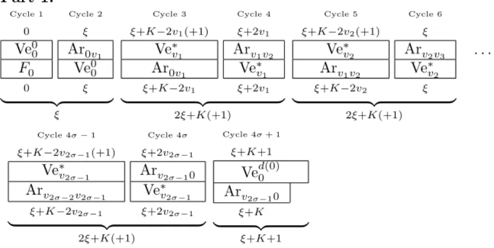
4.4 Details for the NP-hardness ofO2|synmv|PC j . . . 62
5 The Assignment Problem with Nearly Monge Arrays and Incompatible Part-ner Indices 77 5.1 Introduction . . . 77
5.2 Applications . . . 80
5.3 NP-hardness of problem AP(d, λ) . . . 83
5.4 Some properties of nearly Monge matrices with incompatible partner indices . . 87
5.4.1 Nonexistence of a Monge sequence . . . 87
5.4.2 Recognizing nearly Monge arrays . . . 88
5.4.3 Completing nearly Monge arrays . . . 90
5.5 The corridor property for problem AP(d, λ) . . . 91
5.6 A linear-time algorithm for problem AP(d, λ) with fixeddandλ . . . 97
5.7 The corridor property for other versions of the assignment problem . . . 101
5.7.1 Axial three-dimensional assignment problem with decomposable costs . . 101
5.7.2 Planar 3-dimensional assignment problem with a layered Monge matrix . 103 5.7.3 Bottleneck assignment problem with a bottleneck nearly Monge matrix and its generalizations . . . 106
5.8 NP-completeness of 3-DM with incompatible partner indices . . . 107
6 The relaxed problem O|synmv, rel|Cmax 111 7 Conclusions and further research 115 7.1 Synchronous open shop scheduling . . . 115
7.2 Assignment problem with a nearly Monge matrix . . . 116
7.3 Further research for synchronous scheduling models . . . 120
II
Pliability
123
8 Definitions, notation and related work 125 8.1 Introduction and definitions . . . 1258.2 Related work . . . 127
9 Shop scheduling problems with pliable jobs 131 9.1 General properties and reductions . . . 131
9.1.1 Pliability of type (i) . . . 131
9.1.2 Pliability of type (ii) . . . 133
9.2 Type (i) problems with minmax criteria . . . 138
9.2.1 Type (i) problemsF|plbl|Cmax andO|plbl|Cmax . . . 138
9.2.2 Type (i) problemsF|plbl|Lmaxand O|plbl|Lmax . . . 139
9.3 Type (ii) problems with minmax criteria . . . 141
9.3.1 Type (ii) problemF|plbl(p)|Cmax . . . 141
9.3.2 Type (ii) problemO|plbl(p)|Cmax . . . 144
9.3.3 Type (ii) problemF|plbl(p)|Lmax . . . 146
9.4 Type (iii) problems with the makespan objective andm= 2 . . . 148
9.4.1 ProblemF2|plbl(pij, pij)|Cmax . . . 148
9.4.2 ProblemO2|plbl(pij, pij)|Cmax . . . 150
9.5 Type (i) and type (ii) problems with min-sum criteria . . . 153
9.5.1 Type (i) problemsF|plbl|P Cj andO|plbl|PCj . . . 153
9.5.2 Type (ii) problemF|plbl(p)|PC j . . . 155
9.5.3 Type (ii) problemO|plbl(p)|P Cj . . . 156
9.5.4 Other problems with min-sum criteria . . . 159
9.6 Proof of Lemma 36 . . . 163
10 Conclusions and further research 169 10.1 General observations . . . 170
10.2 Pliability of type (i) and (ii) withn < m . . . 171
10.3 Further research . . . 173
III
Resiliency
175
11 Definitions, notation and related work 177 11.1 Introduction . . . 17711.2 Related work . . . 181
11.2.1 Stability . . . 182
11.2.2 Robustness . . . 184
12 Resiliency for Combinatorial Optimization Problems with Uncertain Data 187 12.1 General Properties . . . 187
12.1.1 Complexity Aspects . . . 188
12.1.2 Properties of objective functions that limit the search for worst-case de-viations . . . 188
12.1.3 Problems with the`∞-norm . . . 190
12.2 The Assignment Problem with Uncertain Costs . . . 191
12.2.1 The assignment problem with arbitrary fluctuation factors . . . 191
12.2.2 Assignment problem with binary fluctuation factorsαij ∈ {0,1} . . . 200
12.3 Problem 1||PC
j with uncertain cost . . . 208
12.3.1 The case with arbitrary fluctuation factorsαj for the job processing times 209 12.3.2 The case with binary fluctuation factorsαj∈ {0,1} . . . 215
12.3.3 ProblemP||P Cj . . . 218
13 Conclusions and Further research 221 13.1 Advantages and challenges of the resiliency concept . . . 221
13.2 Generalization and transfer of our results to other problems . . . 223
13.2.1 Resiliency for 0−1 combinatorial optimization problems . . . 223
13.2.2 Resiliency for list scheduling problems . . . 224
13.2.3 Resiliency for other scheduling problems . . . 225
13.3 Future research – a broader view . . . 226
13.3.1 Interval based resiliency . . . 226
13.3.2 Resiliency for linear programming . . . 227
List of Figures
2.1 Reductions between traditional scheduling objectives . . . 10
4.1 Gantt chart of an optimal schedule for Example 2 . . . 34
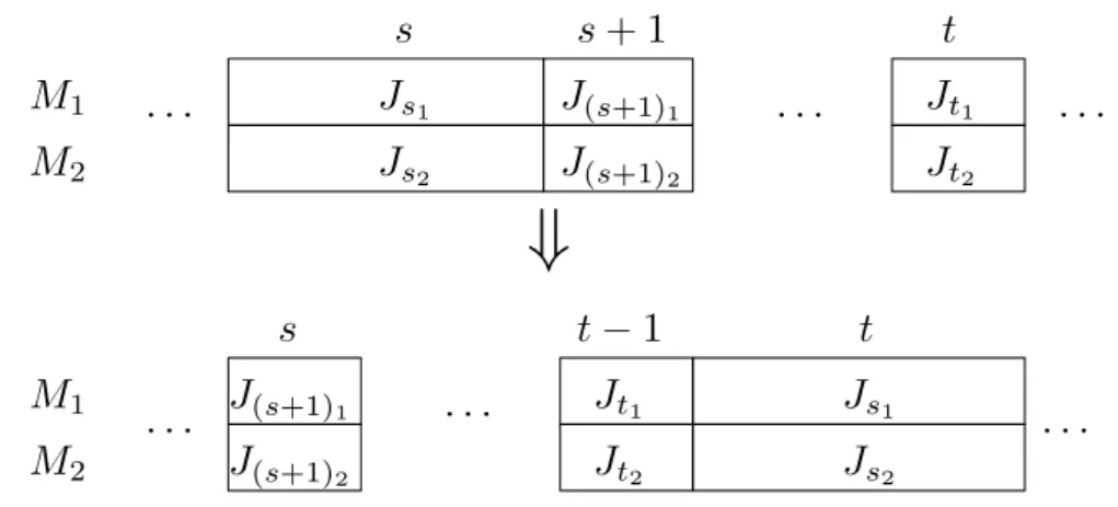
4.2 Transformation of blockXy intoX0y . . . 37
4.3 Transformation of blockXy into ¯Xy . . . 37
4.4 Cases wheret= 2 and a=u≤3: (a)a=u= 1, (b)a=u= 2, (c)a=u= 3 . . 38
4.5 Transformation fromXy toXey . . . 38
4.6 Transformation fromXey toXeey . . . 39
4.7 Transformation fromXy toXby . . . 40
4.8 Transformation fromXby toXbby . . . 40
4.9 Transformation fromXy toX∗y . . . 41
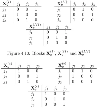
4.10 BlocksX(yI),Xy(II)andX(yIII) . . . 42
4.11 BlocksX(ya),Xy(b)and X(yc) . . . 42
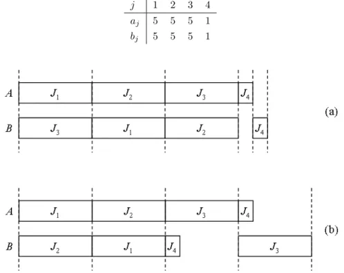
4.12 Two open shop schedules, Cr max < Cmax∗ : (a) An optimal schedule with one dummy job paired with job 1; (b) An optimal schedule without dummy jobs. . . . 45
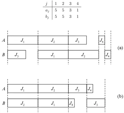
4.13 An example illustrating that conditions (4.11) are not sufficient for introducing a dummy job: (a) an optimal schedule with one dummy job; (b) an optimal schedule without dummy jobs. . . 49
4.14 Schedule derived from a solution to 3-PART . . . 51
4.15 Constructing the graph −→G for problem AUX . . . 55
4.16 An optimal solution to SO . . . 58
4.17 Structure of schedule S . . . 60
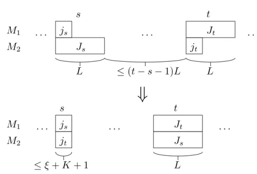
4.18 Creating a cycle of long operations and a cycle of short operations ifJs6=Jtand js6=jt . . . 65
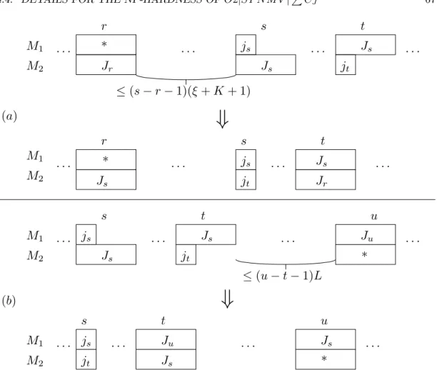
4.19 Creating a cycle of long operations and a cycle of short operations if Js = Jt, js6=jt and (a) there is a long operation in cycler, r < s, (b) there is no long operation in any cycler,r < s, but there is a long operation in cycleu,u > s . . . 67
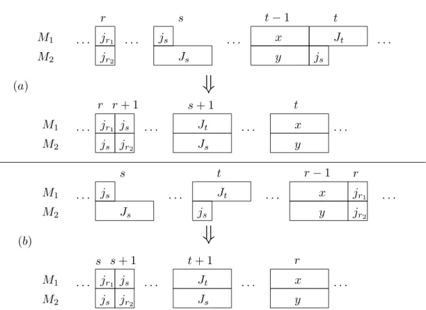
4.20 Creating a cycle of long operations and a cycle of short operations if Js 6=Jt,
js=jtand there is a cyclerwith two short operations,
(a)r < s,
(b)r > s. . . 68
4.21 Moving long cyclesafter a sequence of short cyclesU ={s+ 1, . . . , t} . . . 70
4.22 A special short cycle appearing among the last 2(n9+ 1) cycles . . . 70
5.1 A feasible transmission schedule for Example 19 . . . 82
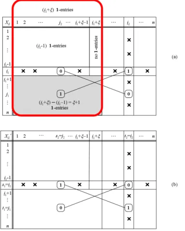
5.2 Eliminating Type I(i2) violation (a) Solution matrixXS with the violatingd-tuple (i1, i2, . . . , id) of Type I(i2) (b) Modified solution matrixX0 S with Type I(i2) violation in rowi1 eliminated . 93 5.3 Eliminating Type II(i2) violation (a) Solution matrixXS with the violatingd-tuple (i1, i2, . . . , id) of Type II(i2) (b) Modified solution matrixX0 S with Type II(i2) violation in rowi1 eliminated . 95 6.1 An optimal schedule forO3|synmv|Cmaxand an improved schedule forO3|synmv, rel|Cmax (with dummy jobJ6) . . . 112
6.2 An optimal schedule with 2mcycles,mof which are complete andmare incomplete113 9.1 Adjacent jobs swap: (a) schedule S; (b) scheduleS0 . . . 134
9.2 SchedulesSe ∗ andS∗d for instancesIeandId, and the combined scheduleS∗ optimal for instanceI . . . 136
9.3 The disjunctive graph representation of scheduleSd . . . 137
9.4 Modifying an optimal schedule forP|pmtn|Cmax intoF-type andO-type sched-ules by adding zero-length operations . . . 139
9.5 An optimal solution to an instance ofF|plbl|Lmax with Ω(mn) non-zero operations140 9.6 A schedule for the instance with processing times given by (9.10) in which – job 1 is split such that it has processing time 3.5 on each machine and – job 1 is scheduled continuously between in [0,10.5] . . . 145
9.7 An optimal solution to the instance of the flow shop problem . . . 149
9.8 A schedule for problemF|plbl|P Cj in staircase form . . . 153
9.9 Two equivalent schedules optimal for (a)P|pmtn|P CjandP||PCj(b)F|plbl|PCj154 9.10 The start of a schedule for problemO|plbl(p)|PC j . . . 158
9.11 Adding the second Latin square of operations . . . 158
9.12 A complete schedule for problemO|plbl(p)|P Cj with 8 jobs . . . 159
9.13 Pre-processing: - introducing intervals [`0 i, ri0]⊆[`i, ri] for each machineMi, 1≤i≤m; - decomposing schedule S into two subschedules with machines {M1, M2, M3} and{M4, M5}under the condition`04+p≥r30 . . . 164
11.1 The B-feasible region and resiliency balls for an instance of problem 1||PC
j
List of Tables
4.1 Processing times of the jobs in instance SO . . . 56 7.1 Summary of the results for synchronous open shop scheduling . . . 115 7.2 The summary of complexity results for problemAP(d, λ) . . . 117 10.1 Open shop and flow shop problems with pliable jobs and minmax objectives . . . 169 10.2 Open shop and flow shop problems with pliable jobs and minsum objectives . . . 170 12.1 Examples of scheduling problems that can be modelled as assignment problems . 192 12.2 Upper bounds of the search space for different examples of combinatorial
opti-mization problems . . . 199
Introduction
The area of scheduling has received continuous interest from researchers for more than sixty years. Originating from industrial production and machine scheduling, today scheduling re-search has many different applications in public and commercial service provision. A famous description of the area as a whole is due to Pinedo [121], who stated that “Scheduling deals with the allocation of scarce resources to tasks over time. It is a decision making process with the goal of optimizing one or more objectives.”
Over the years many standard models and their extensions have been studied, leading to different types of results, including exact algorithms, complexity theorems, approximation algorithms, heuristics and mathematical programming formulations. However, new interesting questions still emerge frequently. As industry is faced with new challenges, more and more often managers turn to operational research to help optimize the processes in their companies. Either the models derived from such a request may be completely new, or they may be similar to one of the well-known classical models with one or more additional, unstudied features.
In this thesis, we consider problems of the latter type, where known models are enhanced by special features. These features can arise, for example, from government regulations (e.g. health and safety), special set ups of industrial plants, measures taken by a company to im-prove work flow (e.g. cross-training) or measures for solution quality (e.g. energy efficiency or fairness). We investigate three of these features more closely, namely synchronization, pliability and resiliency. Our interest lies in complexity study, exact polynomial time algorithms and underlying structural results to help guide heuristic approaches in the future.
Synchronization has previously been studied for flow shop scheduling, where jobs have to be processed by a sequence of specialized machines, one after the other, in order to obtain the finished products. This is a standard setting, for example, in industrial plants. In a traditional flow shop scheduling problem machines are numbered, and each job has to be processed by the machines in order of their numbering, starting with the first machine, then the second and so on. For synchronous flow shop we additionally require that the jobs are moved from one
machine to the next one all at the same time. The main applications for synchronous flow shop models come from industrial plants with special job movement provisions. Consider a set up where machines are connected via the same transportation unit (e.g. a common conveyor belt). In that case, when the transportation unit moves forward, it moves all jobs at the same time.
We consider the extension of synchronous scheduling to open shop. Here, as for flow shop, a production process consists of several steps for each product, each step executed by a specialized machine. The difference between the traditional open shop and flow shop scheduling models is that the requirement to be processed by the machines in order of their numbering is lifted for open shop. Instead, for each job it is part of the decision process in which order it is processed by the machines. Again, for the model with synchronization job changes on the machines have to be made at the same time. Applications for synchronous open shop arise for example from health and safety regulations. If workers need to change jobs on the machines manually, then all machines may have to be stopped for workers to be able to safely enter the machine room. Unless job changes are at the same time, this procedure causes a large overhead in the production process.
The second feature, pliability, is interesting for shop scheduling environments, and we again focus on flow shop and open shop problems. The main assumption is that workers are cross-trained, and can take over some work from other workers. This helps reduce overheads that appear when solving regular shop scheduling problems. It has been noted by several authors ([37, 38, 39]) that this kind of “flexibility” can greatly improve the overall efficiency of a produc-tion environment. While several related models have been studied in the literature, pliability is a completely new feature, and we initiate research in this area by considering the most general version of pliability, as well as a couple of interesting special cases.
Lastly, resiliency is a new measure for solution quality in cases where the problem data are uncertain. Traditionally, when solving scheduling problems, it is assumed that processing times as well as other problem parameters are exactly known beforehand. In reality, often the problem parameters are not available as exact data, but rather as estimates. Furthermore, practitioners are frequently not in need of strictly optimal solutions, and are instead satisfied with solutions that are good enough, i.e. they do not exceed a certain threshold or are better than what they had before. These two observations motivate the search for resilient schedules, which are defined by the following two conditions. First, they should not exceed a given threshold of the objective function for the given parameter estimates. Second, they should not lose too much quality and continue to lie within the threshold, even if the actual problem parameters differ slightly from the original estimates.
As with pliability, resiliency has not previously been considered in literature. It is related to the well-known concepts of robustness [4] and stability [140]. Our contribution is to provide the necessary definitions to start the research in this area and to provide some initial general results, as well as an example of deeper study into a couple of specific problems and identification of promising further research questions.
A secondary area of interest in this thesis is the linear assignment problem, which plays a role in several chapters as an underlying model, both in its general version and in versions with special cost matrices. The linear assignment problem is well-studied in the literature [25]. In the two dimensional version we have to find an assignment of elements of one set to elements of another set, i.e. finding pairs. The goal is to minimize the cost of the assignment, which can be computed as the sum of the costs of each individual pair. The costs of the pairs are usually given in form of a cost matrix W = (wij), where entry wij denotes the cost of assigning the
i-th element of set one to the j-th element of set two. A standard example of an application from scheduling is assigning tasks to workers, where the cost of a task-worker pair is the time it takes for the worker to complete the assigned task. If the tasks have to be completed one after the other, then the total time it takes to finish the product is equal to the sum of times that each worker needs for their task.
For the higher dimensional version, with d dimensions, we are givend sets and instead of finding pairs we have to findd-tuples, which include exactly one element from each of the sets. For example, when assigning final year projects in the academic sector, we need to consider projects, supervisors and students. The cost for a project-supervisor-student triple is guided by the preference of the student for the project and the expertise of the supervisor in the project area.
The complexity status of the linear assignment problem, both for two and more dimensions, has been known for many years. In general, it is solvable in O(n3) time [84, 88] for d = 2
dimensions and strongly NP-hard for all higher dimensionsd≥3 [80, 84]. However, things are different if the cost matrices associated with the assignment problem have special structures.
A famous example is the so-called Monge condition. Anm×nmatrixW = (wij) is called
a Monge matrix, if for all 1≤i < r≤mand 1≤j < s≤nwe have wij+wrs≤wis+wrj.
Monge matrices give rise to very efficient algorithms for many types of optimization problems, such as the linear assignment problem, the (Hoffman) transportation problem and the travelling salesperson problem (see the survey paper [26]). In particular, for the linear assignment problem it can be shown that if the cost matrix is Monge, then the problem can be solved in linear time [26]. The same still holds for the multi-dimensional linear assignment problem, if the above Monge condition is generalized for multi-dimensional arrays.
Our contribution in this area is the definition of a new Monge-like cost structure, which has several applications. For this structure we study the assignment problem in particular, which is shown to arise from the synchronous open shop problem. We prove that assignment problems of this type are solvable in linear time as long as the dimension dis fixed, and not part of the input. We also study resiliency for the general version of the assignment problem.
This thesis is structured as follows. In the next chapter we provide notation, definitions from the areas of graph theory, scheduling and the assignment problem needed throughout
this thesis, as well as a few traditional results related to our later research. After that, the thesis is divided into three independent parts, one for each of the three features we study, synchronization, pliability and resiliency. In addition to the general introduction in the next chapter, each part also has its own introductory section, where additional notation and related work pertaining only to the contents of the respective part is discussed.
In Part I, the main focus is on scheduling synchronous open shops. We show that for any fixed number of machines minimizing the length of the schedule is polynomially solvable. Other traditional scheduling objectives are strongly NP-hard to solve even for two machines. We also discuss an underlying assignment problem and prove a new structural property for the solution of an assignment problem with a cost matrix of Monge-like structure.
Part II is about pliability. We define the model and provide an initial complexity study for the most common objective functions. Furthermore, we suggest several promising directions to extend the model for further research.
The new concept of solution resiliency is investigated in Part III. We define resiliency for the case of a general combinatorial optimization problem and compare this definition to related concepts in the literature. Then we provide some general results and study two specific prob-lems in greater depth: the two-dimensional linear assignment problem, as it underlies many scheduling problems, as well as scheduling on a single machine to minimize the total sum of completion times.
Preliminaries
In this chapter we provide an overview of definitions and notation which are used in the thesis as a whole. We also discuss related work and important results pertaining to some of the notions introduced.
Due to the nature of the work presented in this thesis, there are also definitions and notation only needed in specific chapters. These are not presented here, instead they are introduced in the appropriate places inside the chapters, in which they are used. Any related work is also presented at that time. Furthermore, to keep this section concise, we omit a general introduction to combinatorial optimization and complexity theory. For such introductions see [59] or more modern texts like [84]. An introduction to algorithms is also given in [33].
We start by introducing some elements of graph theory in Section 2.1. In Section 2.2 some general notions from scheduling theory are established, with a focus on those areas which are needed later in the thesis. The specific models closer related to our work and the classical results concerning those models are discussed in more detail in Section 2.3. The linear assignment problem, which is important in several places throughout the thesis, is introduced in Section 2.4. We repeat results both for the general cases and for the versions with Monge cost structures, which are explained as well.
2.1
Necessary notation from graph theory
This section is a concise introduction of the key concepts of graph theory needed for this thesis. The main goal is to provide the notation used for graphs in this thesis. For a more thorough and detailed introduction to graphs see, e.g., [44] or for a more algorithmic focused introduction the appropriate chapters in [84].
A graph G= (V, E) consists of avertex set V and anedge set E, where an edgee∈E is a two-elemental subset ofV. Ife={v, w} ∈E for two verticesv, w∈V thenv andware called
adjacent and eis called incident with v and w. The degree degG(v) of a vertex v ∈ V is the
number of edges incident withv. We may also write deg(v) if there can be no confusion about the graph in question.
Atrailorwalk of lengthkin graphGis a sequence of vertices (v0, v1, v2, . . . , vk), such that
{vi, vi+1} ∈E for alli= 0,1,2. . . , k−1. Ifv0=vk then the trail is calledclosed or acircuit.
A trail is called a path ifvi and vj are different for each choice of 0≤ i < j ≤k other than
{i, j} = {0, k}. A path is called a cycle if v0 = vk, i.e. if it is closed. A graph G is called
connected if for each pair of vertices v, w∈Gthere exists a path (of some length) inGwhich starts inv and ends inw. A graphGis calledacyclic if it does not contain a cycle.
A graphG= (V, E) is called complete if{v, w} ∈E for allv, w∈V, v6=w. The complete graph withnvertices is unique up to isomorphisms and is denoted byKn. A graphG= (V, E)
is calledbipartiteif the vertex setV can be partitioned into two subsetsV1andV2, such that for
each edge{v, w} ∈Ewe havev∈V1andw∈V2. A complete bipartite graphG= (V1∪V2, E)
is a bipartite graph such that {v, w} ∈E for all v ∈V1 and w∈ V2. The complete bipartite
graph withmvertices in one vertex set andnvertices in the other is unique up to isomorphisms and is denoted by Km,n.
Given a graph G = (V, E) then its line graph L(G) is defined as the graph which has as vertex set the edge set ofG, and two edges ofGare adjacent vertices inL(G) if they are incident with the same vertex inG, i.e.L(G) = (E, L(E)), whereL(E) ={{e1, e2} ⊂E:|e1∩e2|= 1}.
Adirected graph ordigraphG= (V, E) is defined similarly, only that the edges additionally have a direction. In this case edges are given as ordered pairs e = (v, w) ∈ E such that E ⊆ V ×V. If e = (v, w) ∈ E then e is called an outgoing edge of v and an incoming edge of w. The in-degree deg−G(v) of a vertex v in an undirected graph G is the number of
edges in G entering v. The out-degree deg+G(v) is the number of edges leaving G. Again,
the degree degG(v) is the number of edges incident with v, both entering and leaving, i.e.
degG(v) = deg
+
G(v) + deg−G(v).
Adirected trail or directed walk of lengthk in a directed graphGis a sequence of vertices (v0, v1, v2, . . . , vk) such that (vi, vi+1) ∈ E for all i = 0,1,2, . . . , k−1. Directed paths and
directed cycles defined analogously. A directed graph Gis strongly connected if for each pair of vertices v, w ∈ G it contains a directed path of some length that starts in v and ends in w. It isweakly connected if the underlying undirected graph obtained fromGby dropping the directions on all edges is connected. A directed graphGis calledacyclic if it does not contain a directed cycle.
Given a directed or undirected graph G = (V, E) a trail in G is called a (directed or undirected)Eulerian trail or Eulerian walk if it uses every edge inGexactly once (it may use vertices multiple times). An Eulerian trail is called Eulerian tour or Eulerian circuit if it is closed. A undirected graphGisEulerianif every vertex inGhas even degree. A directed graph G is called Eulerian if for every vertexv in G we have deg−G(v) = deg+G(v). It is well-known that a (strongly) connected directed or undirected graphGis Eulerian if and only if it contains an Eulerian tour (see, e.g., [84]).
A directed or undirected path/cycle in a directed or undirected graph G is called Hamil-tonian path/cycle if it includes every vertex inG. A directed or undirected graphG is called
Hamiltonian if it contains a Hamiltonian cycle.
2.2
General definitions and notation for scheduling
In this section we introduce basic definitions and notation from scheduling theory. We start by presenting a very general notion of a scheduling problem and a feasible schedule. After that, we introduce the three-field notation, the normal manner in which scheduling problems are denoted.
2.2.1
A general scheduling problem
For a general scheduling problem a set of njobsJ ={J1, J2, . . . Jn} needs to be processed on
a set m machines M ={M1, M2, . . . , Mm}. Throughout the thesis, if there is no ambiguity,
we use a simplified notation J ={1,2, . . . , n} for jobs andM={A, B} if there are only two machines.
Each job j, 1≤j ≤n, consists ofnj ≥1 operations{O1j, O2j, . . . , Onjj}. OperationOιj,
1≤ι≤nj, is associated with a processing timepιj and a subsetµιj ⊂ Mof machines by which
it may be processed. Then the operationOιj has to be processed on one of the machines inµιj
forpιj time units.
Nearly everywhere in this thesis it is enough to consider one of two special cases for the number of operations per job nj and the setsµιj. In the first case each job j has only one
operation O1j, i.e. nj = 1 for all jobs j and µ1j = M. We identify job j with its single
operation and denote its processing time by pj. Examples for scheduling models of this type
are introduced in Sections 2.3.1–2.3.3. In the second case each job has m operations, one operationOij for each machineMi, withµij={Mi}, i.e. operationOij has to be processed by
machineMi. In both cases, in order to reduce notation, we drop the indexιfor the operations.
Examples for scheduling models of this type are introduced in Sections 2.3.4 and 2.3.5. The only scheduling model used in this thesis that does not belong to one of these two cases is job shop scheduling, which is introduced in Section 2.3.6.
A schedule S is an allocation of each operation Oιj to a machine Mi ∈ µιj and a time
interval Iιj = [Tιj, Tιj+pιj) on machineMi. We call Cιj =Tιj +pιj the completion time of
operationOιj andCj = max{Cιj|ι= 1, . . . , nj}the completion time of jobj. For a schedule to
be feasible we usually require that no job is processed by two machines at the same time and no machine processes two jobs at the same time:
F1 the time intervalsI1j, I2j, . . . , Injjbelonging to the operations of jobjare pairwise disjoint,
Additional requirements for feasibility can arise depending on the model at hand. For example, in addition to the above, a schedule may have to respect release dates or deadlines associated with the jobs. If job j has a release date rj, then no operation of job j may be
processed before time rj. Similar, if job j has a deadline Dj, then all operations of job j
have to be processed by time Dj. If release dates and deadlines are given, the following two
requirements for a feasible schedule are added:
F3 for each jobj and each operationOιj we haverj≤Tιj,
F4 for each jobj we haveCj ≤Dj.
Note that instead of deadlines, jobs can also have due dates, denoted bydj for each jobj. The
difference is that feasible schedules may violate due dates (for a cost), soF4is not added for due dates. Due dates are of importance for several scheduling objectives, which will be explained in greater detail later on.
Also, the set of operations belonging to a job j, may be partially ordered by precedence constraints. This is the case if some operations belonging to jobj need to be completed before other operations belonging to the same job j can be started. The precedence constraints are usually given in the form of an acyclic directed graphG, whereOι1jhas to be processed before
Oι2j if there is a path inGfrom the vertex associated withOι1j to the vertex associated with
Oι2j. Formally, the following additional requirement needs to be satisfied by a feasible schedule:
F5 if operationOι1j is required to be processed before operationOι2j, thenCι1j≤Tι2j.
For this thesis, it is enough to consider precedence constraints which are represented by a directed path O1j →O2j →O3j →. . . →Onjj, as happens for flow shop scheduling and job
shop scheduling (see Sections 2.3.4 and 2.3.6.
It is possible for some requirements to be newly introduced or relaxed if the investigated model calls for this. For example, for a feasible schedule in models with synchronization it is required that operations which are processed in intersecting time intervals are started at the same time (see also Chapter 3). On the other hand, requirementF2is relaxed for multiprocessor or batching machines, which can compute several operations simultaneously. See [17] for details and other examples.
2.2.2
The three-field notation
Scheduling models are classified using the so-called three-field notation,α|β|γ, whereαspecifies the machine configuration, β specifies job characteristics and special processing requirements and γ specifies the optimization goal. The notation was first introduced in [65]. A general introduction to the three-field notation is provided in [17].
Machine configurations
The machine configurations are explained in greater detail in Section 2.3. The four most important machine configurations for this thesis are parallel identical machines, parallel uniform machines, flow shop and open shop. They are denoted by α=P, α=Q, α=F andα=O respectively. Additionally, there may be a number after the letter, to specify the exact number of machines, e.g. α=F2 for two-machine flow shop. If no number is given, then we assume the number of machines is part of the input. If there is only one single machine, then this is denoted byα= 1.
Job characteristics
Theβ-field specifies any non-standard characteristic of the jobs or processing requirements. We provide a few important examples here and introduce other entries when they are used.
– If release dates or deadlines are given, then this is specified by the entryrj orDj
respec-tively in the β-field.
– If all jobs have the same processing time, then this is specified by the entry pj =pin the
β-field. For unit processing times we writepj = 1. Similar specifications may happen for
release dates, deadlines or due dates.
– If pmtn appears in the β-field, then operations may be interrupted at any time during their processing and later restarted on the same machine, or on another machine that can process them. This may happen several times for the same operation, leading to several intervals in which the operation is processed, rather than only one. However the full processing time of the operations must still be scheduled before the operation is completed. All other requirements for a feasible schedule apply as well.
– The entry p−batch in the β-field indicates that parallel batching is allowed on the machines. Parallel batching is introduced in Section 2.3.1.
Optimization goals and objective functions
Finally, the optimization goal in theγ-field usually is a combination of one or more objective functions, though for this thesis only optimization goals consisting of a single scheduling objec-tive are considered. In general, a scheduling objecobjec-tive is given by a functionf(C1, C2, . . . , Cn)
dependent on the completion timesC1, C2, . . . , Cnof the jobs. The goal is then to find a feasible
schedule which minimizes the objective functionf. The most important scheduling objectives for this thesis are the following:
– the makespanCmax= max{C1, C2, . . . , Cn}, i.e. the completion time of the last completed
– the sum of completion timesPC
j =Pnj=1Cj;
– the maximum latenessLmax= max1≤j≤n(Cj−dj) for given due datesdj.
Other prominent scheduling objectives are the total tardiness PT
j =Pnj=1Tj with Tj =
max{0, Cj−dj}and the number of late jobsPUj =Pnj=1Uj, with
Uj=
(
1 ifCj > dj,
0 otherwise.
For each of the min-sum objectives there also exists a weighted version, with weightswjgiven for
each job, i.e. the weighted sum of completion timesPw
jCj =Pnj=1wjCj, the weighted total
tardiness P
wjTj=Pnj=1wjTj and the weighted number of late jobsPwjUj=Pnj=1wjUj.
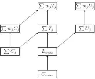
Elementary reductions are well known for these traditional scheduling objectives, see, e.g., [17]. For example, by setting all weights wj = 1 we can see that the unweighted min-sum
objectives are special cases of the weighted ones. Therefore, the weighted versions are at least as hard to minimize as their respective unweighted versions. Similarly, if all due dates are equal, then minimizing the maximum lateness reduces to minimizing the makespan. Conse-quently, the makespan objective is a special case of the maximum lateness objective and the maximum lateness is at least as hard to minimize as the makespan. The elementary reductions for traditional scheduling objectives are presented in Fig. 2.1, see, e.g. [17].
Figure 2.1: Reductions between traditional scheduling objectives
Note that all of the objectives mentioned here are non-decreasing in the completion times. An objective function f(C1, C2, . . . , Cn) which is non-decreasing in the completion times is
called regular. In this thesis we normally deal with regular objective functions. Objectives which are not regular arise, for example, in just-in-time scheduling, see, e.g., [9]. An example of such
an objective is the combined total earliness and total tardiness,P(E
j+Tj) =Pnj=1(Ej+Tj),
whereEj = min{0, Cj−dj}.
2.3
Scheduling models
Since this thesis is about scheduling models with additional features it is natural to start with a summary of the traditional models from which they are derived. We focus on complexity results and exact polynomial time algorithms for the most important and general problems (with the least additional requirements and assumptions in the β-field). If more specialized results are needed in places later in the thesis, they are provided there.
For a broader or more detailed introduction to scheduling models we recommend [17] or [121]. A useful overview of complexity results in form of tables is also given on the web page [19], though the tables are also partially available in [17].
2.3.1
Single machine scheduling problems
For scheduling problems with only one machine we usually assume that each job consists of only one operation. Recall that in this case, we identify with the job itself and the processing time of a job j is denoted by pj. Below we first summarize briefly the results for classical
single machine scheduling which are interesting for this thesis, then we move on to scheduling a batching machine, as it is an important related model for the later part on synchronization.
Classical single machine scheduling
Problem 1||Cmax is trivial, as each schedule without idle times is optimal. Problem 1||Lmax is
solvable in O(nlogn) time by scheduling jobs, without idle times, in order of non-decreasing due dates [17, 77]. This is called Jackson’s rule or simply EDD-rule (earliest due date first).
Minimizing the total completion time 1||P
Cj is also done O(nlogn) time by scheduling
jobs, without idle times, in order of non-decreasing processing times [17, 139]. This is known as Smith’s rule or SPT-rule (shortest processing time first). As a generalization, problem 1||P
wjCj is solvable inO(nlogn) time by scheduling jobs in order of non-decreasing ratio wpjj.
This is known as Smith’s ratio rule [17, 139]. Finally, problem 1||PU
j is solved O(nlogn) time by Moore’s algorithm [17, 115]. First
schedule jobs in order of non-decreasing due dates. Then, if the job in positionjis the first late job in the sequence, move the job with the largest processing time amongst all jobs in positions 1,2,3, . . . , j to the end of the sequence. The process is repeated, again with the position of the first late job in the sequence. It is stopped when all jobs are either on time or have been moved to the end of the schedule during the algorithm. The resulting optimal schedule is in two parts, all on-time jobs in the beginning of the schedule, in order of their due dates, and all late jobs are at the end of the schedule in any order.
For the other traditional scheduling objectives f ∈ {PT
j,PwjTj,PwjUj} problem 1||f
is NP-hard. To be more precise, problems 1||P
Tj and 1||PwjUj are NP-hard in the ordinary
sense (see [49, 91] and [80, 99] respectively), while problem 1||Pw
jTj is strongly NP-hard
[91, 102].
For this thesis the above summary suffices in terms of introduction to classical single machine problems. A more detailed collection of results, which includes additional job characteristics like release dates or precedence constraints, can be found in [17].
Scheduling a batching machine
There are two types of batching models: serial batching (s-batching) and parallel batching (p-batching). In this thesis only the latter model is of interest. For an introduction to s-batching see [17].
If parallel batching is allowed on a machine, then part of the decision process is to partition the job set into batches. All jobs of a batch are processed in parallel and the processing time of a batch is equal to the processing time of the longest job within the batch. The completion time of a job is equal to the completion time of the batch to which the job belongs. Instead of sequencing jobs, as we did for the classical problems above, we first partition jobs into batches and then sequence the batches on the machine.
There are two variants dependent on the maximum batch-size b, the number of jobs any batch may contain. In unrestricted p-batching we have b ≥ n, i.e. a batch may contain ar-bitrarily many jobs. In that case the maximum batch size is not denoted in the three-field notation and the problem is denoted by 1|p−batch|f, iff is the objective function. In re-stricted p-batching we have b < nand no batch may contain all jobs. The problem is denoted by 1|p−batch, b < n|f if the maximum batch size is part of the input or 1|p−batch, b= ¯b|f if the maximum batch size is fixed to some integer ¯b. Note that in general even in the restricted model it is not required that batches are filled up to the maximum batch size and batches may contain fewer thanbjobs.
In general, unrestricted p-batching is much easier than restricted p-batching. Indeed, for unrestricted p-batching only problems 1|p−batch|P
wjUj and 1|p−batch|PwjTj are proven
to be NP-hard (in the ordinary sense) with 1|p−batch|PT
j still open. All other traditional
scheduling objectives f ∈ {Cmax, Lmax,PCj,PwjCj,PUj} can be optimized in polynomial
time; see [17] and [18] for details.
Conversely, the only polynomial algorithm known for restricted p-batching (without any additional special assumptions) is for problem 1|p−batch, b < n|Cmax [17, 18]. Here jobs are
assigned to a batch in order of non-increasing processing times until the maximum batch size is reached, then a new batch is started with the next job. The problem is solvable inO(nlogn) time, due to sorting.
All problems involving due dates are strongly NP-hard to solve even for maximum batch size b= 2, i.e. 1|p−batch, b= 2|f is strongly NP-hard forf ∈ {Lmax,PTj,PUj,PwjTj,PwjUj}
[18].
Problems 1|p−batch, b < n|PC
j and 1|p−batch, b < n|PwjCj are open, to the best of
our knowledge.
2.3.2
Scheduling problems with parallel identical machines
In this section we discuss scheduling parallel identical machines. As for single machine schedul-ing, each job has only one operation. Any job can be processed by any of the machines and all machines take the same amount of time pj to process a given job j. We first summarize
results for scheduling identical parallel machines without preemption, after that we turn to the preemptive case.
Parallel identical machines without preemption
Note that any NP-hardness result from single machine scheduling carries over to scheduling parallel machines. Therefore problemP2||Pw
jTj is strongly hard, due to the strong
NP-hardness of the single machine problem with the same objective.
Furthermore, even for two machines, minimizing the makespan is equivalent to the PAR-TITION problem. Indeed, the minimum makespan of Ppj
2 can be achieved if and only if the
set of processing times can be partitioned into two sets with the same sum of elements. Thus, problem P2||Cmax is NP-hard in the ordinary sense [102]. ProblemP||Cmax with the number
of machinesmpart of the input is strongly NP-hard to solve [58]. The situation is similar for the objective functions f ∈ {Lmax,PTj,PUj,PwjUj} instead of f =Cmax. See [17] for a
detailed set of references.
Using an extension of Smith’s rule we can solve problem P||P
Cj in O(nlogn) time, by
sorting jobs in order of non-decreasing processing times and then repeatedly assigning the shortest unassigned job to the first free space on any machine.
Finally, problemP2||Pw
jCjis NP-hard in the ordinary sense [21] and problemP||PwjCj
is strongly NP-hard [17].
Parallel identical machines with preemption
For the preemptive case, McNaughton showed that problemP|pmtn|Cmax is solvable in O(n)
time [111]. First the optimal makespan is computed, then machineM1is filled with jobs until
the optimal makespan is reached. At that point, the current job is preempted and restarted on the next machineM2. The remaining schedule is built in a similar manner.
Problem P|pmtn|Lmax is solvable in O(nlogn) time by Sahni’s algorithm [133] combined
with an algorithm to compute the optimal maximum lateness for a given instance [11].
Minimizing the number of late jobs for a fixed numbermof machines, i.e. problemP m|pmtn|PU
j,
is solvable inO(n3(m−1)) time [92, 93, 98], whileP
||P
Uj with the number of machinesmpart
in the ordinary sense even for two machines, because the single machine problem with objective functionP
wjUj is NP-hard, both with and without preemption.
It is a well known result that for problem P|pmtn|P
wjCj an optimal schedule without
preemption exists [111]. Consequently, problem P|pmtn|PC
j is solvable in O(nlogn) time
(by the same method as in the non-preemptive case) whileP2|pmtn|P
wjCjis NP-hard in the
ordinary sense, again by [21]. Finally, problemsP2|pmtn|PT
j andP2|pmtn|PwjTj are NP-hard in the ordinary sense
and in the strong sense respectively, due to the NP-hardness results for problems 1||P Tj and
1||Pw
jTj. Note that for the preemptive versions of the single machine problems there exist
optimal schedules without preemptions.
2.3.3
Scheduling problems with parallel uniform machines
Now we turn our attention to scheduling problems with parallel uniform machines. Again, each job has only one operation and may be scheduled on any machine. The difference to the model with identical machines is that now machines may have different processing speeds. If the processing time of jobjispj then the actual time it takes for machineMiwith speedsi to
process job j is pj
si.
Note that problems with parallel identical machines can be seen as special cases of the problems with parallel uniform machines where all machine speeds are equal to 1. Thus, all NP-hardness results known for parallel identical machines carry over to parallel uniform machines.
While the exact running times of algorithms may differ, the complexity status (i.e. NP-hard or polynomially solvable) of the problems Q||f and Q|pmtn|f with uniform machines and a traditional scheduling objective f, is the same as that of the related problems with identical machines. Indeed, problem Q||PC
j is solvable in polynomial time while
optimiz-ing any other traditional scheduloptimiz-ing objective is at least NP-hard in the ordinary sense, even for two machines. Similarly, problems Q|pmtn|f with f ∈ {Cmax, Lmax,PCj} are
polyno-mially solvable (see [89] for the latter two objectives), while the problems Q2|pmtn|f with f ∈ {P
wjCj,PTj,PwjTj,PwjUj} are at least ordinarily NP-hard. Finally, again like for
parallel identical machines problemQm|pmtn|PU
jis solvable in polynomial time, while
prob-lem Q|pmtn|P
Uj is NP-hard.
For this thesis we leave our introduction at that. More details and references beyond the ones already given in Section 2.3.2 can be found in [17].
2.3.4
Flow shop problems
In flow shop scheduling we consider problems with m machines and n jobs, where each job has exactly moperations and for all jobsj operationOij has to be processed by machineMi.
have to be completed, i.e. the set of operations of each job is ordered by precedence constrains given by the graph O1j → O2j → O3j → . . . →Omj. For scheduling objectives which make
the introduction of voluntary idle times (idle times which are not forced by the constraints of a feasible schedule) unnecessary, such as the makespan objective, the problem is to find for each machineMi the sequence in which the jobs are processed on machineMi.
The most well-known classical result for flow shop scheduling is that problem F2||Cmax is
solvable in O(nlogn) time by Johnson’s algorithm [79]. First we partition the job set J into two subsetsJ1={j ∈ J |p1j ≤p2j}andJ2={j ∈ J |p1j > p2j}. Then we construct the first
part of the schedule by sequencing on both machines all jobs in setJ1in order of non-decreasing
processing time p1j. Once all jobs in setJ1 are sequenced, in the second part of the schedule
we sequence on both machines all jobs in setJ2in order of non-increasing processing timep2j.
A schedule in which the sequence of jobs is the same on each machine, like the one con-structed by Johnson’s algorithm is called a permutation schedule. Johnson’s algorithm proves that an optimal permutation schedule exists for problemF2||Cmax. Optimal permutation
sched-ules also exist for problemF3||Cmax (see, e.g., [17]). For four or more machines, this property
no longer holds. Counterexamples for the case with four machines are provided, for example, in [122].
In terms of complexity, Johnson’s result remains the only positive one unless additional assumptions are made. Indeed, problems F3||Cmax, F2||Lmax andF2||PCj are all strongly
NP-hard ([60] and [102]). Consequently problemF2||f is also strongly NP-hard for each tradi-tional scheduling objectivef other than the makespan.
Even allowing preemption does not improve the situation. Indeed, problem F2|pmtn|Cmax
is again solvable in O(nlogn) time [63], while problems F3|pmtn|Cmax, F2|pmtn|Lmax and
F2|pmtn|PC
j are strongly NP-hard, like their non-preemptive counterparts ([63] for the
makespan, [31] for the maximum lateness and [50] for the total sum of completion times). For now we leave it at this general introduction as it is not practical to introduce more specialized results at this time. However, flow shop plays an important role in this thesis and more results are discussed in the parts of the thesis where those results are needed.
2.3.5
Open shop problems
Open shop is similar to flow shop, in that each job has exactlymoperations and for all jobsj operationOij has to be processed by machineMi. However, the precedence constraints between
operations of one job are dropped, making it part of the decision process which operation of a job is processed first, second and so on.
In general, open shop scheduling is usually slightly easier than flow shop scheduling. The famous result by Gonzalez and Sahni [62] shows that problemO2||Cmax can be solved in linear
time. In the algorithm, the two jobs with the largest operations on the two machines are treated separately, while the order of all other jobs only depends on whether p1j ≤p2j or p1j > p2j.
ProblemsO3||Cmax andO|n= 3|Cmax are NP-hard in the ordinary sense [62]. Minimizing
the makespan becomes strongly NP-hard for problemO||Cmax, i.e. if the number of machines
m is part of the input [17]. All other traditional objectives are strongly NP-hard to minimize even for two machines, as for flow shop (see [95, 96] for the maximum lateness and [1] for the total sum of completion times).
With preemption allowed, open shop again appears to be slightly easier than flow shop. Problems O|pmtn|Cmax and O|pmtn|Lmax, with the number of machinesm arbitrary, can be
solved in polynomial time by linear programming [31]. The result still holds, even if release dates are given in addition. For problem O|pmtn|Cmax there also exists an algorithm which
finds an optimal solution inO(rmin{r, m2
}+mlogn) time, whereris the number of operations with non-zero processing time, i.e. r ≤ nm [62]. Problem O2|pmtn|P
Cj is NP-hard in the
ordinary sense [50], while problem O3|pmtn|P
Cj is strongly NP-hard [105]. Finally problem
O2|pmtn|PU
j is NP-hard in the ordinary sense [95, 96].
This is where we stop our general introduction. Extensions to open shop scheduling are a key part of this thesis and in the subsequent parts we turn our attention to more specialized results that are directly related to our work.
2.3.6
Job shop problems
We conclude our review of classical scheduling models with a brief introduction to job shop scheduling. Job shop, denoted byJ in theα-field of the three-field notation, is a generalization of flow shop, where a job j can have arbitrarily many operations nj and for each operation
Oιj there is some dedicated machineMi on which it must be processed, in which case we have
µιj ={Mi}. Still, as in flow shop, operationOι∗j cannot be started before all operationsOιj,
ι < ι∗, are completed. Flow shop is a special case of job shop wherenj =mfor all jobs j and
µij ={Mi}, for all 1≤i≤m and 1≤j≤n.
The job shop model does not play a large role in this thesis. We do not provide a summary of results as we did for the previous models and we only introduce it here as it is convenient to do so immediately after introducing the other two shop scheduling problems. Clearly all NP-hardness results from flow shop carry over. Below we give two additional results, one negative and the other positive, as examples. For a more thorough summary see [17].
First, as an additional NP-hardness result, problem J2||Cmax is strongly NP-hard even if
there are only two different processing times pιj ∈ {1,2} for all operations Oιj [101]. As a
positive result, problemJ2|nj≤2|Cmax, where each job as at most two operations, is solvable
in O(nlogn) time [78].
2.4
The linear assignment problem
As the last part of this chapter we introduce the linear assignment problem, focusing on the balanced case, wherenobjects in one set need to be assigned tonobjects in another set. The
unbalanced case, wheremobjects in the first set need to be assigned tonobjects in the second, m < n, and some of thenobjects are not assigned is not relevant for this thesis. We also discuss the closely related matching problems in bipartite and in general graphs. First we introduce the two-dimensional linear assignment problem in Section 2.4.1 and the matching problems in bipartite and general graphs in Section 2.4.2. Then we turn to multi-dimensional assignment problems in Section 2.4.3. Finally, in Section 2.4.4, we introduce the Monge condition and explain how the complexity of the linear assignment problem changes when Monge costs are involved.
2.4.1
The two-dimensional linear assignment problem
The assignment problem is an important combinatorial optimization problem with many ap-plications in different areas (see, e.g., [25]). In this problem the objective is to assignn items of one set I ={1, . . . , n} to n items of another set J = {1, . . . , n}, where I may represent a set of workers, jobs, transmitting devices, andJ may correspond to machines, rooms, receivers, etc. In the linear assignment problem, additionally ann×nweight (cost) matrixW = (wij) is
given, and the goal is to find an assignment with minimum total weight.
An assignment S may be represented by a set of n pairs, S ={(i1, j1), . . . ,(in, jn)
} with
{i1, i2, . . . , in
}={j1, j2, . . . , jn
}={1,2, . . . , n} and it is characterized by the weight
w(S) = X
(i,j)∈S
wij.
An assignmentS is also called asolution and a solution S∗ with minimum weight is called an
optimal solution.
An alternative representation of the assignment problem uses binary decision variables xij
indicating the assignment of i-items toj-items: min n P i=1 n P j=1 wijxij s.t. n P j=1 xij = 1, 1≤i≤n, n P i=1 xij = 1, 1≤j≤n, xij ∈ {0,1}, 1≤i, j≤n. (2.1)
Clearly, there exists a one-to-one correspondence between any solutionSand the binary solution matrixXS = (xij) withxikjk = 1 for every pair (ik, jk)∈S, 1≤k≤n. The linear assignment
problem can be solved in polynomial time, e.g., by the Hungarian algorithm [88], which can be implemented to run inO(n3) time [25].
We can also represent a solution to the assignment problem as a permutation
The solution S given by the pairsS={(i1, j1), . . . ,(in, jn)
} is represented by permutationπS
with πS(ik) = jk, such that S = {(i1, πS(i1)),(i2, πS(i2)), . . . ,(in, πS(in))}. Furthermore, in
that case the solution matrixXS as defined above is the permutation matrix corresponding to
permutationπS in the usual definition of permutation matrices (see, e.g., [20], p. 2).
2.4.2
Matching problems in bipartite and general graphs
The linear assignment problem is closely related to weighted matching problems in graphs. Given a graphG= (V, E) amatching M inGis a subset of the edges,M ⊆E, such that in the graph G(M) = (V, M) no vertex has degree larger than 1. A matchingM∗ is calledmaximal, if adding any edge e∈E\M∗ to M∗ would destroy the matching property, i.e. would cause
one vertex in G(M∗) to have degree two. A matchingM∗ in Gis amaximum matching ofG, if|M∗|= max{|M|:M is a matching inG}. Finally, a matching M∗ in Gis calledperfect, if
every vertex inGis matched byM∗, i.e. inG(M∗) every vertex has exactly degree 1. Observe that in that case we have |M∗|= |V|
2 .
If in addition the edges ofGare weighted by a weight functionw:E→R, then the weight
of a matchingM inGis defined by
w(M) = X
e∈M
w(e).
Given a graphG= (V, E), the minimum weight perfect matching problem is to find a perfect matching of minimum weight inG[84], or to decide that no perfect matching exists.
Matching theory is a vast field on its own, see [107] for a detailed introduction. We focus on the relation of the minimum weight perfect matching problem to the assignment problem and provide two general complexity results needed in this thesis.
If G = (V1 ∪V2, E) is a bipartite weighted graph with V1 = {v1, v2, . . . , vn} and V2 =
{vn+1, vn+2, . . . , v2n}, then the minimum weight perfect matching problem inGcan be
trans-formed into an assignment problem with weight matrix W = (wij) given by
wij =
(
w({vi, vn+j}), ife={vi, vn+j} ∈E,
∞, otherwise.
Clearly, if a perfect matching exists in G then the solution to the assignment problem with weight matrix W can be transformed into a perfect matching in G with minimum weight. Conversely, if no perfect matching exists inG, then any solution to the assignment problem has infinite weight. Therefore, ifGis a bipartite graph, then the minimum weight perfect matching problem can be solved inO(n3) time with the same methods as the assignment problem (see
also [84]).
IfGis a general graph, not necessarily bipartite, then the structure of a solution becomes much harder to grasp. According to [84], minimum weight perfect matching in general graphs is
one of the “hardest” polynomially solvable combinatorial optimization problems. We do not go into detail here and simply cite the result that the problem is still solvable inO(n3) time by a
weighted version of Edmond’s blossom algorithm. The algorithm was first proposed by Edmonds [51], then Gabow [55] and Lawler [90] independently found the first O(n3) implementations. The currently best theoretical time bound ofO(nm+n2logn) was again obtained by Gabow
[56]. See also [84] for details. Practical implementation of the algorithm is still an issue today, see [83].
2.4.3
The multi-dimensional linear assignment problem
The extension of the linear assignment to the multi-dimensional case gives rise to the so called
axiald-dimensional assignment problem (d≥2): given ad-dimensionaln× · · · ×nweight array W = (wi1...id), an assignmentS is a set ofn d-tuples{ i
1 1, . . . , i1d , i2 1, . . . , i2d , . . . ,(in 1, . . . , ind)} with{i1
`, . . . , in`}={1, . . . , n} for all`= 1, . . . , d, and its weight is
w(S) = X
(i1,...,id)∈S
wi1...id.
The formulation in terms of the binary decision variablesxi1...id is as follows:
min P i1,...,id wi1...idxi1...id s.t. P i1,...,id s.t. i`=k xi1...id= 1, 1≤`≤d, 1≤k≤n, xi1i2...id ∈ {0,1}, 1≤i1, i2, . . . , id≤n. (2.2)
The associated solution array XS = (xi1...id) has a 1-entry xi1...id = 1 for every d-tuple
(i1, . . . , id) = ik1, . . . , ikd
∈ S, where 1 ≤ k ≤ n. Note that in any solution XS, the
num-ber of 1-entries isn, while the remainingnd
−nentries are 0.
Unlike the two-dimensional version, the d-dimensional assignment problem is strongly NP-hard for each fixedd≥3, see, e.g., [80].
In relation to matchings, the problem can be interpreted as finding minimum weight per-fect matchings in hypergraphs (e.g. 3-dimensional matching, see [59]), which is strongly NP-complete.
2.4.4
The linear assignment problem with Monge costs
There exists a multitude of special cases, which have been of interest to researchers and for which the assignment problem can be solved faster than in cubic time (see, e.g., [25]). In what follows, we introduce one of these special cases that is of major interest for us, namely assignment problems with Monge costs. The Monge property indicates a special structure of the cost matrix, and has a long history of study going back to Gaspard Monge in 1781 [114].
It is well known that many combinatorial optimization problems, including the assignment problem, can be solved faster (by a greedy algorithm) if the weight matrix is a Monge matrix. We remind here the main definitions and results following the survey paper [26]. An n×n matrixW = (wij) is called aMonge matrix if for all row indices 1≤i < r≤nand all column
indices 1≤j < s≤nthe so-called Monge property is satisfied:
wij+wrs≤wis+wrj. (2.3)
An optimal solution to the assignment problem with a Monge matrix is given by the n pairs (1,1),(2,2), . . . ,(n, n). Thus the assignment problem is solvable inO(n) time, if the cost matrix is Monge.
A number of typical applied scenarios with Monge and Monge-like arrays are discussed in the survey papers [24] and [26]. As an example from scheduling, problem 1||P
Cj famously
can be formulated as an assignment problem with Monge cost (see also [26]). Given a sequence of jobs (j1, j2, . . . , jn) as a solution to problem 1||PCj, note that the total completion time
for the corresponding schedule is X
Cj = Cj1+Cj2+Cj3+. . .+Cjn−1+Cjn
= pj1+ (pj1+pj2) + (pj1+pj2+pj3) +. . .+ (pj1+pj2+pj3+. . .+pjn−1)
+(pj1+pj2+pj3+. . .+pjn−1+pjn)
= npj1+ (n−1)pj2+ (n−2)pj3+. . .+ 2pjn−1+pjn.
The jobjkin positionkcontributes its own processing timepjkto the objectiven−k+ 1 times.
We can model problem 1||P
Cj as assigning jobs to positions in the sequence. If a solution
S to the assignment problem is given, then in the corresponding solution sequence for the scheduling problem job j is in position i if (i, j) ∈ S. The cost matrix W = (wij) for the
assignment problem is given by
wij = (n−i+ 1)pj.
If the jobsjare numbered in non-decreasing order of processing times, then for indices 1≤i < r≤nand 1≤j < s≤nwe have
wij+wrs= (n−i+ 1)pj+ (n−r+ 1)ps≤(n−i+ 1)ps+ (n−r+ 1)pj=wis+wrj
and the matrix W is Monge.
The Monge property can be generalized to multi-dimensional arrays. Ann× · · · ×narray W = (wi1...id) is called a (d-dimensional) Monge array if for alli`, j`∈ {1, . . . , n},`= 1, . . . , d,
we have
ws1s2...sd+wt1t2...td≤wi1i2...id+wj1j2...jd, (2.4)
multi-dimensional assignment problem with a Monge array is given by then d-tuples (1, . . . ,1), (2, . . . ,2),. . ., (n, . . . , n). Again, the problem is solvable inO(n) time.
Note that in many texts on Monge structures (e.g. [26, 124]), results for the assignment problem are presented in their generalized form for the closely related transportation problem. In its usual, continuous form, thed-dimensional transportation problem is formulated as follows:
min P i1,...,id wi1...idxi1...id s.t. P i1,...,id s.t. i`=k xi1...id=a ` k, 1≤`≤d, 1≤k≤n, xi1i2...id ≥0, 1≤i1, i2, . . . , id≤n. Here a`
k are given non-negative suppl