Stability and Shapes of Cellular Profiles in Directional Solidification: Expansion and Matching Methods

244 Journal of Crystal Growth 112 (1991)244—282 North-Holland

Review paper

Stability and shapes of cellular profiles in directional solidification:

expansion and matching methods

John D. WEEKS

*,

Wim van Saarloos

** A T& TBell Laboratories, Murray Hill, New Jersey 07974, USA

and

Martin Grant

Department of Physics, McGill University, Montreal, Quebec, Canada H3A 2T8

Received 15 October 1990

Ideas based on constitutional supercooling suggest that the periodic steady state cellular patterns seen in the directional solidification of systems with small partition coefficient may beunstableif the impurity concentration in the melt just in front of the tips falls into the two phase (miscibility gap) region of the phase diagram. This gives a simple stability criterion relating the position of the tips of the cells to the pulling velocity that is in good qualitative agreement with the limited experimental data available in the cellular regime. Implications of this criterion for a particular class of steady state solutions derived using asymptotic matching methods are explored. These solutions arise from a generalization to finite Péclet number for systems with small partition coefficient of the ideas of Dombre and Hakim relating directional solidification patterns to viscous (Saffman—Taylor) fingers. Families of steady state solutions yielding both small amplitude interface patterns as well as fingerlike solutions with narrow deep grooves are accurately described by the methods discussed herein. A systematic expansion method provides corrections to the classical Scheil shapes for the grooves. However, the stability criterion, as well as other considerations, suggest that the entire class of narrow grooved solutions found by the matching methods may be unstable. Comparison with other numerical work suggests that other branches of narrow grooved solutions exist and are relevant to experiments. Several experimental and numerical tests of these ideas are proposed.

I. Introduction

quite complex (and difficult to study

experimen-tally), at somewhat larger pulling speeds typically

A variety of interesting patterns can form dur-

one encounters finite amplitude steady state

pat-ing the directional solidification of a binary mix-

terns like that shown in fig. la, or fingerlike cells

ture [l—3]. In this technologically important pro-

with deep grooves as in fig. lb. These figures are

cess, solidification occurs when a thin sample of

taken from theoretical work by Ungar and Brown

melt is pulled through a fixed temperature gradi-

[4], but experimental examples of both kinds of

ent. As the pulling speed V is increased, the initial

patterns have been observed by Trivedi [5] in the

planar solid—liquid interface becomes unstable.

succinonitrile—acetone system and, more recently,

While the detailed behavior very near threshold is

by de Cheveigné and coworkers [6] in the CBr4—Br2

system. An example of cells with grooves observed

* Present address: Institute for Physical Science and Tech-

in experiments of Cladis et al. [7] is shown in

nology, University of Maryland, College Park, Maryland

f~ 2

20742,USA.

g.

.

* * Present address: Instituut Lorentz. University of Leiden,

A convenient way to display the experimental

Nieuwsteeg 18, 2311 SB Leiden, Netherlands.

results is to plot the wavelength A of cellular

J. D. Weeks et a!.

/

Stability and shapes ofcellular profiles in directional solidification 245

L

2 0

_{concentrated on a steady state analysis. Recent}

Most theoretical studies of these patterns have

MELT ,

work, both numerical and analytic, has established

1

that the steady state equations describing

direc-tional solidification (DS) admit a

continuous family

71

2.5

of periodic solutions of varying wavelengths for a

given set of experimental conditions. Dombre and

2 4

Hakim [10] carried out a particularly elegant

ana-lytic demonstration of this fact for a simplified

model of DS with a partition coefficient of unity

2 52

3.0

in the limit that the Péclet number p tended

towards zero. (The Péclet number p compares the

2 94

scale of the pattern to the range of the diffusion

SOLID

CRYSTAL

3.5

(0)

(b)

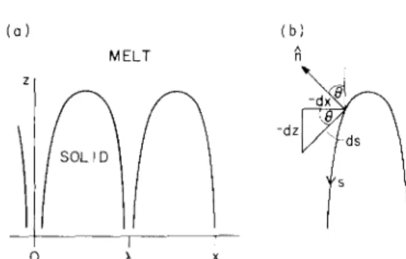
Fig. 1. Examples of the cell profiles calculated numerically by Ungar and Brown

14,731.

The thin solid lines show the iso-con-centration lines. (a) A finite amplitude cell at Péclet number

p= XV/2D 0.4, v =1.2, a 0.026. (b) Half of a cell with a I

groove at Péclet numberp=XV/2D =0.4, p 1.33 and a =

0.016. The parameter a is defined in eq. (9.1).

patterns versus the pulling velocity

V,

and

com-pare this scale to the length scales associated with

a linear stability analysis of the planar interface.

Such a plot is reproduced in fig. 3 from the work

I

of de Cheveigne et al. [8]. In this figure, the

I

wavelength of perturbations about the planar

in-terface that are neutrally stable (i.e. neither grow

I

nor decay) is indicated by a solid line. (Note that

•

the neutrally stable modes represent valid steady

state solutions of infinitesimal amplitude). Curves

for two different temperature gradients are shown.

The minimum threshold velocity

V~

at which the

planar interface first goes unstable is denoted by

the square symbol at the bottom of the curves.

I

Perturbations about the planar interface with

wavelengths in the wide band between these two

solid lines are linearly unstable; we therefore refer

to this region as the planar instability band. The

Fig. 2. Example of some experimental cell patterns at three

selected cells for a given pulling velocity in the

different moments in time, showing the periodic release of

experiments of de Cheveigné et al. [8] have wave-

bubbles fromthe bottom ofa groove.The initialprofileisthe

lengths that lie within the planar instability band

one on thebottom, and thesepictures were taken while the cellular region was expanding into the planar region on the

in the narrow dashed region whose wavelength is a

. .

246 J. D. Weeks et al.

/

Stability and shapes of cellular profiles in directional solidification

band for which a family (or families’) exists

I0~

according to a simple steady state analysis.

Very near threshold, one typically expects [14]

I

that the band of stable periodic nonlinear

solu-102 -

tions lies within the planar instability band (near a

supercritical (forward) bifurcation, this follows

I

from the Eckhaus instability results for the

ampli-tude equations [15]). Unfortunately, however, for

10 -

directional solidification, the amplitude

expan-sions [16] and bifurcation analysis [17] on which

(b)

these conclusions are based are valid only

ex-tremely close to threshold, when

(V— V

)/

V.<<

1.

4 ~ . . C C

1 10 102 io~

This is because the bottom of the neutral stability

WAVELENGTH (pm)

curve illustrated in fig. 3 is extremely flat in most

Fig. 3. Plot of the growth velocity versus wavelength for the

cases, so expansion methods quickly break down

experiments of de Cheveigne et al. [8]. The solid line marks the as the velocity is increased. (The important excep-neutral stability wavelength as a function of the growth veloc-

tion [18] is the regime where the partition

coeffi-ity for two values of the thermal gradient G.Expenments for . .

(a) G=120°C/cm(•)and (b) G=70°C/cm(0) lie in the cient k is close to 1, as is the case for liquid narrow shaded band. The dashed line indicates the minimum

crystals [19].) However,

recent results

by Brattkus

deep cell wavelength calculated in this paper, and the arrows

and Misbah [20] on the stability boundary of

illustrate that the matched asymptotic expansion employed in

strongly nonlinear solutions confirm that for their

this paper is an expansion towards larger wavelength. See text.

particular model the band of stable nonlinear

solutions lies within, but is significantly narrower

field in front of the pattern. See section 2 for

than, the planar instability band. The mechanism

precise definitions.) In this limit a formal analogy

that governs the wavelength selection within the

with the equations describing viscous fingering in

stable band they find still remains an unsolved

a Hele—Shaw cell [10,11] (the well-studied Saff-

problem.

man—Taylor problem) can be made. (See section

We concentrate in this paper on the strongly

10 for details and comments on the limitations of

nonlinear cellular patterns seen above threshold,

this analogy.) Indeed Pelcé and Pumir [12] had

avoiding both the initial planar instability and the

already noted this connection, and there have

flat region of the neutral stability curve just above

been several attempts to analyze experimental data

threshold, as well as the dendritic regime seen at

using the analogy to Saffman—Taylor fingers [13].

much higher pulling velocities. We have two main

As shown later in this paper, for materials with

objectives. The first is to present a very simple

small partition coefficients, we can extend the

stability criterion, based on ideas from the theory

approach of Dombre and Hakim [10] to the ex-

of constitutional supercooling (CS) that relates the

perimentally relevant regime with Péclet numbers

stability of the tips of strongly nonlinear patterns

of order unity. Our approach reduces to theirs as

to their position in the cell relative to that of the

p —~

0, where the restriction to small

k is then not stable planar interface [21]. This predicted

J. D. Weeks et aL

/

Stability and shapes ofcellular profiles in directionalsolidification 247

The basic idea is extremely simple. According

the LCS criterion in terms of stability concepts,

to the theory of constitutional supercooling, the

and its particular relevance in the cellular regime

planar interface is stable provided that the impur-

has not been realized before. In appendix A we

ity concentration in the melt

just in front

of the

briefly discuss some of the earlier approaches.

interface (determined from boundary conditions

There are immediate experimental and

theoreti-fixing both the concentration and the concentra-

cal implications of this idea. On the experimental

tion gradient at the interface) does not fall into

side, the predicted tip positions can easily be

the (unstable) two-phase region as given by the

tested explicitly. From the very limited amount of

phase diagram. At larger pulling velocities, the

data on the tip position in the cellular regime

gradient at the planar interface increases. Eventu-

available in the literature, there is in fact some

ally this causes the concentration just in front of

indication that a relation of this kind holds true to

the interface to fall in the two phase region, where,

a reasonable approximation [21]. See section 10

according to the CS picture, the planar interface

for further discussion.

goes unstable. In many experimentally relevant

The theoretical implications of the LCS idea

cases, the system restabilizes into nonlinear finger-

for cellular patterns can best be seen in

connec-like patterns where the curvature corrections at

tion with the second main objective of this paper.

the tips from the Gibbs—Thomson equation are

That is to present a detailed theory for a

particu-very small. In this case it seems plausible that we

lar class of steady state solutions

—

both finite

can again apply the CS stability requirement

lo-

amplitude cells and cells with deep grooves

—

for

cally

in the tip region. This implies that the tip

which a very simple (and, in some limits, exact)

positions of

stable non-linear patterns should move analysis can be carried out [26].

up

relative to the steady state position of the plane

The finite amplitude shapes are solutions

re-(towards higher temperature, where less impurity

sembling those in fig. Ia, but where the

concentra-is rejected at the interface) until the impurity

tion field remains essentially one-dimensional and

concentration just in

front of these nearly planar

dominated by the simple exponential fall-off found

tips once again falls in the stable single phase

at the planar interface, even though the interface

region.

itself is far from planar. The theoretical analysis

A quantitative treatment of this idea is given in

becomes exact in the limit that the partition

coef-section 3. There we introduce a dimensionless

ficient

k—s0~,where the solid rejects almost all

parameter

~

which provides a direct measure of

impurities, but we will provide evidence that this

the

local constilutional supercooling

(LCS) condi-

branch can be accurately calculated perturbatively

tion at the tip in terms of the tip position

z~, for small but realistic values of k,

say

k

~ 0.15. A

linearly related to

~.

To avoid supercooling, we

wide range of other parameters can be studied,

need ~

0. It is natural to conjecture that the

including,

in particular, Péclet numbers of order

operating

point in real experiments is close to the

unity.

region that requires the least forward motion, i.e.,

We also analyze a branch of solutions with

where ~

0. We refer to this proposed

selection

deep grooves, resembling the ones in fig. lb or fig.

criterion

as the LCS criterion. Equations similar to

2, using what is essentially a modern and more

the LCS criterion have in fact been used before,

rigorous version of a classical approach long

particularly in the dendritic regime found at still

studied by material scientists [2,3]. The idea is to

higher pulling velocity, or smaller temperature

approximate the fingerlike solutions in two

differ-gradient [2,22—25]. However, the earlier deriva-

ent regions

—

in the tip region and in the deep

tions relied on somewhat ad-hoc matching argu-

grooves, and then somehow join these descriptions

ments, and they attempted to predict a unique

together in an intermediate “matching region”

pattern spacing for a given set of experimental below the tip.

248 .1. D. Weeks et aL/Stability and shapes of cellular profiles in directional solidification

tip we can exploit the straightness and narrowness her solutions and the experimental patterns. Un-of the grooves to give a systematic perturbation fortunately, here the limitations in the matching treatment of the interface shape. These results can methods become apparent. We had expected that be directly compared to experiment. When curva- our steady state analysis would produce a band of ture effects can be neglected, the solution we find permitted solutions, of which only some narrow reduces to the classical Scheil shapes [2,3,27,28]. region would be experimentally stable. However, However, we derive new terms [26,29] involving it turns out that all the solutions that we can the curvature that are essential to describe how calculate perturbatively have wavelengths much the interface bends away from the nearly straight smaller than experiment, by about an order of Scheil shapes and thus can smoothly join some tip magnitude.

solution. Our (lowest order) description of the One might be inclined to attribute much of this groove region should be quite accurate in many discrepancy to lack of knowledge of precise values cases, and can be improved systematically. for experimental parameters or oversimplifications

Our treatment of the other two aspects of the in the theoretical model (e.g., a purely two-dimen-matching approach turns out to be less generally sional model is assumed, while de Cheveigne et al. valid, though it does accurately describe a particu- [8] have shown there

is

a significant dependence in lar branch of steady state solutions. In essence, we the experimental threshold velocity on cell thick-use the upper portion of the finite amplitude ness).

solutions discussed above to describe the region However, the matching approach is based on close to the tip. Then, in the experimentally rele- an expansion for fixed velocity V away from the vant case where the grooves remain narrow even = 0 fingerlike solution with vanishingly small

rather near the tip, it seems very plausible, follow- grooves width, i.e., that solution with the smallest ing Dombre and Hakim [10], to assume there possible wavelength. This is indicated in fig. 3, exists just below the tip a single “matching region” where the dashed line corresponds to these mini-where both the tip and tail solutions can be con- mum wavelength solutions as a function of V. The nected together, thus producing a globally accep- small e solutions accessible with this expansion, table solution [30]. Dombre and Hakim [10] intro- indicated by arrows, are seen to fall outside the duced a systematic asymptotic matching procedure planar instability band calculated using the same that yields a perturbation expansion whose small (theoretical) parameter values. Thus our previous parameter, e, equals the width of the grooves in discussion strongly suggests that the solutions the matching region relative to the pattern wave- found with this expansion can all be expected to length. As —s0, the matching method gives an be unstable. The longer wavelength solutions essentially exact treatment of this branch of solu- selected in experiment lie well within the planar

tions with deep grooves, instability band.

The solutions this method produces illustrate in Indeed, the experimentally selected solutions a very clear way two central themes that recent have sufficiently long wavelengths A that curva-work in DS has established: (i) the critical impor- ture corrections from the Gibbs—Thomson equa-tance of the surface tension terms in the interface tion are very small near the tips. (The curvature is boundary condition in setting the overall scale of roughly proportional to A- in the cellular regime.)

interface patterns and (ii) the existence of a family In such a case, we expect our LCS stability crite-of steady state solutions with varying wavelengths, non = 0 should apply as a good approximation

Although some numerical work is required, corn- to them. In contrast, the small e solutions ob-putations are sufficiently fast and simple that the tamed by the matching method have ~ of 0(1) effects of varying a wide range of experimental and much smaller wavelengths A, and for them, parameters can easily be studied, curvature effects are much more important.

J. D. Weeks et al.

/

Stability and shapes of cellular profiles in directional solidification 249 experimentally relevant one. We argue below that dendrite-like behavior. In this case, the Saffman— this is the case, and identify the critical step in the Taylor branch contradicts physical intuition in matching theory that may lead us to find (only) that cells at small undercoolings are thin and cells the unstable branch. This appears to be an un- at large undercooling wide, and there are several avoidable consequence of the basic assumption indications that the experimentally relevant branch that there exists a single matching region, con- is the dendrite-like one. See section 10 for further trolled by the groove width , which can be made details,

arbitrarily small. As a result, the predicted values Thus, despite the fact that our matching theory of ~ for small c are 0(1), whereas LCS leads us to does not seem to describe real experimental pat-expect that ~ 0! Thus if experimental tips do terns, it is not without interest, The theory does have ~ 0, then they will he inaccessible by the accurately describe a branch of highly nonlinear present matching approach. Unfortunately, it is steady state solutions. It clearly focuses attention also not easy to see how the matching methods on a number of unresolved issues that so far have can be modified to apply in the case ~ 0. remained largely unnoticed, And it was through The fact that the cell shapes we can calculate examination of the experimental shortcomings of perturbatively have wavelength much smaller than the matching predictions that we were first led to the selected ones also bears directly on other theo- the simple LCS stability criterion, which we cx-retical results. As mentioned above, a number of pect to apply reasonably well to experimental studies [11—13,29,31] have exploited the fact that cellular patterns. If this is borne out, the LCS in the small Péclet number limit, the directional criterion will also be a useful guide in assessing solidification problems can be formally mapped the relevance of theoretical cell shapes to experi-onto the viscous fingering problem, for which ments.

shape selection is well understood. Wide viscous Before turning to the detailed calculations, let fingers (i.e. those with narrow “grooves”) are cor- us summarize our main results and conclusions for rectly described by the perturbative methods dc- the matching solutions.

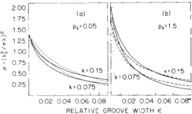
veloped by Dombre and Hakim [101, and they (1) For systems with small k, we can calculate correspond, loosely speaking, to the large surface the properties of a particular continuous branch of tension limit, On the other hand, while most cx- steady state solutions describing cellular profiles perimentally observed solidification cells typically with deep narrow grooves. The Péclet number do have narrow grooves, at the same time they dependence of these solutions is weak, and for have small enough tip curvature that surface ten- p-~ 0 they reduce to the Saffman—Taylor-like

sion effects can be viewed as a small correction, solutions found earlier by Dombre and Hakim This seems to contradict the simple mapping [10]. The variation in wavelength of this branch is [12,10,29,31] onto the viscous fingering problem, parametrized in the matching theory by the rela-which associates narrow grooves with large surface tive groove width c near the tip, or, more conveni-tension effects. Therefore, even in the small Péclet ent to experiment, by the dimensionless LCS number limit, we believe that experimental fingers parameter ~ giving the tip position (see sections 9 may well belong to a different branch, and one to and 10, and fig. 13).

which the formal analogy to the viscous fingering (2) A fundamental assumption self-consistently problem does not apply. This will be discussed in satisfied by these solutions is the existence of a

detail in section 10. single matching region controlled by the small

It is interesting to note that a similar situation parameter c where deep narrow grooves can be has been argued to occur for dendritic growth in a matched to a particular class of finite amplitude channel [321. which may be viewed as the limit of cellular solutions describing the fingertip region. vanishing temperature gradient in DS. Here, two These finite amplitude solutions have wavelength branches of steady state solutions are believed to lying outside the planar instability band and evolve exist [33], a Saffman—Taylor like branch and a from the (infinitesimal amplitude) neutrally stable

250 J.D. Weeks et al.

/

Stability and shapes ofcellular profiles in directional solidification

planar instability band (i.e. the left hand solid makes systematic many of the earlier approaches curve in fig. 3). These solutions have a regular used by material scientists [2,3], the mathematical expansion in powers of k. The fingerlike solutions techniques (asymptotic matching [30]) as well as with narrow grooves (small ) resulting from the the results and their implications do not appear to matching also have wavelengths lying outside the be widely known in this community. We will thus planar instability band and have values of ~ of attempt to give a pedagogical and rather detailed order unity (see sections 9 and 10). account of them here, which also will focus on (3) Most numerical studies, using the same their limitations. We also give some details about two-dimensional model we consider here, find preliminary steps involving the introduction of narrow-grooved fingerlike patterns, but with wave- dimensionless units and other notational matters, length lying inside the planar instability band, since different conventions adopted by various These solutions are found well above threshold authors have caused some confusion in the litera-and evolve from small amplitude cells with wave- ture. Readers who are familiar with the problem lengths lying inside the planar instability band, and who are only interested in the main results presumably related for small k to the cells studied and their implications can proceed directly to by Sivashinsky [16] and others. The latter bifur- sections 3, 6, 7.4, 9 and 10,

cate off from the center of the planar instability The plan of the paper is the following. In band (indicated by the square in fig.

3),

and do section 2, we review the equations for directional not have a regular k expansion. The contrast with solidification. We use a simple two-dimensional the matching solutions discussed in (1) is evident model, the one-sided (solutal) model [ii, which is

(see section 10). still realistic enough to compare to experiments,

(4) Most experimental patterns also have nar- and which has been extensively studied numeri-row grooves, but with wavelength lying inside the cally. In this model, convection in the liquid is planar instability band. In the few cases where ignored and the imposed temperature gradient is experimental data on the tip position is available, assumed to be unaffected by the latent heat re-small values of~ are found, in qualitative agree- leased or by changes in the interface shape. These

ment with the LCS stability criterion ~ 0. This often are rather accurate approximations. We

gen-implies that the tips of experimentally selected erally ignore diffusion in the solid, taking the limit patterns have moved up substantially in the tern- where the diffusion constant ratio /3 DS/D tends perature gradient relative to the planar position to zero. Contrary to the conclusion the casual (see section 10 and fig. 13). reader might get from ref. [34], we argue that the

(5)

In contrast, the matching solutions for small one-sided model offers an accurate description of e have ~ of order unity, i.e. their tips remain close many features of interface patterns seen in realis-to the planar position. More detailed experimental tic systems with /3 small but non-zero. However, a measurements of ~ would be extremely useful to notable exception where the one-side model must determine the accuracy of the LCS ideas (see break down is in the reentrant part of the bubble

section 10). closure in fig. lb. This will be discussed in

ap-(6) The analysis of Brener et a]. [33] for crystal pendices B and C.

growth in a channel, as well as arguments by In section 3, we give a detailed discussion of Ungar and Brown [4], again suggest the existence the LCS stability criterion, together with its limi-of a branch limi-of steady state solutions in DS other tations. In section 4, we discuss the various dimen-than the ST branch. The analytic mapping of the sional parameters that characterize a DS

J. D. Weeks et al.

/

Stability and shapes of cellular profiles in directional solidification 251 scaling helps us assess the relative importance of a multiple-valued or reentrant interface where this the curvature corrections in the Gibbs—Thomson approximation must break down.

boundary condition at the tips of real experimen- Most systems with small /3 also have relatively tal patterns and hence the accuracy of the LCS small values of the partition coefficient k, since condition. In section 5, we derive exact equations impurities that do not diffuse well in the solid expressing flux conservation which serve as a use- tend to be rejected on solidification, Thus the ful starting point to yield approximations for the limit of small /3 and k analyzed here is relevant to tail (section 6) and for the tip (section 7). After a many experiments. The main exception concerns discussion of the behavior of the resulting finite liquid crystals, where both /3 and k are of order amplitude cellular solution in section 7, we then unity [19]. Here the deep grooved patterns of turn in section 8 to the asymptotic matching anal- primary interest to us in this paper are usually not ysis which yields approximate shape expressions found,

for cells with deep grooves. The results of this At the interface we assume local thermody-analysis are presented in section 9, while in section namic equilibrium as given by the Gibbs—Thom-10 we discuss in detail the implications of our son equation, so that the temperature at an inter-results and how they compare to experiments and face with impurity concentration c, and curvature

other theoretical work. ic (taken positive when the solid bulges into the

liquid) is

T~(c,K) = TL(c,)(l -dK) (2.2)

2. Equations for the one-sided model

_ TM —mLc, — TMd,c. (2.3)

We consider the typical experimental setup Here TL(c/) is the (liquidus) temperature for a where a thin ampoule initially filled with a binary planar interface with impurity concentration c as melt with impurity concentration c~ is pulled given by the phase diagram. (The subscript i will through a temperature gradient established by in general denote a quantity evaluated at the inter-fixed hot and cold contacts. The gradient is large face; we use a superscript s to denote the solid enough that solidification must occur as the melt phase.) In (2.3) we have assumed a simple linear is pulled from the hot to the cold region of the phase diagram as in fig. 4a, appropriate for dilute cell. The impurity concentration c in the melt solutions, and expanded about the pure solvent at obeys the diffusion equation

=

D

V2c, (2.1) ~ z~

where c tends to c~ far in front of the interface. T1

--In principle, there is a similar equation in the solid 0 ME involving Ds, the diffusion constant in the solid. L~ LT

However, for most metallic or plastic crystal solid- 0 0 uo~l

ification systems the diffusion constant ratio /3 C

D~/D is of order of or smaller than 102, and in

many expressions it is a good approximation to Is) )b)

ignore diffusion in the solid entirely, thus arriving Fig. 4. (a) Phase diagram illustrating the varioustemperature at the one-sided model, with D~’ 0. The one-sided and concentration parameters defined in the text.(b) Phase model is much simpler to treat analytically, and diagram in terms of the dimensionless concentralion variable we find that il offers an accurate description of u. Along the vertical axis,the temperature has been eliminated in favor of the height variable z with the aid of (2.6). The

many features of interface patterns seen in realis- . . . . .

position ~= is the point where T= in (a). and z= 0

tic systems with /3 small but non-zero.

In

ap- denotes the steady state planar interface position wherec~=

252 J. D. Weeks ci al./ Stability and shapes of cellular profiles in directional solidification

(a) (b) in d(0) is much larger. However, unlike what is

MELT believed to be the case for free dendritic growth

~ [37],

anisotropy is not an essential feature for the

existence of steady state patterns in DS. Thus, for -dz - ds

notational simplicity in the equations that follow,

~fl

we consider the case a4will also report some results of calculations with= 0 or

cI= ci~,

although we

a4

nonzero.

A second boundary condition expresses local

0 X

conservation of impurities:

Fig.5.Illustration of our coordinate conventions.

=

—D(A

.vc),. (2.5)

Here fr~is the normal component of the interface

TM

to first order in

c and ic, with [36] mL velocity, ~c, c~— c~the “impurity surplus”

re-dT1/dcj. jected into the liquid as the interface advances,

Strictly speaking, if crystal growth is to occur, and (ñ Vc)4 the normal component of the con-there must be some kinetic undercooling [1], but centration gradient at the interface, Eq. (2.5) this is usually very small for growth in the cellular equates the rate at which impurities are rejected at regime. The local equilibrium assumption (2.3) the interface to the diffusion flux into the liquid. generally produces little quantitative error and is Again we have assumed that the one-sided model standard for the theoretical model studied herein, is accurate, and ignored any diffusion flux into the See, however, section 10 for some remarks about solid.

the possible importance of interface kinetics in We assume that the contacts set up a linear

certain limiting cases. temperature gradient, thus neglecting the generally

Surface tension corrections show up in the term small corrections due to latent heat generated at clic in (2.3). For cubic crystals, we assume the the interface. Then the temperature field in a specific form y(O)= ‘i’0(l + a4 cos 40) for the an- frame where the contacts are at rest is simply

gular dependent surface free energy, but our

re-T=1~+Gz, (2.6)

sults can easily be generalized to arbitrary ‘y(O).

Here 0 is the angle between the interface normal where 7~is a reference temperature (chosen later

and the z axis, which is taken along the pulling to equal that of the steady state planar interface) direction, See fig. 5. The quantity d(0) appearing and G the imposed temperature gradient. Evaluat-in (2.2)

and (2.3) is proportional to y

+d2y/d02. ing (2.6) in the liquid at the interface and

combin-and can be written [37] ing with (2.3) gives an equation describing the

= c10(l — a4 cos

40).

(2.4) variation of the impurity concentration as a

func-tion of interface posifunc-tion and curvature,

Here

d0 y1~/L is the intrinsic capillary length,

with L

the latent heat per unit volume and a4

= c~= c0 —

(G/m1)z,

— (~)TM/mL)K, (2.7)

15i~4for the specific form of ‘y(O) assumed above, where c0 is the liquidus concentration at

tempera-In most materials d0

is of the order of atomic ture 7~.In the same way, we can derive an equa-dimensions, and hence much smaller than the tion for the concentration c;”

in the solid at the

radius of curvature of typical interface patterns, interface, Using (2.7),

the result can be written

Nevertheless, the curvature correction in (2.3) will

c~=kc,,

(2.8)

turn out to play an important role in establishing

the overall scale of patterns found in a DS experi- where, for the simple linear phase diagram of fig. ment. Although the anisotropy a4 in the surface 4,

the

partition coefficient k is a constant,

tension is generally rather small (of the order of a

J. D. Weekscial. / Stability and shapes ofcellular profiles in directional solidification 253 Graphically, k is the ratio of the liquidus to the Here

solidus slopes.

We are interested in steady state solutions of u, —u~= u,— k(u, —

I)

(2.17a)

(2.1), (2.5) and (2.7) and note that the patterns are = 1 — (i — k)(z,/l~1-— d1K), (2.17b)

stationary in a frame where the contacts are at

rest, i.e., a frame moving at velocity V in the +~ is the dimensionless “impurity surplus” and we direction with respect to matter in the sample. We have used (2.12), (2.13) and (2.15) to arrive at use this moving frame in all that follows. For such (2.17b). Eq. (2.15) follows directly from (2.7) and stationary patterns V~= Vcos 0 (see fig. 5), and introduces two fundamental lengths [38]: the

ther-the left-hand side of (2.1) evaluated in ther-the moving mal length.

frame becomes — V ac/az.

m1~c0/G, (2.18)

The simplest solution of the steady state

equa-tions describes a planar interface, for which the and the chemical capillary length, concentration field satisfies

dO~d~TM/mL~c~. (2.19)

c= (c0— c~)e ~ + c~. (2.10)

Here we have chosen

z= 0 as the location of the The chemical capillary length d0 is normally

planar interface, where by definition c- = c~1

and

much larger than

d0.

From (2.15) and

(2.13) we

=

J~,

and defined the diffusion length see that the temperature T~ at z= l~-is such that

the liquidus concentration equals cc~,while from

‘I) D/V. (2.11) (2.12) the temperature 7~and the location z= 0 is

To determine c0 in terms of experimental parame- fixed by the requirement that the solidus

con-ters, we use eq. (2.5) and find centration equals c,~.

See fig. 4a, Note from (2.15)

= icc0 = ~. (2.12) that the equation for the liquidus line in the

modified phase diagram in fig. 4b is Thus the planar interface is located at that point

in the cell where the impurity concentration incor- uL(z) = 1— z/l~-. (2.20)

porated into the solid,

kc~,

equals the limiting Since the curvature ,c1 is greater than zero at the impurity concentration c~. This global

conserva-tion condiconserva-tion is required for steady state planar tip of a solidification pattern, and we expect no

growth. See fig. 4 “concentration deficits” with u <0 in front of a

We use the planar solution to help define a steady state pattern, eq. (2.15) shows that the tip dimensionless concentration field, u, scaled so that position_{In the next section we discuss the LCS stability}z1 of any such pattern is such thatz~<l-~.

typical variations are of order unity:

criterion that sets an approximate hound on the

u (c— c~)/~c0, (2.13) position z1 of many experimental patterns.

where, using (2.12), 4~1c() c0 — c~= c0 — ~. When diffusion in the solid can be ignored, we

Clearly U1)=

I and

u~= 0 from (2.12), and in can relate the concentration field in the solid to

general u= 0 far in front of the interface. See fig. that “frozen in” at the interface above. In the

4h, where the phase diagram is replotted in terms steady state. eqs. (2.8) and (2.13) then imply of the variable u and the position z in the cell, us( x, z) = k [u( x, z, (x)) —

II,

(2.21)

using (2.6).

Eqs. (2.1), (2.3) and (2.5) in the steady state can where u(x, z(x)) = u gives the concentration in

then he put into the reduced form [1,261 the melt at interface position z1(x). As a result,

i au we need explicitly consider only the field u in the

vu + = 0, (2.14) liquid and at the interface, as in eqs. (2.14)—(2.16).

Ii)

a~

u,= I — :,/l-~— d~,c. (2.15) Clearly, however (2.21) must break down if we

254 J.D. Weeksc/al./ Stability and shapes oJ cellular profiles in directional solidification

of z,(x). This is discussed in appendices B and C, where we define a basic dimensionless control but for now we will assume the patterns are such parameter v:

that there exists a single-values interface for which

the one-sided model with Ds = 0 remains accu- ~ = Vm1&0/GD.

(3.2)

rate, _{Note that v is directly proportional to the velocity}

V. The usual CS criterion for instability of the

plane follows from (3.1) where we note that global

3. Interface stability and constitutional supercool-

conservation requirements force the plane to be

ing

located at z, = 0, where Zlu,= 1. (See fig. 4b or eq.

(2.17b) and the discussion after eq.

(2.12).) Thus.

The first successful stability criterion for a as V is increased the planar interface at z = 0 is

planar interface in DS was based on the idea of predicted to be stable until a critical value of V is constitutional supercooling [1—3]. As suggested in reached such that

the introduction, we can argue as follows. The _(.5

phase diagram (see fig. 4a) applies to stationary ‘i = 1. (3.3)

planar interfaces and delineates the two phase

region between the liquidus and solidus curves This criterion is surprisingly accurate, given the where a stable (one-phase) liquid at a particular T simplicity of the CS argument. For materials with and c cannot exist. The basic idea of constitu- small k, the fundamental linear stability analysis tional supercooling (CS) is [1—3] that in the steady [11 predicts only small changes in the critical value state we can assume local equilibrium and apply of v. i.e., i’~ I. At the very least, the CS theory

these same thermodynamic concepts to the moving provides a very useful “rule of thumb” for esti-planar interface and to the melt just in front of the mating planar interface stability [1].

interface. This idea was implicit in rewriting the However, the arguments leading to (3.1) seem phase diagram as a function of z in fig. 4h. nearly as plausible as before when applied locally In general, we assume local thermodynamic to the melt in front of the tip of many (non-planar) equilibrium at the interface by using the Gibbs— patterns, provided that the curvature corrections Thomson boundary condition (2.15). Constitu- in (2.15) are small. In particular, we need to use tional supercooling makes the very plausible asser- only the boundary conditions (2.15) and (2.16) and tion that the moving planar interface remains sta- the local symmetry in the tip region (nearly planar, ble as long as the melt just in front of the interface with 0~= 0) to arrive at (3.1) with ~u, = ~u1, the

also satisfies the thermodynamic requirement for impurity surplus at the tip. When curvature cor-single phase stability: the concentration there rections to ~u1 in (2.17b) are small, eq. (3.1) can should not fall into the two phase region of the he reexpressed as

phase diagram. (v—i)— (1 — k)z~/li4~ 0. (3.4)

Since the concentration at the interface is on

the liquidus line from (2.15), the CS condition for Eq. (3.4) predicts that the tip position z~of stability of the liquid just in front of the interface stable patterns with v> I must move up in the reduces to the following requirement. The (dy- cell, relative to the planar position at z= 0, until

namical) gradient jdu/dz = L\u,//r) determined the smaller impurity surplus ~u1 allows (3.1) or

from the boundary condition (2.16) must not cx-

(3.4)

to hold true. It is natural to conjecture that ceed the liquidus slope Idu /dz

I

= I//T given in the operating point in real experiments should be

fig. 4b or eq. (2.20), where the temperature depen- close to the one that requires the least forward dence of the phase diagram in fig. 4a is reex- motion, i.e., the region where ~‘ 0. We refer to pressed as a function of position z in the cell, This this condition as the LCS criterion.

criterion can be reexpressed as Note also that just as the Mullins--Sekerka

instability of the plane is a finite wavenumber

J. D. Weeks et al./Stability and shapes of cellular profiles in directional solidification 255 cells predicted by LCS for ~ 0 actually corre- As we will see in the rest of this paper, the

sponds to a finite wavenumber instability [39].

condition ~ 0 will

also have important

implica-This is indeed confirmed by a more careful analy-

tions for the validity of various matching theories

sis [21], which also shows that the LCS criterion for DS. To analyze these questions in more detail,

= 0 gives an upper bound

to the distance

z that we first

discuss in the next section a choice of

the tips of patterns have to move up to regain

length scale in the theory that renders eqs. (2.14)—

stability. For a periodic array of cells with

~ 0, (2.16) dimensionless. Our choice will be particu-we envision that the instability in practice corre- larly useful in helping to determine the relative sponds to a mode in which some of the cells move importance of the curvature terms in (2.15)

and

up slightly, while others stay behind and subse- hence the applicability of the LCS criterion. quently get pinched off.

Ref. [21] also shows that curvature corrections neglected in

LCS

become more important at larger

v. Indeed corrections to the LCS picture must

4. Experiments and theoretical parameters

surely be taken into account at large v> 1/k (usually in the dendritic regime), since (3.4)

com-bined with (2.15) would then predict z > 1T’ thus There

are many parameters that can be varied

implying an unphysical “concentration deficit” at in a directional solidification experiment. The the tip with ti <0. However, for small k

and

v

in

choice of the solvent and impurity system fixes the

the cellular regime, corrections to LCS appear to material parameters k,. I~,, d0, D

and

mL.

In

be small,

principle, one can still vary the limiting impurity

Of course, these arguments are only suggestive,

concentration in the melt

c~,

the temperature

The LCS condition (3.4) is not exact, even for the gradient G, and the pulling velocity V,

to produce

plane at z=

0. However, in that case we can

a

variety of patterns, whose properties can be

compare its predictions to those of an exact linear characterized in terms of the parameters 1iJ~

~-1-stability analysis. For materials with small parti- and d0 given in eqs. (2.14)—(2.16). We consider tion coefficient and small /3 = D.,/D it does give a here the usual experimental set up where c~ and

very accurate estimate. Similarly, we expect that G

are fixed and

V is increased above the threshold

the linear stability analysis of the fingertip region velocity

1~to produce instabilities in the planar

of many nonlinear patterns would agree rather interface.

well with the predictions of (3.4). We hope this In such an experiment, the choice of c~fixes c0 will be investigated in the future. Measurements of and the location z = 0 from

eqs. (2.11) and (2.12),

the tip temperature similar to those by Esaka and

as well as the chemical capillary length

d0

from

Kurz [40] yield all the necessary information to eq. (2.19). Choosing G then determines the ther-determine i’ (see section 10 for a more detailed mal length ‘T

from eq. (2.18). As

V is increased,

discussion of these experiments), the diffusion length I~= D/ V decreases at fixed

As shown in appendix D, one can define a d0

and

1T’ We are interested in properties of the

measure of constitutional supercooling for a gen- periodic cellular patterns that emerge, in particu-eral point near the interface of a fingerlike pat- lar their wavelength A and parameters that

char-tern, although the analogy to the

planar case is acterize their shape such as the tip position and

less compelling when 0, is non-zero. Using this, we the groove width,

can establish the general validity of the frequently We can choose one of the four lengths d0, 1T’

256 J. D. Weeks ci al./ Stability and shapesofcellular profiles in directional solidification

has already been mentioned in section 3, where we Except for the very flat part of the curve in fig.

3

defined

extremely near threshold, which we do not

con-sider henceforth, A

is essentially independent of

= Vm1~~c12/GD. (4.1) the value of the partition coefficient k (at least for

small k) and is accurately approximated by A,(k Since the constitutional supercooling instability

= 0) A~where [41]

criterion v~= I is usually very accurate, we can

think of v as the ratio of the pulling velocity V to PdOID 1/2

the threshold velocity fr~.The cellular regime of A1~=

2~(~j)

.

(4.3)

interest to us in this paper is found at larger v

with v— I of 0(1); at still larger pulling speeds (This result arises [1] when one considers a small

v ~ 10 a dendritic regime is usually found. We will interface perturbation of the form exp(iqx+ cat);

not consider the latter regime in this paper. by definition q.,

2~/A~

satisfies w(q~)= 0.) Thus

The resulting patterns are often characterized a scale related to A1~ seems appropriate. In the

by the Péclet number p, where following, we take the half wavelength A~/2as the

unit of length. Measured in these units, the

dimen-A

AV

= -~-~

(4.2)

sionless half wavelength a

(A/2)/(A~,/2)of the

experimental patterns of de Cheveigné et al. [8] is some small multiple of unity. We expect this result relates the scale of the pattern (the half

wave-to be true for most experiments, where we assume length) to /~. the typical range of the diffusion that the selected patterns have wavelengths falling

field in front of the tips. Experimental cells can

within the planar instability hand towards the have Péclet numbers as large as 0(1).

left-hand side. Note from (4.3) the well-known These ratios [38] arise naturally in the resulting

result that the experimental patterns are found on dimensionless equations when l~ is chosen as the

a length scale that is intermediate between the unit of length. Another common choice in

theoret-ical work is A itself. However both of these choices, (usually small) scale d0 set by surface tension forces and a macroscopic scale‘T or

while perfectly consistent and offering some

theo-Our basic equations (2.14)—(2.16), written with retical advantages, can cause some inconvenience A~/2 as unit of length, then have the dimension-when comparing theory and experiment. Thus the less form

choice I~-~gives a scale that is not obviously the size of a typical pattern.

(4.4) On the other hand, the choice A gives a length

scale that by definition is the size of a pattern. pjiu,) cos 0= —(h - vu),, (4.5)

However, conceptually this is somewhat

dissatisfy-p / v—I

ing since that scale is not fixed in advance: the ~ — — —~-~ ~, + —k

i,

(4.6)

prediction of A is actually a goal of the analysis. ‘— P ~

)

With this choice it becomes natural to report

where we have defined theoretical results in terms of a dimensionless

parameter a relating the surface tension to the ~ AY~/2/~~.

(4.7)

pattern wavelength. See eq. (9.1) below. Using

this, it is possible to extract the actual (dimen- in analogy to the usual Péclet number p. in eq.

sional) value of A. (4.2). In general we use the subscript s to denote

We make here another choice of length scale quantities associated with the stability length. It which avoids some of these problems. As il- should not he confused with the superscript s lustrated by fig.

3,

most experimental cellular pat- denoting the solid. Note that p= p~a.(To obtain

J. D. Weeks ci al./Stability and shapes ofcellular profiles in directional solidification 257 by p

and ~r2

a,, by a,

as defined in eq. (9.1)

pendent of

the position of the segment, since no

below.) net flux can escape through the vertical lines of

For simplicity in notation, we do not indicate symmetry. See fig. 5.

by a special symbol in eqs. (4.4)—(4.7) and those Using the notation of (4.4)—(4.6), a

dimension-that follow dimension-that the coordinates x and

z are now less measure of this integrated flux in the melt for

dimensionless, with At?,/2 as unit of length. The

z > z.

with

z~

the tip position of a pattern, is

presence of other dimensional (e.g.,

l~

and lr) or

a

~au\

(5.2)

dimensionless (e.g.,

p,,, v)

parameters in the equa-

F(z) =

f

dx( u

tions themselves will indicate the proper dimen-

0 ~

)‘

sions to assign to the coordinates, Note also that

where z

denotes the segment position,

a is, as

throughout this paper, A and A~will always de- before, the dimensionless half wavelength, and we

note the

dimensional wavelengths, whereas a

de-have noted that vu-

2=

au/az.

Far in front of

notes the

dimensionless

half wavelength of a

pat-the interface we know that

u=

au/az

= 0, so

con-tern.

servation of impurities in the steady state requires

Finally note that in experiments where the

that

F(z) = 0 everywhere. If we consider an

arbi-selected wavelengths fall inside the planar

instabil-ity band, we have a>

1, The curvature at the tip

trary

line segment whose vertical position z satis-fies z < z~we have similarly

of these patterns is very roughly given by a~.

(This estimate is exact for fingers of vanishing

au

groove width whose tips are semicircles.) The F(z) = 0=

(

dx(u +~~1~) “0 \

curvature correction term in (4.6) is thus

ap-a

proximately given by (v—1)p,,/(vir2a). In the +kf dx[u(x,

z,)—11,

(5.3)

cellular case we have ~i —

I of 0(1), and usually

p~~ 1, so curvature effects are numerically small

in (4.6), unless the tips have moved so high that

u

where we have used eq. (2.21) to rewrite the

im-is very near zero. purity concentration in the solid in terms of that

found at

the fluid interface directly above. Here

x x1(z)

and

z~ z,(x) give the interface

posi-tion as funcposi-tions of z and x, respectively.

Dif-5. Flux conseri’ation

ferentiating

(5.3) with respect to

z gives the exact result [26]

A study of the impurity flux provides a

power-ful means of analyzing eqs. (4.4)—(4.6). The (di- dx i —

(

au)

]

~

/

a ~

a2 ~

a

+f

dx(

mensional) impurity flux in the moving frame at

dz

[

z

-~-~-+p

any point in the fluid is given by

dx

J=

—Dvc— VcI, (5.1) k~(u,1)0. (5.4)

z

where the first term is the usual diffusion flux, and Eq. (5.4) is the basis for the tail analysis carried the second is the “convective” flux of impurities out in this paper. It is equivalent to eq. (4.5), as in our moving reference frame induced by the shown in appendix B, which also discusses the constant pulling velocity V

in the

—z

direction. In

more

general case

with /3

D5/D > 0. Our

the solid phase, by ass~umption D5=

0, so that

strategy

is to reexpress quantities involving the

only the second term remains, diffusion field in (5.4) in terms of quantities in-For a spatially periodic steady state pattern, it volving the interface shape. This generates an ap-is clear that the impurity flux in the —z

direction

proximate differential equation for the interface

258 J. D. Weeks ci al./ Stability and shapes of cellular profiles in directional solidification

6. Tail approximation

(3.4) gives the LCS stability criterion. (Note that

in (3.4), z~was written in dimensional units.) For

Eq. (5.4) has terms involving the interface shape

our purposes here, ~ gives information about the

x,(z). This is

a convenient representation for the

width of the planar two phase region

L~u1(z),

and

interface shape deep in a groove since here the

can also be thought of as a dimensionless measure

slope dx1/dz =

cot

0 (see fig. 5) is small, Using of vertical distance. As we will see, ~‘

appears

this fact and the narrowness of the groove will

repeatedly in the rest of this paper; this is why the

allow us to approximate eq. (5.4) for deep grooves,

ideas of [CS turn out to be of relevance to the

The method is very general and can be improved

matching theories. The tail equation (6.4) has also

systematically. However, we expect the lowest

been derived independently by Mashaal et al. [29]

order results given here to be sufficiently accurate All the approximations leading to (6.4) can be

to describe the groove region seen in many experi- improved systematically, but the lowest order

re-ments,

suit will prove sufficiently accurate for our

pur-The terms involving u,

in

(5.4) can immediately poses here. Deep in the grooves, terms involving be reexpressed in terms of the interface shape the curvature become negligibly small and (6.4) using the Gibbs—Thomson equation (4.6). More- reduces to

over, terms involving field derivatives like

(au/az),

can also be approximated accurately by differenti- ~‘

dx,/dz

=p,,x,,

(6.6)

ating (4.8) since which has the solution

PSi 2

u,(z) u(x,(z), z) = I — _PcIz + ~ (v—

I)KJ,

x,(z) = ~

(6.7)

(6.1)

with A0 an integration constant.

so that, by the chain rule, Thus as —~~ (i.e., z —~ —

~),

grooves are

predicted to close as a power law x, z

du,

/

au

\ /

au

\ 1 dx, where the exponent t=

1/(I

— k)

depends only

-~ =

~

+ (6.2) on k and is near unity for small k. This limiting

result has been known for some time now, and is

= — ~ — v—

1 dK).

(6.3)

usually attributed to Scheil and Hunt [2,27,28].

P~

For a real physical system with /3

D5/D small

For small dx1/dz we have from (6.2) that but non-zero, (6.7) must eventually become

mac-(au/az),

du1/dz, and similarly, using also the curate sufficiently deep in the grooves because of narrowness of the grooves,

(a2u/az2)

d2u1/dz2. the effects of diffusion in the solid ignored in the

Finally, for narrow

grooves we can approximate one-sided model. (Of course, our assumption of a the terms under the integral in (5.4) by their linear phase diagram as in fig. 4 must also become values at the interface. In this way we find from inaccurate, e.g., at a eutectic point, but we do not (5.4) our basic groove equation [26] analyze this possibility here.) In appendices B and

dx, / 2

dK

C we discuss how

the results of this section are

d

—

(I

—k)p,,~r2(v

1)tc

— rr (v—

1)

I

modified when

/3

is

small but non-zero and derive

dz;

an upper bound to the breakdown distance ~Th

d2K dK beyond which (6.7) cannot be trusted. We also

— x,~2(

~

—

1)

— ~ ~- 2( P—

1)

~ make some more general’ remarks about both the

dz

(6.4) utility and the limitations of the predictions of the one-sided model,

Here Eq. (6.4) is much more general than the limiting

Scheil result (6.7). The terms involving the

curva-~=(v-I)—(1-k)p,,z (6.5)

J.D. Weeks et al./Stability and shapes of cellular profiles in directional solidification 259

vertical Scheil shapes must somehow “bend over”

finite amplitude solutions (i.e., solutions without

smoothly and join to tips with larger curvature,

deep grooves) for which the diffusion field is

They also play a role near the closure region of nearly one dimensional, i.e., u u(z) only, even

finite depth grooves,

though the interface shape is far from planar. We

Eq. (6.4) is a nonlinear fourth order differential can provide a simple treatment of such solutions. equation for the interface shape x1(z), as is easily In the following, zm

represents the minimum value

seen by writing the curvature as ofz~for these solutions.

K= _(d2x,/dz2)[I +

(dx,/dz)2]

-3/2

(6.8)

7.1. The k —O~ limit

It can be easily seen by direct substitution that After requiring that all solutions reduce to (6.7) in the limit k—f 0~,the one-dimensional field

deep in the grooves as

—*

oc, there are still two

integration constants left free to vary [42]. Rca-

u(x. z) = uB(z) = B0 e~’~

(7.1)

sonable choices for these constants produce solu-

provides an

exact

solution both for the diffusion

tions that indeed bend over and resemble the

_equation

(4.4) and the

conservation condition (4.5),

beginnings of a cell tip [43]. It would be interest-

independent of the shape of the interface [44].

ing to compare the solutions of (6.4) to experimen-

Given this asymptotic solution to the diffusion

tal groove shapes, since we typically find that the

field, one can then integrate the Gibbs—Thomson

limiting Scheil shapes are accurate only for rather

equation (4.6) in the form

larger.

P5 2(p1)K]

(7.2)

In order to determine the integration constants B0 e” =

1

— — [z, + rr

P

explicitly, it is necessary to examine the region

to derive a variety of interface shapes consistent closer to the finger tip where the approximations

_{with this field and hence with all the DS steady}

leading to

(6.7) become inaccurate. This occurs

state equations. Our goal is to explore this

particu-because the width of the groove increases and the

lar class of tip solutions for which u(x. z)

reduces

slope dx1/dz becomes very large.

to (7.1) in the limit

k—~0~.To do so, we will first

This cell tip region is the subject of the

follow-analyze the finite amplitude

k—s0+

patterns given

ing sections 7 and 8. Once

an accurate description

of the tip region has been found, we still have the

by eq. (7.2) and then discuss how these solutions

are modified for k

small but finite. The use of

problem of combining the tip and tail

approxima-these solutions to construct the tip shape of cells

tions to obtain a globally acceptable solution. As

with deep grooves is discussed in the next section.

shown in section 8, for a class of solutions with

Although the one-dimensional field satisfies

narrow grooves this can be carried out

systemati-both eq. (4.4) and eq. (4.5) in the limit

k—~0e, in

cally by using the asymptotic matching procedure

order that the solutions of (7.2) connect smoothly

introduced by Dombre and Hakim [10].

with those at small but finite

k

we need to impose

an additional global conservation condition. The

requirement that the total amount of impurities

7. Finite amplitude solutions and tip approxima-

left behind in the solid is the same as the amount

tions

entering through the liquid implies for the

one-sided model that all single-value interface shapes

The derivation of our tail equation (6.4) was obey a

simple and exact condition that is easily

rather general, exploiting only the steepness and

derived from the general flux equation (5.3).

narrowness of the groove, and holds for all values

Evaluating (5.3)

in the solid for z <zm and using

of the partition coefficient

k.

However, in order to

(4.6), we have for any

k>

0 (thus including the

find an equation that holds in the tip region, we

limit

k—~

0~)

will further assume that k

is small, which is the

a

usual experimental limit. Small

k

produces an

J

z,(x) dx = —172(v —

I)J

i(x) dx. (7.3)

260 J. D.Weeks et al./Stability and shapes oJ cellular profiles in directionalsolidifiCation

finite

amplitude

cells

of first order equations parameterized by the

arc-length s:

~

dz

~

+~-~H-~-

= -sin 0,

(7.6)

~J

•/_J

~ ~/

_dx

= —cos 0,

(7.7)

dO ~2 (IBoeTh:)zi), (7.8)

=

~“T

(,

~,,

dA

= —z, cos 0. (7.9)

~

~

~ ___~c-~~

____________________________________________

Eqs. (7.6) and (7.7) express exact geometric

prop-2 4 ~ erties of a curve (see fig. 5) and (7.8) reexpresses

X the original equation

(7.2). Finally,

A in (7.9) is

Fig. 6. Examples of finite amplitude solutions forp,,=0.15 and

(7.5b) evaluated at an arbitrary upper limit

s. =1.5. The horizontal lines indicate the location of the plane

It is most convenient to think of solving these

z=0.

equations by an iterative process. First pick an

initial guess for B0. For fixed B0, we can solve (7.6)—(7.9) as a simple initial value problem,

start-ing at the minimum and integratstart-ing upward. By

The latter integral can be evaluated exactly:

definition, the initial conditions are

Xm= 0, Om = 0

and

A,,=

0 at the minimum, but we can pick any

s~

dO

dx _~_ . 0. We then integrate [46] forward to the tip

K(x)dx=f —-_--ds=_f (sin0)ds

ds ds ds (maximum) of the solution where again0~= 0, and = sin°m—sin 0. (74) immediately find z, K and x1 a.

For fixed

B>>,

if

z~ becomes too negative the solutions do not

where we note from fig.

5

that dx/ds

= —cos 0. remainsingle-valued,

and we reject them.

Further-Here

s is

the arc-length and we have used the

more, even the single-valued solutions will in

gen-eral not satisfy the equal area rule

(7.5).

Hence

B0

fundamental

definition

K =

dO/ds.

For the

single-values cellular solutions like those in fig. Ia,

0,,, = 0~= 0, and (7.3)

reduces to

[45]

finite

amplitude

cells

fz(x)d

0

x=f’z,(s)~ds=0~

_ds

(7.5a)

~---~

r~

U

or

A(s1)

—f

z~(s)cos 0 ds=0. (7.5b)

We will refer to this condition as

the equal area

rule,

since it shows that for finite amplitude cells

-the areas above and below -the line z = 0 are equal.

See figs. 6 and

7 for examples. Note that with the

~

,~

sign conventions of fig. 5, 5~~>s1 in (7.5). x

It is useful both conceptually and for practical Fig. 7. Examples of finite amplitude solutions for i~= 4and